
Increasing the Utilization of Existing Infrastructures by Using the Newly Introduced Boundary Voltage Limits


Abstract
:1. Introduction
2. Legal Voltage Limits and Conventional Modeling
2.1. Voltage Limits Specified by Grid Codes
2.2. Conventional Grid Modeling
- PV node-element: The element’s active power contribution and the voltage magnitude at its boundary node are specified for the regarded instant of time. Additional Q-limits may be defined. Typical examples include producers, such as generators of conventional power plants, and reactive power devices, such as static var compensators and synchronous condensers.
- PQ node-element: The element’s active and reactive power contributions are specified for the regarded instant of time, either independent of the voltage at the boundary node or as a function of it. Typical examples include producers such as PV systems, storages, and neighboring grid parts.
- Slack node-element: The voltage magnitude and angle at its boundary node are specified for the regarded instant of time. The superordinate grid is usually selected as the sole slack node-element in the LF analysis at the MV, LV, and CP levels. Meanwhile, the largest generator may be defined as the slack node-element at the HV level, or the slack node-element may be divided between different large generators.
2.3. Problem Statement
3. Materials and Methods
3.1. Methodology
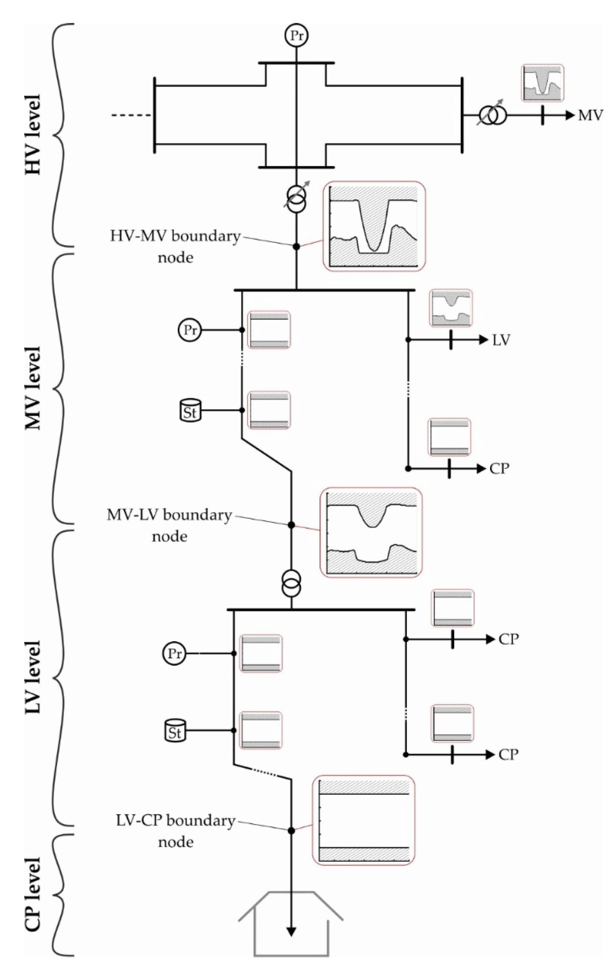
3.2. Structure of the Vertical Link Chain
 ,
,  , and
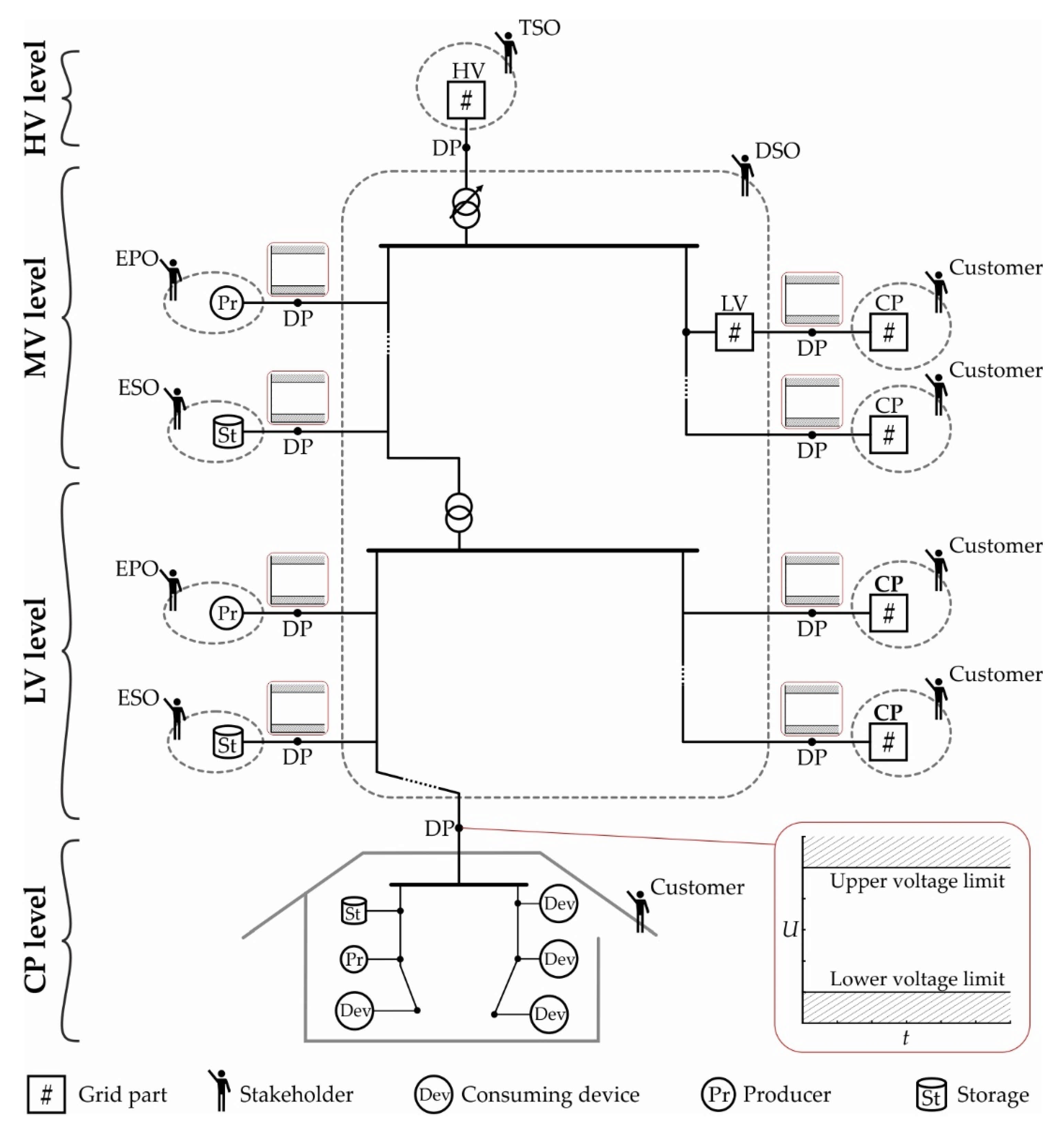
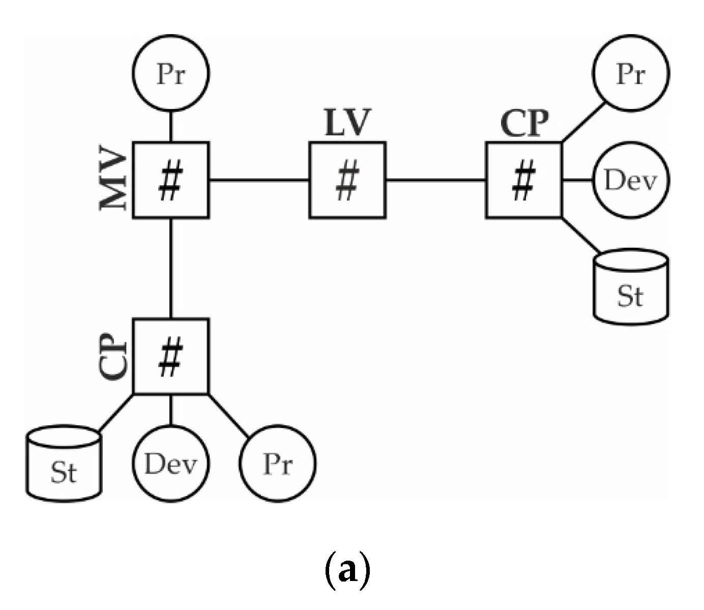
, and  symbols, respectively, and are connected to the Link-Grids through Boundary Link Nodes (BLiN), Boundary Producer Nodes (BPN), and Boundary Storage Nodes (BSN). Producer- and Storage-Links include the PV-system, generator, battery, etc., the primary control, and the interface to the corresponding SC. Both MV and LV grids are usually operated with radial structures. The CPs also include radial grids, i.e., the underpinned wires that interconnect the producers, storages, and consuming devices through the sockets and switches in the house. LINK-Solution intends the DSO to operate the STR, so the STR is included in the MV_Link-Grid.
3.3. Description of Simulated Grids
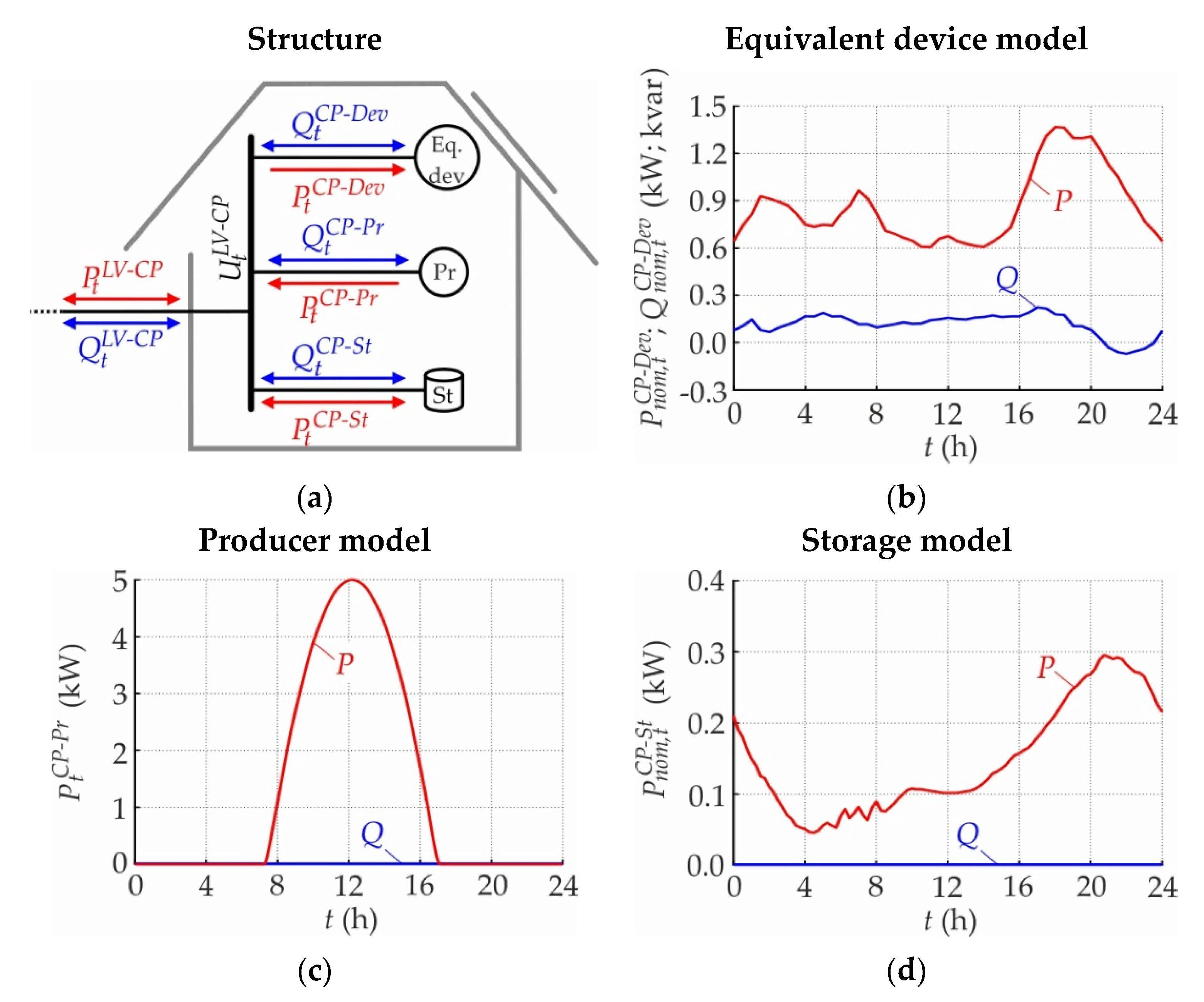
3.3.1. Rural Residential CP
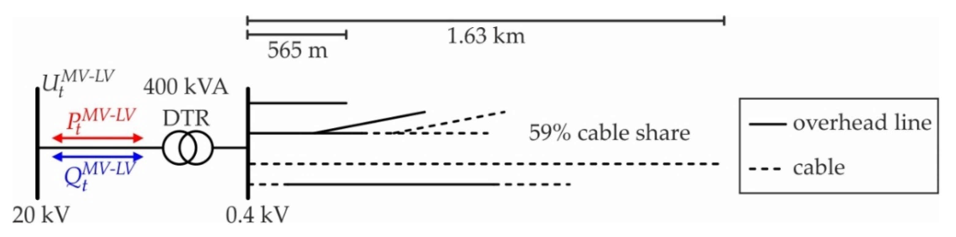
3.3.2. Rural LV Grid
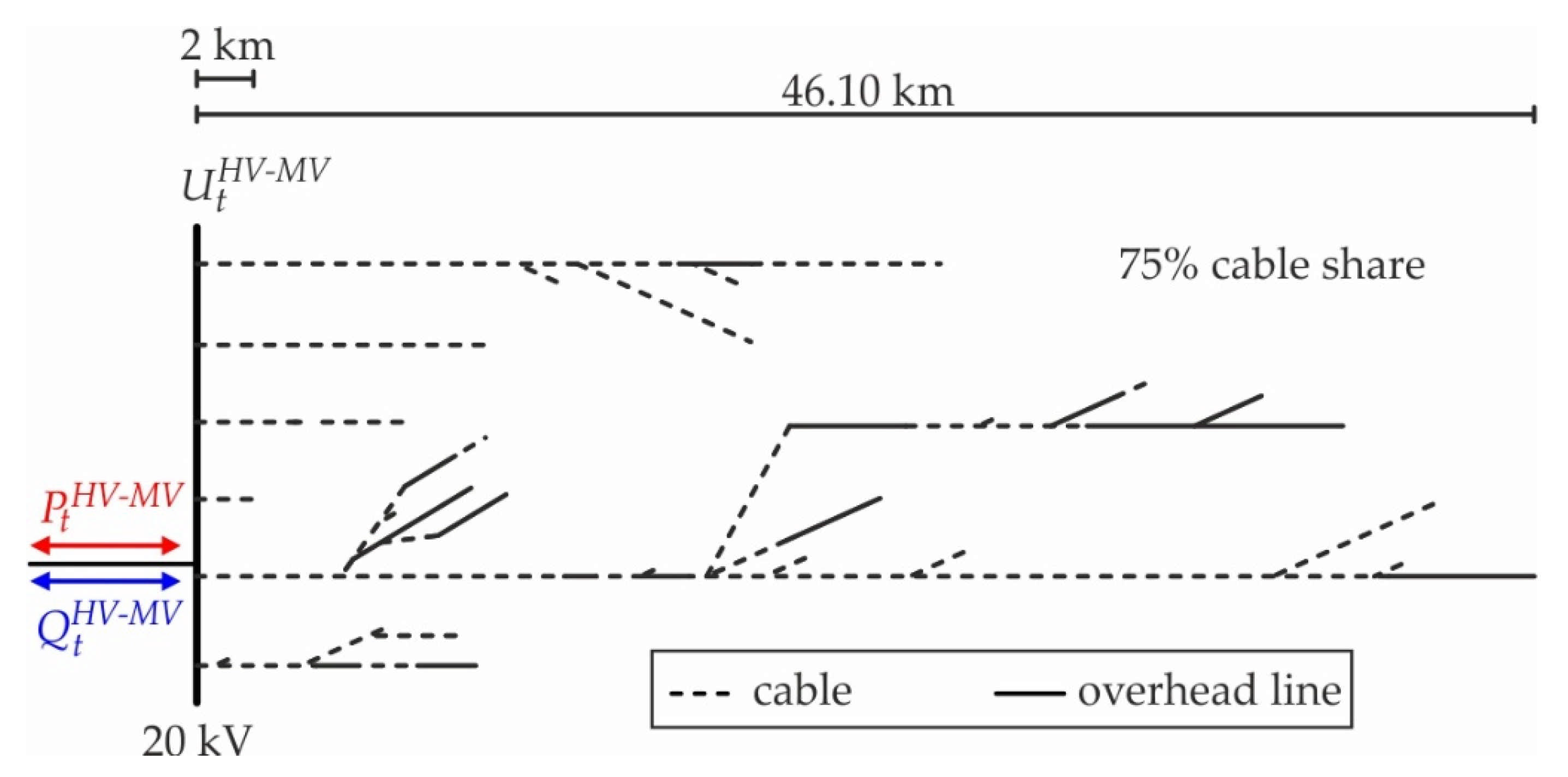
3.3.3. MV Grid
3.4. Calculation Procedure
4. Results: Emergence of Boundary Voltage Limits
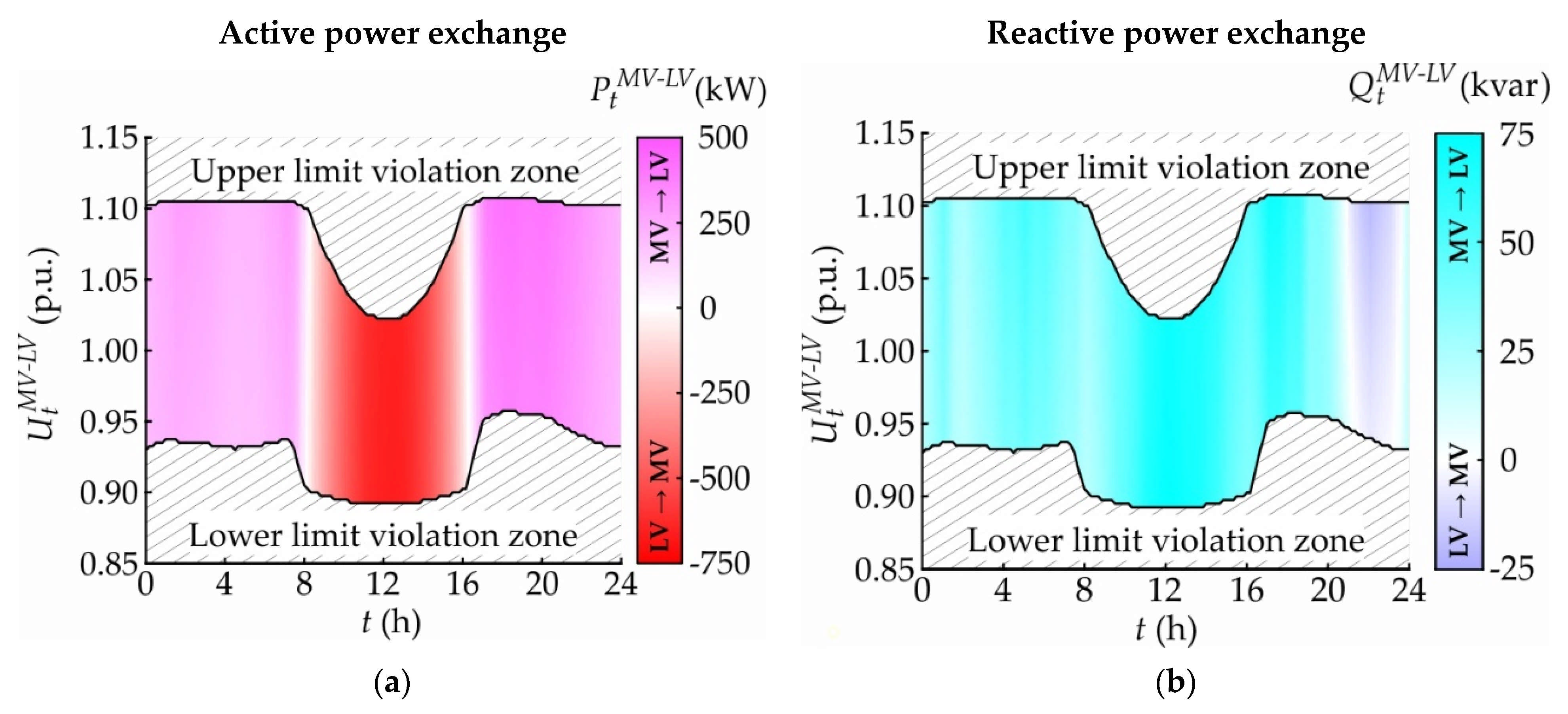
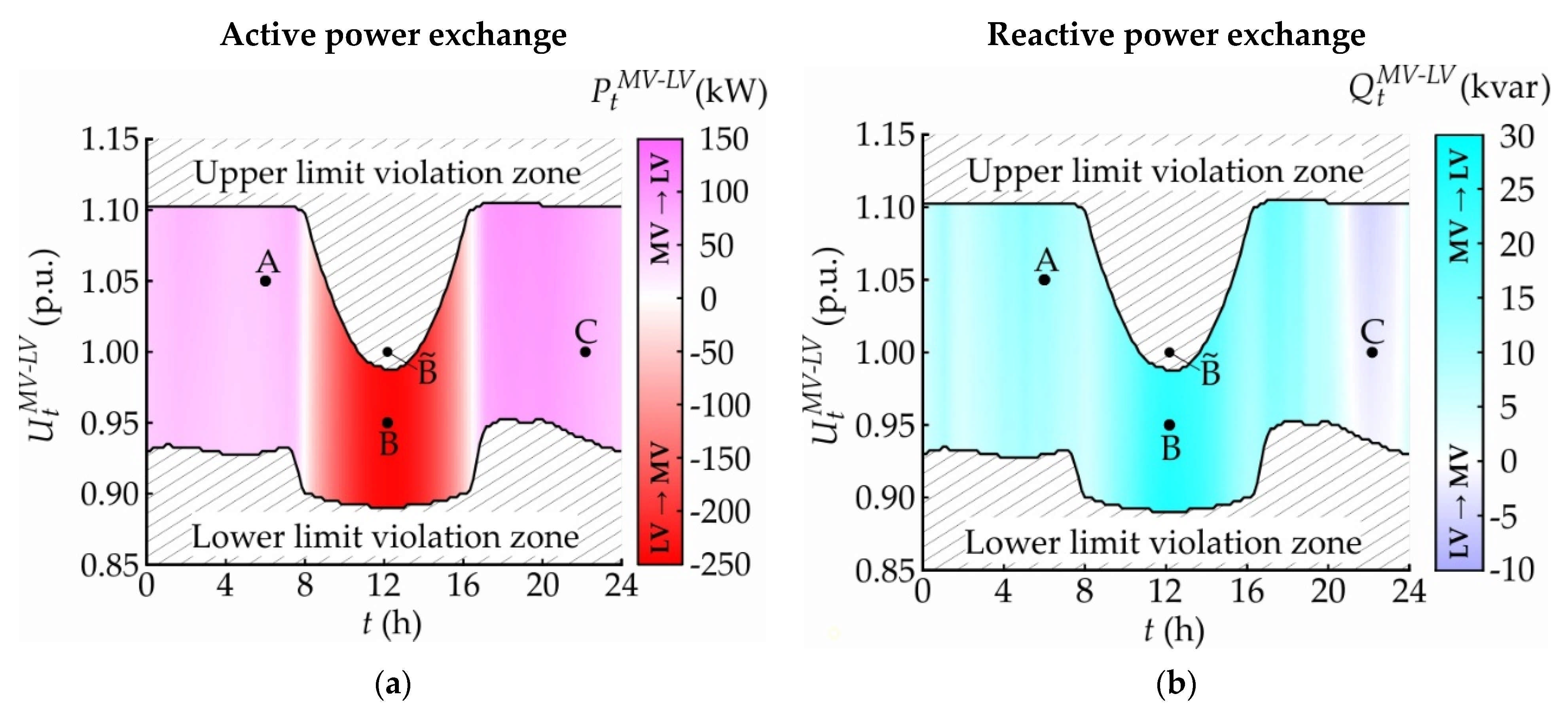
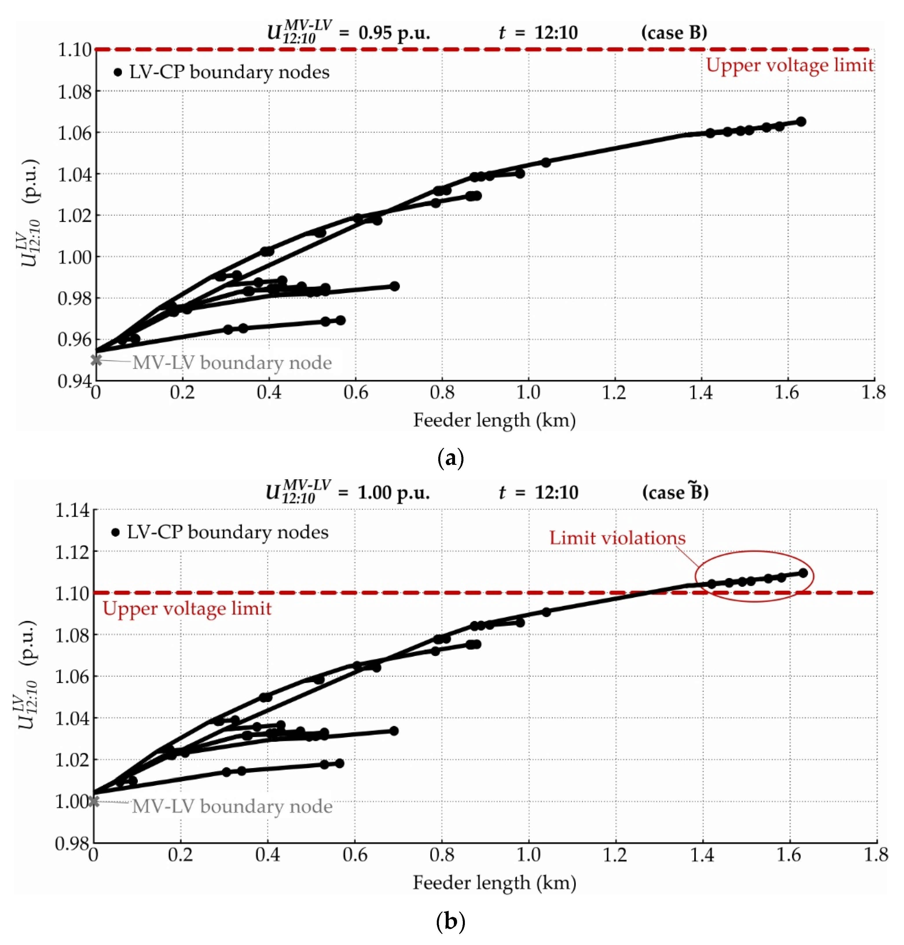
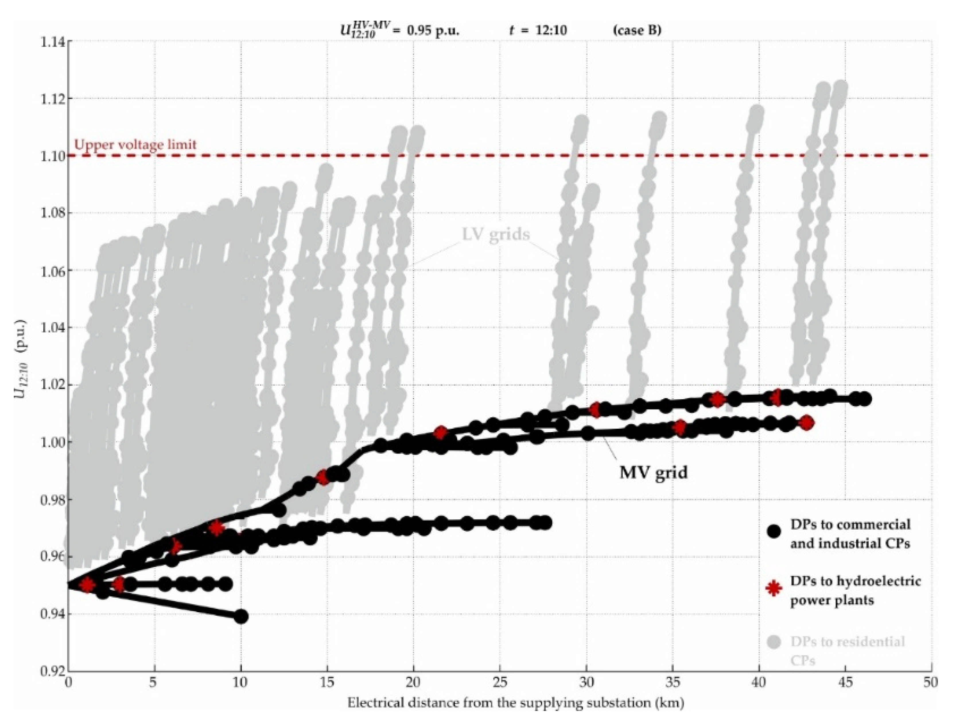
4.1. Voltage Limits Behavior on the MV-LV Boundaries
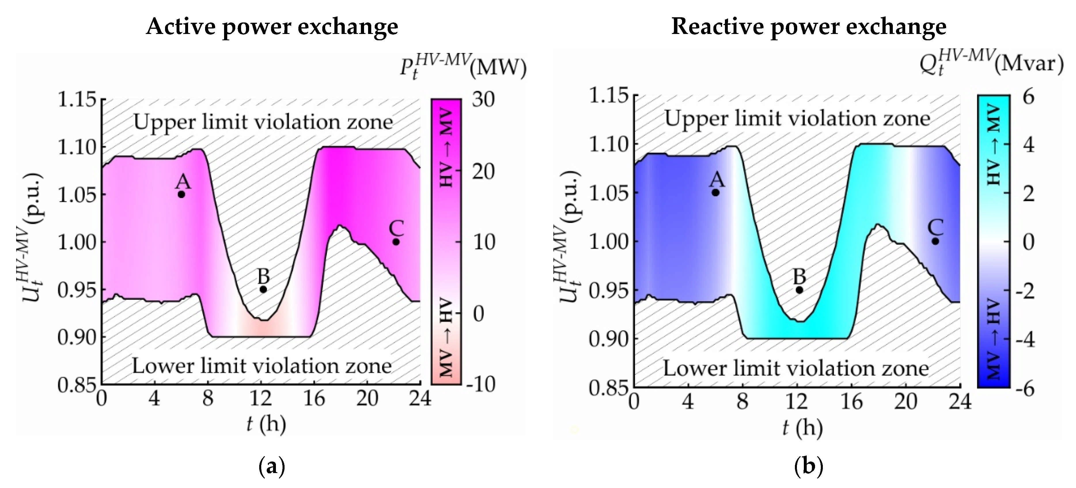
4.2. Voltage Limits Behavior on the HV–MV Boundaries
4.3. Deformation of Boundary Voltage Limits
5. Discussion
5.1. LINK-Based Grid Modeling
5.1.1. Overview of Lumped Link-Grid Model Parameters
- Upper Boundary Voltage Limit ();
- Lower Boundary Voltage Limit ().
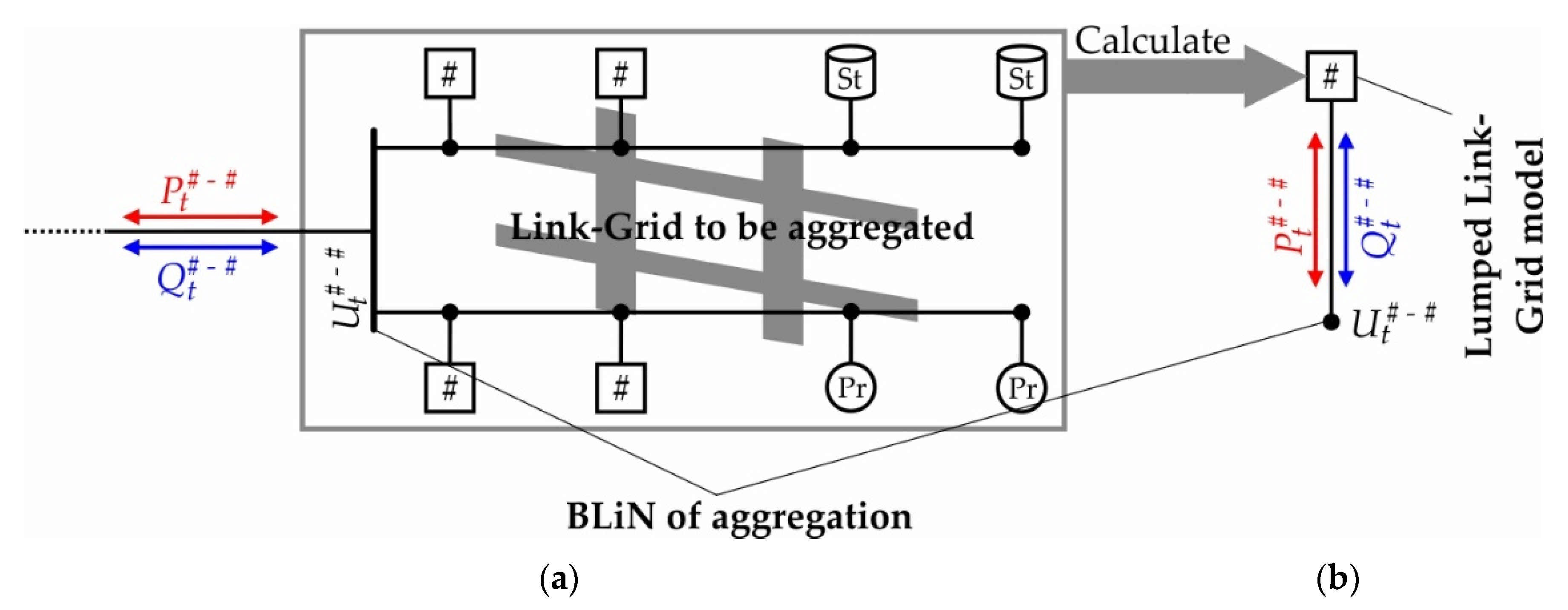
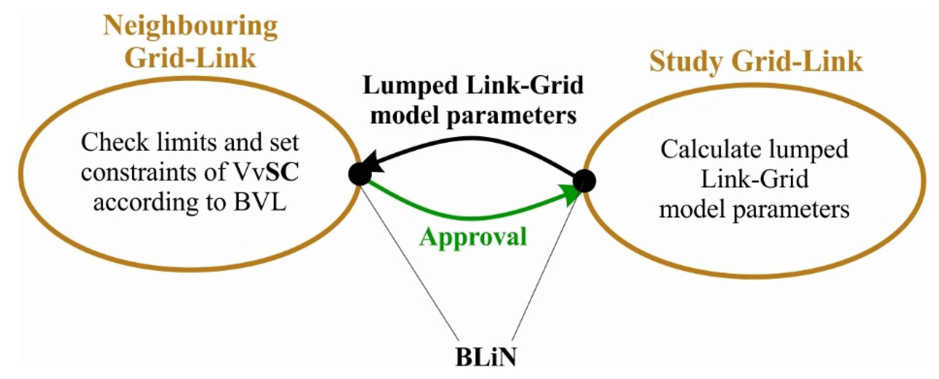
5.1.2. Calculation of Lumped Link-Grid Model Parameters
- Connect the slack node-element to the BLiN of aggregation.
- Define the slack voltage range of interest, e.g., from 0.9 p.u. to 1.1 p.u., and the corresponding resolution, e.g., 0.01 p.u. steps.
- Select one instant of time specified by the lumped models of the connected elements.
- Repeat load flow simulations of the selected instant of time for all defined slack voltages and record the P- and Q-values provided by the slack node-element. Furthermore, document all slack voltage values that provoke violations of the boundary voltage limits of any connected element.
- Repeat steps 1 to 4 for all other instants of time specified by the lumped models of the connected elements.
- The power contributions of the Link-Grid to be aggregated as functions of its boundary voltage;
- A set of slack voltage values that provoke violations of upper voltage limits at the boundary node of any connected lumped model. This set of values is denoted as , where k indexes the different values within this set;
- And a set of slack voltage values that provoke violations of lower voltage limits at the boundary node of any connected lumped model. This set of values is denoted as , where m indexes the different values within this set.
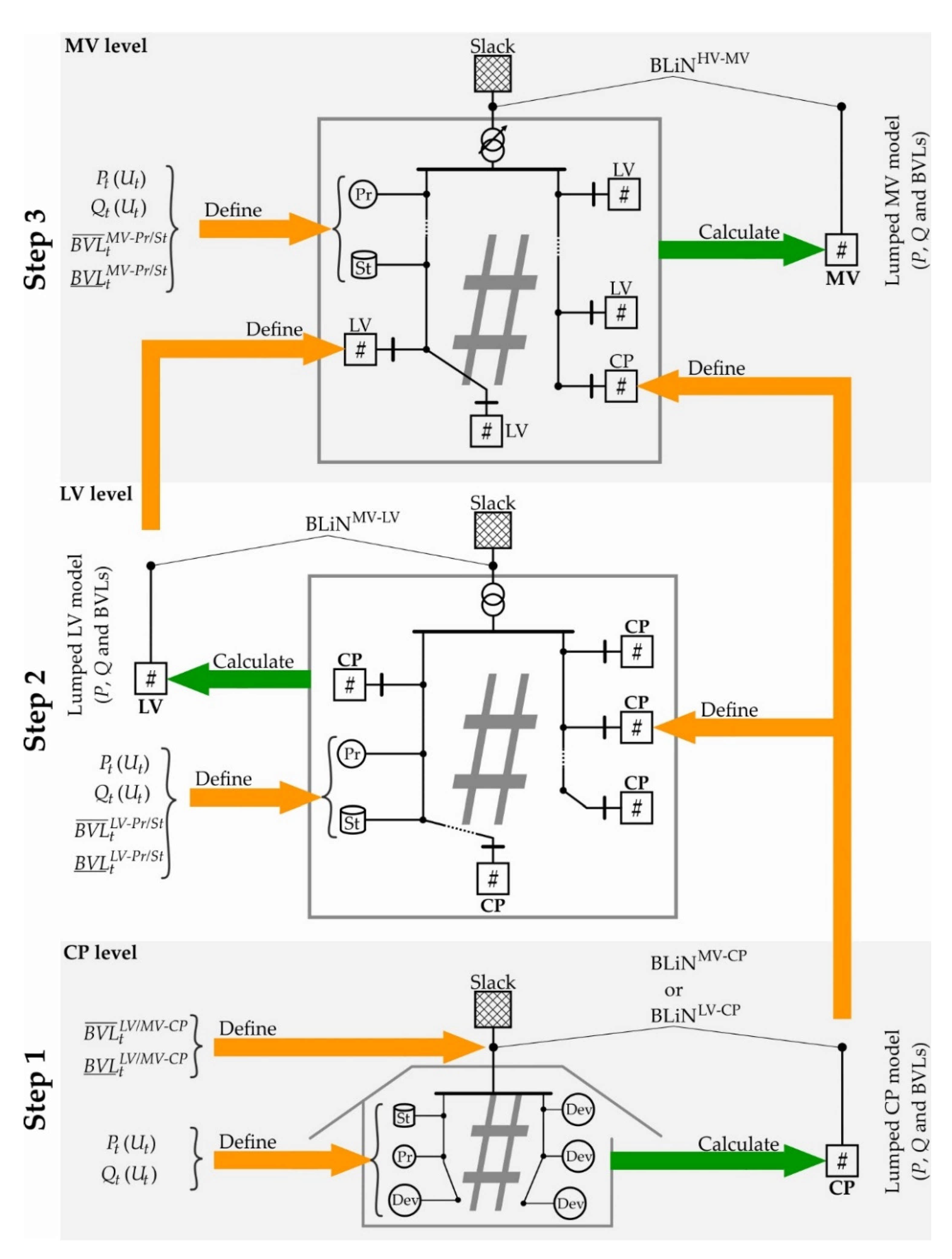
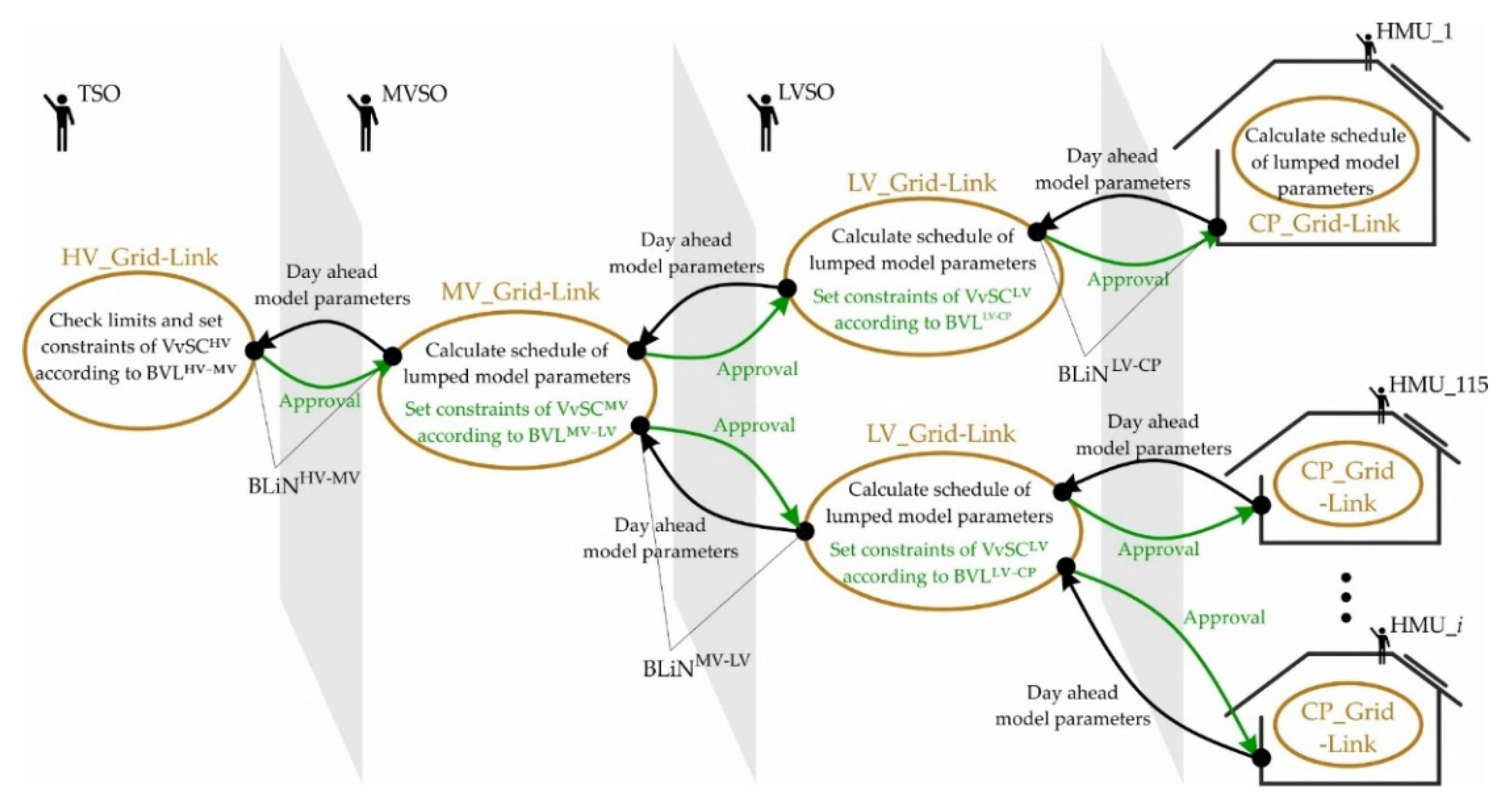
5.1.3. Chain Modeling in the Vertical Power System Axis
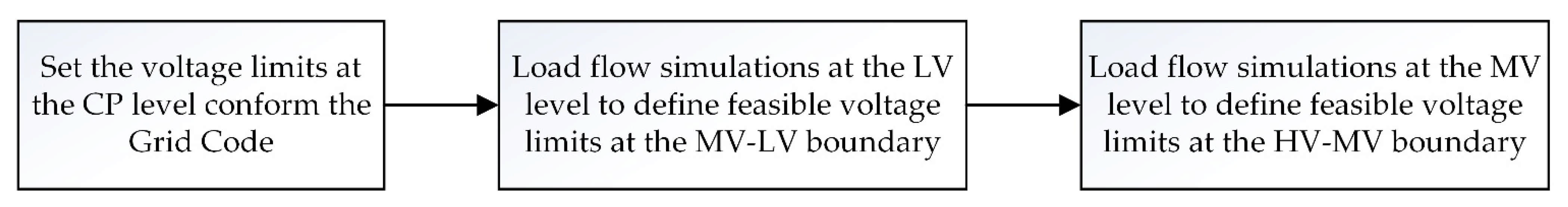
- The first step is to define the CP models, i.e., the structures of the CP_Link-Grids; The - and -behavior of the connected consuming devices, storages, and producers; the upper and lower LV–CP boundary voltage limits. These specifications allow analyzing the CP level and calculating the lumped CP_Link-Grid models according to the procedure described in Section 5.1.2.
- The next step is to analyze the LV level by representing the connected CPs by their lumped Link-Grid models and specifying the behavior and boundary voltage limits of producers and storages directly connected at the LV level. Again, the procedure described in Section 5.1.2 is used to calculate the lumped LV_Link-Grid models.
- Finally, the MV level is analyzed by representing the connected LV and CP_Link-Grids by their lumped Link-Grid models and by specifying the behavior and boundary voltage limits of the producers and storages directly connected at the MV level. The lumped MV_Link-Grid model can be calculated and provided for the analysis of the HV level.
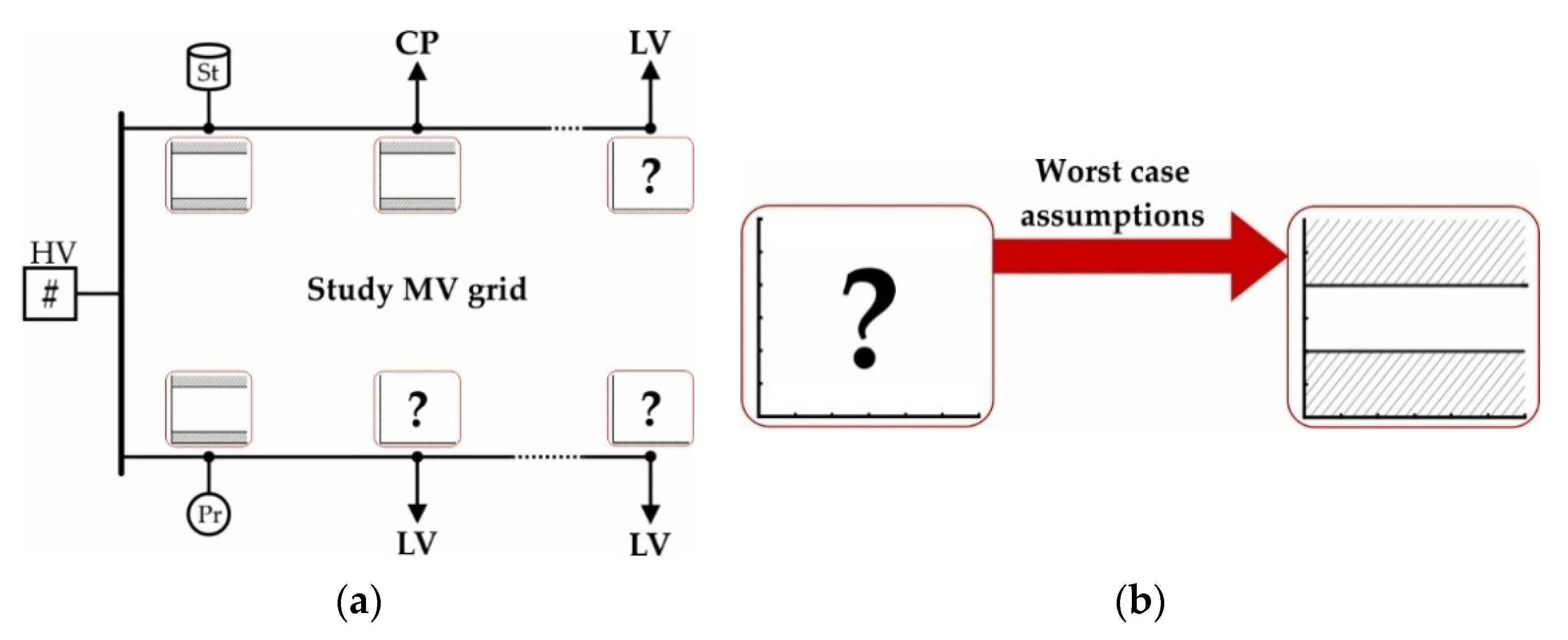
5.1.4. Validating Voltage Limit Compliance at the MV Level
5.2. Increasing the Infrastructure Utilization by Considering Boundary Voltage Limits
5.2.1. Generalized Use Case
5.2.2. Day-Ahead BVL Scheduling Chain
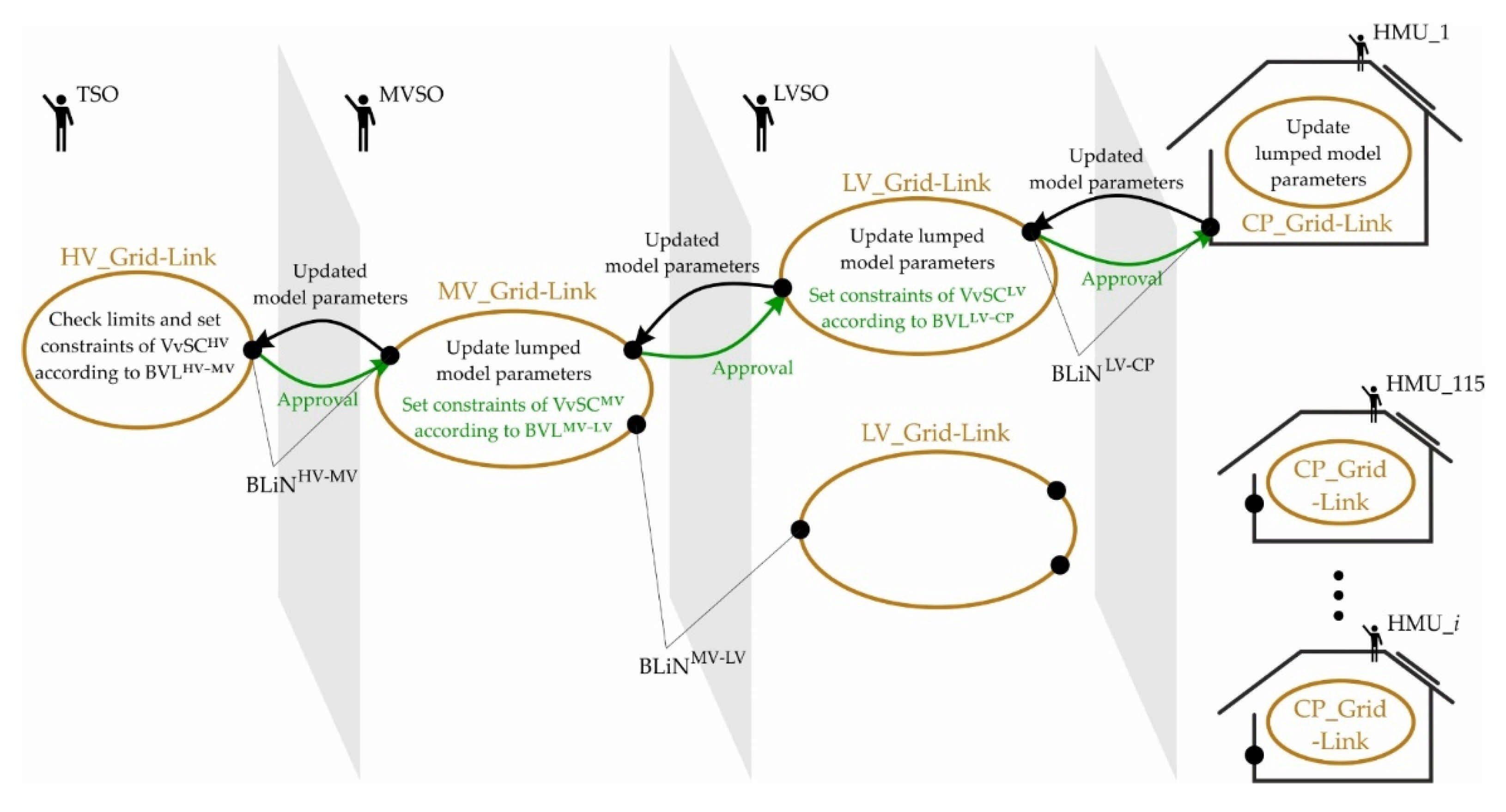
5.2.3. Short-Term BVL Adaptation Chain
5.3. New Functionalities for Load Flow Programs
- Automated calculation of the lumped Link-Grid model parameters
- The user defines the detailed model of the study Link-Grid and the lumped models (including boundary voltage limits) of the neighboring elements. The LF program automatically calculates the lumped model parameters of the study Link-Grid using the procedure described in Section 5.1.2.
- Automated lumped model creation for the calculation of neighboring Link-Grids
- The LF program uses the calculated parameters to generate the lumped Link-Grid model that can be used for the analysis of neighboring Link-Grids.
6. Conclusions
Author Contributions
Funding
Data Availability Statement
Conflicts of Interest
Appendix A
- Urban residential customer plant
- The urban residential CP, which is connected to the urban LV grid, equals the rural residential one except that the load profiles of the Dev.-model (see Figure 7b) are multiplied by the factor 1.43.
- Commercial customer plant
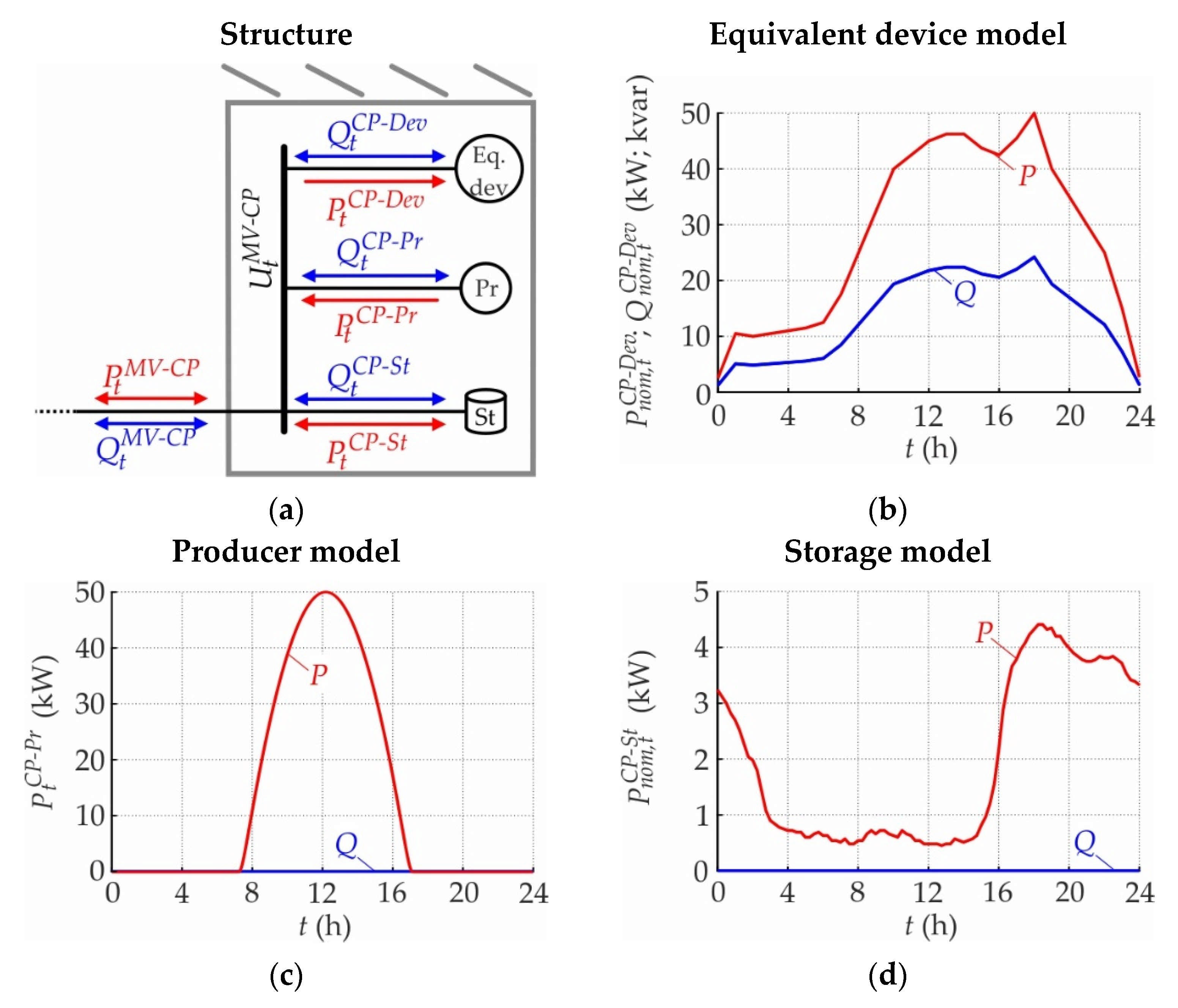
- The commercial CP is modeled as a single node—i.e., the BLiNMV-CP—connecting the Dev.-, Pr.-, and St.-models to the MV grid, Figure A1a. The active () and reactive power () exchanges between the MV grid and the commercial CP are determined by Equation (A1).
- Industrial CP
- The model of the industrial CP is connected to the MV grid and includes only the Dev.- and Pr.-models but not the St.-model, Figure A2a.

- Urban LV_Link-Grid
- Figure A3 shows the simplified one-line diagram of the urban LV grid with a nominal voltage of 0.4 kV. It is a real Austrian LV grid that includes nine feeders with a total line length of 12.815 km and a cable share of 96.14%. While the shortest feeder is 0.305 km in length, the longest one reaches 1.27 km. The feeders connect 175 urban residential CPs. The 20 kV/0.4 kV distribution transformer is rated with 800 kVA and has a total short circuit voltage of 4% with a resistive part of 1%. Its tap changer is fixed in mid-position. The MV–LV boundary node is set to the primary bus bar of the DTR, and the corresponding active and reactive power flows are designated as and , respectively.

Appendix B
Appendix C

| Abbreviation | Full Form | Abbreviation | Full Form |
|---|---|---|---|
| BLiN | Boundary link node | HV | High voltage |
| BPN | Boundary producer node | LF | Load flow |
| BSN | Boundary storage node | LV | Low voltage |
| BVL | Boundary voltage limit | LVSO | Low voltage system operator |
| COM | Component object model | MV | Medium voltage |
| CP | Customer plant | MVSO | Medium voltage system operator |
| Dev | Consuming device | OLTC | On-load tap changer |
| Dev.-model | Equivalent consuming device model | Pr | Producer |
| DP | Delivery point | Pr.-model | Producer model |
| DSO | Distribution system operator | PV | Photovoltaic |
| DTR | Distribution transformer | SC | Secondary control |
| EPO | Electricity producer operator | St | Storage |
| ESO | Electricity Storage operator | St.-model | Storage model |
| EV | Electric vehicle | TSO | Transmission system operator |
| HMU | Home management unit | VvSC | Volt/var secondary control |
| Variable | Meaning |
|---|---|
| # | Wildcard for any system level, i.e., HV, MV, LV, or CP |
| Upper boundary voltage limit of the lumped Link-Grid model i at t | |
| Lower boundary voltage limit of the lumped Link-Grid model i at t | |
| Upper boundary voltage limit of the Pr.-model i at t | |
| Lower boundary voltage limit of the Pr.-model i at t | |
| Upper boundary voltage limit of the St.-model i at t | |
| Lower boundary voltage limit of the St.-model i at t | |
| Reactive power constraint at the boundary node to the neighboring #_Link-Grid to be respected by the SC#. | |
| , , | Active power-related ZIP-coefficients of the Dev.-model at t |
| , , | Reactive power-related ZIP-coefficients of the Dev.-model at t |
| Active power exchange between Dev.-model and customer plant for nominal voltage at t | |
| Active power exchange between the St.-model and customer plant for nominal voltage at t | |
| Active power exchange between two Link-Grids at t | |
| Active power exchange between the Pr.-model and the connecting Link-Grid at t | |
| Active power exchange between the St.-model and the connecting Link-Grid at t | |
| Active power exchange between the Dev.-model and the customer plant at t | |
| Active power contribution of the slack element at t | |
| Reactive power exchange between the Dev.-model and customer plant for nominal voltage at t | |
| Reactive power exchange between the St.-model and customer plant for nominal voltage at t | |
| Reactive power exchange between two Link-Grids at t | |
| Active power exchange between the Pr.-model and the connecting Link-Grid at t | |
| Reactive power exchange between the St.-model and the connecting Link-Grid at t | |
| Reactive power exchange between the Dev.-model and the customer plant at t | |
| Reactive power contribution of the slack element at t | |
| Slack voltage value k that provokes violations of upper voltage limits at the boundary node of any connected lumped model at t | |
| Slack voltage value m that provokes violations of lower voltage limits at the boundary node of any connected lumped model at t | |
| Nominal voltage of the Link-Grid | |
| Boundary voltage between the Link-Grids at t | |
| Voltages within Link-Grids at t | |
| P | Active power |
| Q | Reactive power |
| t | Instant of time |
| U | Voltage |
References
- Ilo, A.; Gawlik, W. The Way from Traditional to Smart Power Systems. In Proceedings of the 9th IEWT, Vienna, Austria, 11–13 February 2015; pp. 1–7. [Google Scholar]
- Price, W.W.; Chiang, H.D.; Clark, H.K.; Concordia, C.; Lee, D.C.; Hsu, J.C.; Ihara, S.; King, C.A.; Lin, C.J.; Mansour, Y.; et al. Load Representation for Dynamic Performance Analysis (of Power Systems). IEEE Trans. Power Syst. 1993, 8, 472–482. [Google Scholar] [CrossRef]
- Arif, A.; Wang, Z.; Wang, J.; Mather, B.; Bashualdo, H.; Zhao, D. Load Modeling—A Review. IEEE Trans. Smart Grid 2018, 9, 5986–5999. [Google Scholar] [CrossRef]
- Modelling and Aggregation of Loads in Flexible Power Networks. Available online: https://e-cigre.org/publication/566-modelling-and-aggregation-of-loads-in-flexible-power-networks (accessed on 26 July 2021).
- Collin, A.J.; Tsagarakis, G.; Kiprakis, A.E.; McLaughlin, S. Development of Low-Voltage Load Models for the Residential Load Sector. IEEE Trans. Power Syst. 2014, 29, 2180–2188. [Google Scholar] [CrossRef]
- Lopes, J.A.P.; Hatziargyriou, N.; Mutale, J.; Djapic, P.; Jenkins, N. Integrating Distributed Generation into Electric Power Systems: A Review of Drivers, Challenges and Opportunities. Electr. Power Syst. Res. 2007, 77, 1189–1203. [Google Scholar] [CrossRef] [Green Version]
- Hatziargyriou, N.D.; Sakis Meliopoulos, A.P. Distributed Energy Sources: Technical Challenges. In Proceedings of the 2002 IEEE Power Engineering Society Winter Meeting, Conference Proceedings (Cat. No.02CH37309), New York, NY, USA, 27–31 January 2002; Volume 2, pp. 1017–1022. [Google Scholar]
- Manditereza, P.T.; Bansal, R. Renewable Distributed Generation: The Hidden Challenges—A Review from the Protection Perspective. Renew. Sustain. Energy Rev. 2016, 58, 1457–1465. [Google Scholar] [CrossRef]
- Yang, G.; Marra, F.; Juamperez, M.; Kjær, S.B.; Hashemi, S.; Østergaard, J.; Ipsen, H.H.; Frederiksen, K.H.B. Voltage Rise Mitigation for Solar PV Integration at LV Grids Studies from PVNET. Dk. J. Mod. Power Syst. Clean Energy 2015, 3, 411–421. [Google Scholar] [CrossRef] [Green Version]
- Bollen, M.H.J.; Sannino, A. Voltage Control with Inverter-Based Distributed Generation. IEEE Trans. Power Deliv. 2005, 20, 519–520. [Google Scholar] [CrossRef]
- Schweiger, G.; Eckerstorfer, L.V.; Hafner, I.; Fleischhacker, A.; Radl, J.; Glock, B.; Wastian, M.; Rößler, M.; Lettner, G.; Popper, N.; et al. Active Consumer Participation in Smart Energy Systems. Energy Build. 2020, 227, 110359. [Google Scholar] [CrossRef]
- Myrda, P.; Mcgranaghan, M. Smart Grid Enabled Asset Management. In Proceedings of the CIRED Workshop, Lyon, France, 7–8 June 2010; pp. 1–4. [Google Scholar]
- Cárdenas, A.A.; Safavi-Naini, R. Chapter 25—Security and Privacy in the Smart Grid. In Handbook on Securing Cyber-Physical Critical Infrastructure; Das, S.K., Kant, K., Zhang, N., Eds.; Morgan Kaufmann: Boston, MA, USA, 2012; pp. 637–654. ISBN 978-0-12-415815-3. [Google Scholar]
- Vaahedi, E. Practical Power System Operation, 1st ed.; John Wiley & Sons, Ltd.: Hoboken, NJ, USA, 2014. [Google Scholar]
- O’Connell, N.; Pinson, P.; Madsen, H.; O’Malley, M. Benefits and Challenges of Electrical Demand Response: A Critical Review. Renew. Sustain. Energy Rev. 2014, 39, 686–699. [Google Scholar] [CrossRef]
- Guo, Q.; Qi, J.; Ajjarapu, V.; Bravo, R.; Chow, J.; Li, Z.; Moghe, R.; Nasr-Azadani, E.; Tamrakar, U.; Taranto, G.N.; et al. Review of Challenges and Research Opportunities for Voltage Control in Smart Grids. IEEE Trans. Power Syst. 2019, 34, 2790–2801. [Google Scholar] [CrossRef] [Green Version]
- Ilo, A. Design of the Smart Grid Architecture According to Fractal Principles and the Basics of Corresponding Market Structure. Energies 2019, 12, 4153. [Google Scholar] [CrossRef] [Green Version]
- Ilo, A. “Link”—The Smart Grid Paradigm for a Secure Decentralized Operation Architecture. Electr. Power Syst. Res. 2016, 131, 116–125. [Google Scholar] [CrossRef]
- DIN EN 50160:2020-11 Merkmale Der Spannung in Öffentlichen Elektrizitätsversorgungsnetzen; Deutsche Fassung EN_50160:2010_ + Cor.:2010_ + A1:2015_ + A2:2019_ + A3:2019; Beuth Verlag GmbH: Berlin, Germany, 2020.
- Hashemi, S.; Østergaard, J. Methods and Strategies for Overvoltage Prevention in Low Voltage Distribution Systems with PV. IET Renew. Power Gener. 2016, 11. [Google Scholar] [CrossRef] [Green Version]
- PSS®SINCAL—Simulation Software for Analysis and Planning of All Network Types. Available online: https://new.siemens.com/global/en/products/energy/energy-automation-and-smart-grid/pss-software/pss-sincal.html (accessed on 13 August 2021).
- MATLAB—MathWorks. Available online: https://de.mathworks.com/products/matlab.html (accessed on 13 August 2021).
- Ilo, A. The Energy Supply Chain Net. Energy Power Eng. 2013, 05, 384–390. [Google Scholar] [CrossRef] [Green Version]
- Schultis, D.-L.; Ilo, A. TUWien_LV_TestGrids. Mendeley Data 2018, 1. [Google Scholar] [CrossRef]
- Schultis, D.-L. Daily Load Profiles and ZIP Models of Current and New Residential Customers. Mendeley Data 2019, 1. [Google Scholar] [CrossRef]
- Schultis, D.-L.; Ilo, A. Adaption of the Current Load Model to Consider Residential Customers Having Turned to LED Lighting. In Proceedings of the 2019 IEEE PES Asia-Pacific Power and Energy Engineering Conference (APPEEC), Macao, China, 1–4 December 2019; pp. 1–5. [Google Scholar]
- Shukla, A.; Verma, K.; Kumar, R. Multi-Stage Voltage Dependent Load Modelling of Fast Charging Electric Vehicle. In Proceedings of the 2017 6th International Conference on Computer Applications In Electrical Engineering-Recent Advances (CERA), Roorkee, India, 5–7 October 2017; pp. 86–91. [Google Scholar]
- Aunedi, M.; Woolf, M.; Strbac, G.; Babalola, O.; Clark, M. Characteristic Demand Profiles of Residential and Commercial EV Users and Opportunities for Smart Charging. In Proceedings of the 23rd International Conference on Electricity Distribution (CIRED 2015), Lyon, France, 15–18 June 2015; pp. 1–5. [Google Scholar]
- Ilo, A. Demand Response Process in Context of the Unified LINK-Based Architecture; Springer International Publishing: Basel, Switzerland, 2018; pp. 75–83. [Google Scholar]
- Bokhari, A.; Alkan, A.; Dogan, R.; Diaz-Aguiló, M.; de León, F.; Czarkowski, D.; Zabar, Z.; Birenbaum, L.; Noel, A.; Uosef, R.E. Experimental Determination of the ZIP Coefficients for Modern Residential, Commercial, and Industrial Loads. IEEE Trans. Power Deliv. 2014, 29, 1372–1381. [Google Scholar] [CrossRef]
- Benchmark Systems for Network Integration of Renewable and Distributed Energy Resources. Available online: https://e-cigre.org/publication/ELT_273_8-benchmark-systems-for-network-integration-of-renewable-and-distributed-energy-resources (accessed on 26 July 2021).


Publisher’s Note: MDPI stays neutral with regard to jurisdictional claims in published maps and institutional affiliations. |
© 2021 by the authors. Licensee MDPI, Basel, Switzerland. This article is an open access article distributed under the terms and conditions of the Creative Commons Attribution (CC BY) license (https://creativecommons.org/licenses/by/4.0/).
Share and Cite
Schultis, D.-L.; Ilo, A. Increasing the Utilization of Existing Infrastructures by Using the Newly Introduced Boundary Voltage Limits. Energies 2021, 14, 5106. https://doi.org/10.3390/en14165106
Schultis D-L, Ilo A. Increasing the Utilization of Existing Infrastructures by Using the Newly Introduced Boundary Voltage Limits. Energies. 2021; 14(16):5106. https://doi.org/10.3390/en14165106
Chicago/Turabian StyleSchultis, Daniel-Leon, and Albana Ilo. 2021. "Increasing the Utilization of Existing Infrastructures by Using the Newly Introduced Boundary Voltage Limits" Energies 14, no. 16: 5106. https://doi.org/10.3390/en14165106