Transient Stability Analysis of a Transmission Network Using Eigenvalue Principles with Automated VAR Compensation: A Case Study of the Nigerian Eastern Grid

Abstract

Power systems may encounter disturbances during operation as a result of switching of various components, etc. Such perturbations include transformer tap-changing action, load variations, and line outages due to various types of faults of which an earth fault is the most common. Stability analysis of a transmission system is necessary for us to determine the stability state of the system so that appropriate control measures can be implemented to guarantee system stability. This article presents the use of eigenvalue obtained from the system-linearized eigenvectors to analyze the stability state of the system. The choice of the eigenvalue principle is based on the strength of accuracy of the method to determine the actual state of the system providing adequate data for easy solution to the problem. The node admittance parameters computed from the line parameters is applied to the eigenvalue–eigenvector model to determine the system stability state. The state of the eigenvalue is used as an input to a control system, which utilized static volt-ampere reactive (VAR) compensators (SVC) to automatically stabilize the non-stable buses in the transmission network. The 6 × 6 nodal admittance matrix is formed and fed to the developed eigenvalue–eigenvector model via MATLAB in order to compute the right and left eigenvectors and the diagonal or eigenvalue of the network under steady-state and contingency condition. After this, the system stability state is determined, and necessary control actions by the SVC are implemented to guarantee system security. The developed model was tested on the 6 bus Eastern Grid Nigerian Transmission Network and validated using a 41 bus network of the same country. The compensated model showed considerable efficiency in improving the transient stability state of the transmission networks in terms of ease of operation, seamless integration into existing control system, and efficient utilization of SVS to compensate for reactive power imbalances. The results from the step response graph of the compensated model shows performance accuracy as the system regained stability in less than 0.5 s, which is a significant improvement over the uncompensated model.

1. Introduction

Owing to diverse loads with various short circuit capacities scattered in the power system, operation disturbances are almost inevitable. Sudden loss of generators, high-capacity line outage, or heavy short circuits resulting from equipment breakdown or lightning strikes constitutes large disturbances encountered in the power system. Small burdens occur due to load variations and equipment switching such as tap-changing transformer actions. All these cause the power system to experience instability or transient state which is of important note to power system engineers [1]. It is paramount that the power system maintain synchronism. The large size of transmission network makes the associated transient fizzle out quickly; therefore, it is usually neglected. Consequently, the consideration and emphasis of many transient stability studies are on the distribution network and generator oscillations. However, a further assessment of the effect of small oscillation or any form of transient in the transmission network has necessitated further dimensions in transient analysis and advancement in technologies capable of damping out small oscillation or compensating variations. Optimal placement and utilization of flexible alternating current transmission system (FACTS) devices have been considered for transmission network transient stability [2,3,4]. A comparative study of unifying the power flow controller (UPFC) and interline power flow controller (IPFC) shows the effectiveness of these devices in stabilizing transient in transmission networks [2,3,4]. Modal or eigenvalue investigation of small-signal power system stability was swiftly analyzed and presented in [5]. The study analyzed the insecurity issues of an inter-area mode swing and suggested a power system stabilizer (PSS) location based on the result of the analysis. It was suggested that the use of high-voltage direct current (HVDC) and FACTS devices improves system dynamics and stability with their ability to change the power flow directly and indirectly within milliseconds. The effect of small disturbances on system stability was investigated in [6] to decide the best position for PSS, to reinstate system stability by evaluating the eigenvalue and eigenvectors of the linearized differential and algebraic equation of the system. The results suggested optimal placement of PSS for transient stability. Halder et al. [7] presented a novel non-linear control scheme for thyristor-controlled series capacitors (TCSCs), formulated by the zero dynamic design approach for transient stability analysis of a multi-machine power system. The results showed that such a model is more effective in terms of performance characteristics under different loading conditions when applied to a 14-areas, 24-machines, and 203-buses model. The effect of an adaptive neuro-fuzzy inference system (ANFIS)-based UPFC in a wind–diesel system and doubly fed induction generator DFIG-based wind turbine system using a small signal model was examined in [8]. The authors carried out simulation in MATLAB with different wind power input and a 2% step increase in load demand. The result of the analysis illustrated the efficiency and effectiveness of their approach and its impact on transient behavior of the micro-grid. Madruga et al. [9] suggested a methodology that would be suitable for distribution network transient analysis using a simple distribution network model. Different disturbance types and buses were selected for application with the adjustment of stability control systems. This method is suitable for unbalanced networks and demonstrated a single-pole switching using a real network as a case study. The small signal stability of a large power system using Krylov subspace technique was examined by [10].

Furthermore, different approaches have been adopted in transient stability analysis considering response time and performance accuracy. An algorithm based on the implicitly restarted Arnoldi method coupled with the dynamic switching approach was adapted and implemented a transmission network. The result of their analysis showed proper convergence to the sought eigenvalues, though with poor damping. Cho et al. [11] developed a novel approach capable of dealing with time-domain simulation for dynamic stability studies and operation of large-scale power systems. They further proposed a new model to overcome the low-voltage problem, which provided a good performance and convergence when the terminal voltage is below some predefined value. In comparison to commercial tools, the solution was found to be numerically well conditioned by the introduction of ZIP model algorithm. Marchiori et al. [12] presented a methodology to analyze an electric power system’s transient stability for first swing using a neural network based on adaptive resonance theory (ART) architecture, called Euclidean ARTMAP neural network. The proposed neural network was applied to a multi-machine electric power system composed of 10 synchronous machines, 45 buses, and 73 transmission lines. In comparison with a ARTMAP fuzzy-type model, it provided a faster and a more accurate solution. The solution allows us to approach several topologies of an electric system at the same time; therefore, it is an alternative to real-time transient stability of electric power systems. Additionally, Izumi et al. [13] analyzed the transient stability of power systems using sum of squares programming, considering machine inertia and damping coefficients as uncertain parameters, using polytopic representation for uncertain parameters and a concept from the field of robust control. The method proves that the sum of square programming is feasible in this context and, hence, was used to solve the analyses problem of robust transient stability using a numerical example. Xu et al. [14] studied the method of analyzing electric network resonance stability (ENRS), with the main objective of establishing a systematic approach to solving the problem. The s-domain nodal admittance matrix (NAM) of the electric network was introduced and used to transform the judgment of ENRS into the zero-point solution of the determinant of the s-domain NAM. First, it was proven that the zero points of the determinant of the s-domain NAM are equivalent to the system eigenvalues. Then, they further identified the dominant resonance region and determined the key components related to resonance nodes with reference to the eigenvalues of the system.

The use of eigenvectors corresponding to the power system oscillatory modes was used to determine the relative motions of the machines at this mode and to find out which machines were swinging with and against each other in [15]. A hybrid BBO-DE with an eigenvalue analysis-based optimization problem was presented in [16]. The proposed algorithm was tested on an IEEE system with 10 generators and 19 load centers considering 2.0 s fault time and 2.50 s clearing time. The results obtained determined which machine is the candidate for power system stabilizer (PSS) placement. In [17], a comparative report of eigenvalue tracking (ET), participation factor (PF), and residual (RES) was presented, as well as methods for determining PSS placement among the generators in order to achieve stable operation. It was noted that ET methods showed better performance than the other methods compared.

The motivation behind this work is that small signal oscillation is usually overlooked in transmission network owing to the idea that when such transient occurs, it dies out on its own without regulations because of the large nature of transmission networks. These neglected small signal oscillations do exit and, over time, cause a breakdown of network components. To identify the existence of these transient in a transmission network system, the eigenvalue principle, as the most classical mathematical approach, is appreciated for its high accuracy and has been used in several studies to determine such small oscillation in the distribution network or for optimal placement of FACTS devices [15,16,17]. This article proposes the utilization of the eigenvalue principle for clear cut details of the stability state of the transmission network in order to provide the needed control measures as efficiently as possible. As compared to other methods, the integration of eigenvalues into the space state for effective control is easy, and the idea of regulating the use of VAR compensation makes it more efficient than traditional methods of permanently placing a FACTS device in the system without adequate regulation.

A further review of the already existing literature shows that most research work carried out on power system stability majorly focused on the generators and the buses at which they are connected, with reference to local and inter-area oscillation of generators. In this article, we present transmission network stability analysis using eigenvalue calculated from the system linearized eigenvectors. The node admittance parameters computed from the line parameters is applied to the eigenvalue–eigenvector model to determine the system stability state, and the automated compensation scheme (SVS) is incorporated into the system to improve its transient stability by providing the required reactive power compensation. This is an extension of transmission network stability analysis based on eigenvalue carried out in [18]. The eigenvalue model developed in this article is multi-machine compliant and operates in real time, utilizing obtained data at the supervisory control and data acquisition (SCADA) to compute the system eigenvalue with which it performs automatic compensation of the transmission network. The significance of this proposed model is the performance accuracy of the model in determining the system steady state and quick response time in restoring stability. The sequence of this paper is such that Section 2 presents model formulation that involves eigenvalue analysis and modification to include VAR compensation, Section 3 details application in case studies, while Section 4 presents and discusses the results, and Section 5 concludes the study.

2. Materials and Methods

For the analysis of balanced conditions, a single-phase representation of the three-phases model is used. Without the balanced steady-state representation of the transmission network, stability analysis of large practical power systems would be difficult. Electromagnetic transient programs (EMTP) are used for complex transient stability analysis involving generators, stators, and network transients [19]. For conventional transient stability analysis, the network representation is similar to that for power-flow analysis. For the purpose of this analysis, nodal admittance matrices shall be used. In loads modeling, dynamic loads are represented as induction and synchronous motors, and they are treated as synchronous machines. Static loads are represented as part of the network equations. Network loads with invariable impedance characteristics are the easiest to handle and are incorporated in the node admittance matrix. Nonlinear loads are modeled as a polynomial or exponential function of bus voltage magnitude and frequency [1]. This is represented as a current injection at the appropriate node in the network equation. 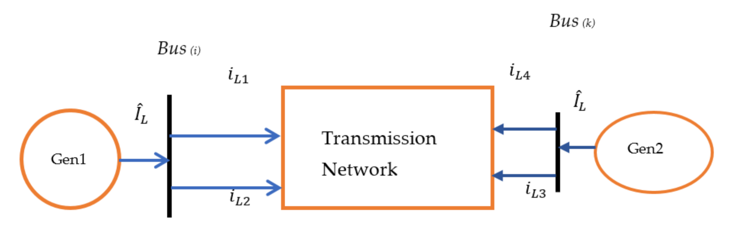Figure 1 shows a classic power system network in modular form.

The value of the node current injected${\widehat{I}}_L$ into the network is the sum of the branch currents $i_{L1} \mathrm{and} i_{L2}$.

$${\widehat{I}}_L=i_{L1}+i_{L2}=-\frac{P_L-Q_L}{\widehat{V^{*}{}_L}}$$

(1)

where ${\widehat{V}}^{*}{}_L$ is the conjugate of the load bus voltage, P_L and Q_L are segments of the active and reactive components of the load, which vary as nonlinear functions of V_L and Frequency deviation. For an inductive load, Q_L is positive.

The overall network/load representation comprises a large sparse nodal admittance matrix equation with a structure similar to that of the power-flow problem. The network equation is written in matrix form as:

$${\widehat{I}}_L=Y_N\widehat{V}$$

(2)

The node admittance matrix $Y_N$ is symmetrical, except for dissymmetry introduced by phase-shifting transformers. Within the time frame of transient stability simulations, transformer taps and phase-shift angles do not change. Therefore, the elements of the matrix remain constant except for change introduced by network switching operations or external loads. The effect of generators, nonlinear static loads, dynamic loads, and other devices such as HVDC converters and regulated VAR compensators are reflected as boundary conditions providing additional relationships between voltages $\widehat{V} \mathrm{and} \mathrm{currents} \widehat{I}$ at the respective nodes. In contrast to power-flow analysis, tie line power-flow control, limits on generator reactive power output, and the slack bus make up for the unknown losses and need not be considered in transient stability analysis [1].

For (k^th) number of buses, $Y_{bus}$ can be expressed as

$$\frac{1}{ Z_{bus}}=\frac{1}{r\pm jx}=Y_{bus}=\left[\begin{array}{c}\begin{array}{ccc}{Y}_{11}& Y_{12}& \dots Y_{1i}\\ Y_{21}& Y_{22}& \dots Y_{2i}\\ Y_{31}& Y_{32}& \dots Y_{3i}\end{array}\\ \begin{array}{ccc}⋮ & ⋮& \dots \end{array}\dot{⋮}\\ \begin{array}{ccc}{Y}_{k1}& Y_{k2}& \dots \end{array}{Y}_{kk}\end{array}\right]$$

(3)

The off diagonal elements of the matrix are called mutual admittances, while the diagonal elements are called self-admittances. $r\pm jx$ represent the branch resistances and reactance, respectively. Equation (4) defines the mutual admittance and expressed it as the negative of the admittance of the line between buses$1$ and $k$, while Equation (5) defines the self-admittance as the sum of all the admittances connected to the bus under consideration.

$$Y_{i1}=Y_{1i}=-y_{i1}=-y_{1i}$$

(4)

$$Y_{ii}={\displaystyle \sum }_{\begin{array}{c}i=0\\ i\ne 1\end{array}}^n{y}_{ii}$$

(5)

2.1. Eigenvalue Analysis

Equation (2) can be written in steady-state space form as:

$$Ax=\widehat{x}$$

(6)

In order to obtain the solution of Equation (6), a scalar parameter $\lambda$ called the eigenvalue is introduced such that Equation (6) becomes

$$Ax=\lambda x$$

(7)

where $A=\left[a_{k1}\right]$an n × n square matrix, $x$ is an n × 1 vector, and $\lambda$ is a scalar parameter [1,20]. Therefore, the solution $x=0$ for $\lambda$ is indeed not useful and, thus, is neglected.

For non-trivial solutions, i.e.,$x\ne 0$, the values of $\lambda$ are known as the eigenvalues and the characteristics values or underlying roots of the matrix A, and the matching solutions of Equation (7) are called eigenvectors or attribute vectors of A. When written as separate equations we have

$$A.x-\lambda x=0$$

(8)

$$\left(A-\lambda I\right)x=0$$

(9)

It is noteworthy that the unit matrix $I$was introduced so that $\lambda$ can be deducted from matrix A. Now, for Equation (9) to have a non-trial solution, the determinant of $\left|A-\lambda I\right|$ must be equal to zero. Hence

$$\left|A-\lambda I\right|=\left|\begin{array}{cccc}\left(a_{11}-\lambda \right)& a_{12}& \cdots & a_{1i}\\ a_{21}& \left(a_{22}-\lambda \right)& \cdots & a_{2i}\\ ⋮& ⋮& \dots & ⋮\\ a_{k1}& a_{k2}& \dots & \left(a_{kk}-\lambda \right)\end{array}\right|=0$$

(10)

Expansion of Equation (10) gives the characteristics equation. The n solutions of $\lambda ={\lambda }_1, {\lambda }_2, {\lambda }_{3,}\dots .{\lambda }_n$ are eigenvalues of A.

2.2. Modified Eigenvalue with VAR Compensation Model

From the general form of state-space representation of a linear time-invariant system [21] shown in Equations (11) and (12) whose closed-loop system block diagram is shown in Figure 2, we derive the eigenvalue transmission network-compensated mathematical model based on double-stage state feedback control law.

$$\dot{x}\left(t\right)=Ax\left(t\right)+Bu\left(t\right)$$

(11)

$$y\left(t\right)=Cx\left(t\right)+Du\left(t\right)$$

(12)

where $\dot{x}\left(t\right)$ is the input variable vector, $Ax\left(t\right)$ is the state space variable of the input state, $Bu\left(t\right)$ is the input variable gain parameter, while $y\left(t\right)$ is the output variable vector, $Cx\left(t\right)$ is the state space variable of the output state, $Du\left(t\right)$ is the output feed-forward gain, and $x\left(t_0\right)=x_0$is the initial condition of the input variable.

With the application of state feedback control law of the form (13), the unit input signal $u\left(t\right)$is

$$u\left(t\right)=-Kx\left(t\right)+r\left(t\right)$$

(13)

With $Kx\left(t\right)$ as feedback control state and $r\left(t\right)$ as biasing input signal.

The new network state of the transmission network at time (t) represented by Equations (11) and (12) becomes

$$\dot{x}\left(t\right)=\left(A-BK\right)x\left(t\right)+Br\left(t\right)$$

(14)

This features a constant state feedback gain matrix K of dimension m × n and a new external reference input r(t) having the same dimension m × 1 as the open-loop input u(t) and the same physical features.

With reference to eigenvalue formulation developed in this article in Section 2.1, we derive the eigenvalue transmission network compensated model as represented in Figure 3 as follows

$$u\left(t\right)=-Iv\left(t\right)+r\left(t\right)$$

(15)

$$i\left(t\right)=\left(Y_N-\lambda I\right)v\left(t\right)+Br\left(t\right)$$

(16)

$$y\left(t\right)=Cv\left(t\right)+Du\left(t\right)$$

(17)

To implement the automatic compensation of the transmission network, the output y(t) is fed into the SCADA system. The SCADA system, as the meaning implies, is a supervisory control and data acquisition system; hence, it is where eigenvalue processor signal is computed utilizing the output data feed in from the network. This unit modifies the output control signal as follows

$$y\left(t\right)=\left(C-DI\right)v\left(t\right)+Dr\left(t\right)+\mathsf{{\rm E}}r\left(t\right)$$

(18)

where $\mathsf{{\rm E}}r\left(t\right)$ represents SVC input to the system to obtain a stable output as represented in Figure 4.

Additionally, the frequencies of oscillation given by the imaginary part divided by $2\pi$ produced values in the range of 1 to 2 Hz, the flicker causative frequency. To this effect, we propose a voltage swing control system, which could monitor the resultant eigenvalues computed based on the condition of a given power system transmission network and actuate the necessary compensation scheme, in this case, SVC. The proposed model as discussed in Section 2.2 is illustrated in modular form in Figure 5.

The transmission network parameters are read in real time using SCADA, then the eigenvalues are computed and the real and the imaginary part extracted. The eigenvalue processor will determine if the values are negative or positive and perform the necessary actuation operation. The installed static VAR compensators are automatically switched in and out of the network based on the transient state of the network determined by the eigenvalue model result.

2.3. Application to 330 kV Nigerian Eastern Grid Network (EG-N)

The Nigerian prototype Eastern Grid Network is as shown in Figure 6. The network is made of 6 buses and 3 generators. The external loads connected to the bus are not incorporated into the analysis. Double line circuits were treated as parallel circuits to determine their equivalent reactance. A resistance component of the network data was also neglected.

For the rationale of eigenvalue analysis, we contrast Equation (2) ${\widehat{I}}_L=Y_N\widehat{V}$ and (6) $Ax=\widehat{x}$and derive the network nodal admittance matrix Y from data obtained from the Nigerian transmission company, Oshogbo, as presented in

Table 1. Network data [22].

S/NO	LINE-FROM	LINE-TO	TYPE	R	X
1	Ugwuaji (6)	New Haven (4)	Double	0.0394	0.303
2	Onitsha (5)	New Haven (4)	Double	0.039	0.331
3	Okpai (1)	Onitsha (5)	Double	0.0394	0.303
4	Delta PS (3)	Onitsha (5)	Single	0.039	0.331
5	Onitsha (5)	Alaoji (2)	Single	0.039	0.331

.

Let ${\widehat{I}}_L=\widehat{x}$, $\widehat{V}=x$, and $Y_N=A.$Then, it follows that Equation (9) holds true for

$$\left(Y_N-\lambda I\right)\widehat{V}=0$$

(19)

Writing Equation (19) in determinant form gives

$$\left|Y_N-\lambda I\right|=\left|\begin{array}{cccc}\left(y_{11}-\lambda \right)& y_{12}& \cdots & y_{1i}\\ y_{21}& \left(y_{22}-\lambda \right)& \cdots & y_{2i}\\ ⋮& ⋮& \dots & ⋮\\ y_{k1}& y_{k2}& \dots & \left(y_{kk}-\lambda \right)\end{array}\right|=0$$

(20)

The network admittance $Y_N$can be obtained as shown below:

$$y_{11\left(Okpai\right)}=\sum \left[2\left(y_{15}\right)\right]=2\left(\frac{1}{0.0394+j0.303}\right)=0.844-j6.491$$

(21)

$$y_{22\left(Alaoji\right)}=\sum \left[y_{25}\right]=\frac{1}{0.039+j0.331}=0.351-j2.980$$

(22)

$$y_{33\left(Delta PS\right)}=\sum \left[y_{35}\right]=\frac{1}{0.039+j0.331}=0.351-j2.98$$

(23)

$$y_{44\left(New Haven\right)}=\sum \left[2\left(y_{45}\right)+2\left(y_{46}\right)\right]=1.546+j0.531$$

(24)

$$y_{55\left(Onitsha\right)}=\sum \left[y_{53}+2\left(y_{51}\right)+y_{52}+y_{54}\right]=2.248+j18.411$$

(25)

$$y_{66\left(Ugwuaji\right)}=\sum \left[2\left(y_{64}\right)\right]=0.844-j6.491$$

(26)

$$Y_N=\left[\begin{array}{cccccc}\hfill y_{11}\hfill & \hfill y_{12}\hfill & \hfill y_{13}\hfill & y_{14}\hfill & \hfill y_{15}\hfill & \hfill y_{16}\hfill \\ \hfill y_{21}\hfill & \hfill y_{22}\hfill & \hfill y_{23}\hfill & y_{24}\hfill & \hfill y_{25}\hfill & \hfill y_{26}\hfill \\ \hfill y_{31}\hfill & \hfill y_{32}\hfill & \hfill y_{33}\hfill & y_{34}\hfill & \hfill y_{35}\hfill & \hfill y_{36}\hfill \\ \hfill y_{41}\hfill & \hfill y_{42}\hfill & \hfill y_{43}\hfill & y_{44}\hfill & \hfill y_{45}\hfill & \hfill y_{46}\hfill \\ \hfill y_{51}\hfill & \hfill y_{52}\hfill & \hfill y_{53}\hfill & y_{54}\hfill & \hfill y_{55}\hfill & \hfill y_{56}\hfill \\ \hfill y_{61}\hfill & \hfill y_{62}\hfill & \hfill y_{63}\hfill & y_{64}\hfill & \hfill y_{65}\hfill & \hfill y_{66}\hfill \end{array}\right]$$

(27)

Therefore,

$${\mathit{Y}}_{\mathit{N}}=\left|\begin{array}{cccccc}0.841-j6.491\hfill & -0\hfill & -0\hfill & -0\hfill & -0.422+j3.245\hfill & -0\hfill \\ -0\hfill & 0.351-j2.980\hfill & -0\hfill & -0\hfill & -0.351+j2.980\hfill & -0\hfill \\ -0\hfill & -0\hfill & 0.351-j2.980\hfill & -0\hfill & 0.351+j2.980\hfill & -0\hfill \\ -0\hfill & -0\hfill & -0\hfill & 1.546+j0.531\hfill & -0.351+j2.980\hfill & -0.422+j3.245\hfill \\ -0.422+j3.245\hfill & -0.351+j2.980\hfill & -0.351+j2.980\hfill & -0.351+j2.980\hfill & 2.248+j3.411\hfill & -0\hfill \\ -0\hfill & -0\hfill & -0\hfill & -0.422+j3.245\hfill & -0\hfill & 0.844-j6.491\hfill \end{array}\right|$$

(28)

The 6 × 6 matrix of Equation (21) was coded into the MATLAB workplace command prompt, and the right eigenvector (V = ${\widehat{I}}_L$), the eigenvalues (D = $\lambda$), and the left eigenvector (W = $\widehat{ V}$) were computed and the results are presented in the next section.

3. Result of Transient Analysis of 6 Bus Eastern Nigerian Network

The term right eigenvector, eigenvalues, and left eigenvector are built in variables, which MATLAB assigns to vector matrices. These terms are synonymous with the variables used in the analysis as represented in

Table 2. Right eigenvector (V = ${\widehat{I}}_L$).

0.6263 + 0.0000i	−0.4117 + 0.0341i	0.6374 + 0.0000i	0.1304 + 0.0500i	0.0686 − 0.0470i	−0.0000 + 0.0000i
0.1439 + 0.0023i	−0.0434 − 0.0036i	−0.2375 − 0.0895i	0.5578 + 0.0000i	−0.3253 − 0.0196i	−0.7070 + 0.0000i
0.1439 + 0.0023i	−0.0434 − 0.0036i	−0.2375 − 0.0896i	0.5577 − 0.0002i	−0.3252 − 0.0197i	0.7072 + 0.0000i
0.3095 + 0.0049i	0.3149 + 0.0069i	−0.2480 − 0.0387i	0.2660 + 0.1319i	0.7955 + 0.0000i	−0.0000 + 0.0001i
0.6007 − 0.0867i	−0.1549 + 0.0098i	−0.5659 − 0.0452i	−0.4925 − 0.1449i	−0.1599 + 0.1238i	−0.0000 − 0.0001i
0.3155 + 0.0503i	0.8380 + 0.0000i	0.2811 + 0.0214i	−0.0693 − 0.0416i	−0.3266 − 0.01923i	0.0000 − 0.0000i

,

Table 3. Eigenvalues (D = $\lambda$).

0.8856 + 9.6615i	0.0000 + 0.0000i	0.0000 + 0.0000i	0.0000 + 0.0000i	0.0000 + 0.0000i	0.0000 + 0.0000i
0.0000 + 0.0000i	0.6589 + 7.7072i	0.0000 + 0.0000i	0.0000 + 0.0000i	0.0000 + 0.0000i	0.0000 + 0.0000i
0.0000 + 0.0000i	0.0000 + 0.0000i	1.4455 + 3.6402i	0.0000 + 0.0000i	0.0000 + 0.0000i	0.0000 + 0.0000i
0.0000 + 0.0000i	0.0000 + 0.0000i	0.0000 + 0.0000i	1.4350 − 5.5199i	0.0000 + 0.0000i	0.0000 + 0.0000i
0.0000 + 0.0000i	0.0000 + 0.0000i	0.0000 + 0.0000i	0.0000 + 0.0000i	1.4046 − 1.4450i	0.0000 + 0.0000i
0.0000 + 0.0000i	0.0000 + 0.0000i	0.0000 + 0.0000i	0.0000 + 0.0000i	0.0000 + 0.0000i	0.3505 − 2.9800i

and

Table 4. Left eigenvector (W = $\widehat{ V}$).

0.6263 + 0.0000i	−0.4084 + 0.0624i	0.6374 + 0.0000i	0.1304 − 0.0500i	0.0777 + 0.0297i	−0.0000 − 0.0000i
0.1439 − 0.0023i	−0.0414 + 0.0136i	−0.2375 + 0.0896i	0.5578 + 0.0000i	−0.3119 + 0.0946i	−0.7071 − 0.0000i
0.1439 − 0.0023i	−0.0414 + 0.0136i	−0.2375 + 0.0896i	0.5577 + 0.0002i	−0.3117 + 0.0948i	0.7072 + 0.0000i
0.3022 + 0.0672i	0.3149 − 0.0069i	−0.2502 − 0.0200i	0.2894 − 0.0665i	0.7955 + 0.0000i	−0.00005 − 0.0001i
0.6007 + 0.0867i	−0.1530 + 0.0264i	−0.5659 + 0.0452i	−0.4925 + 0.1450i	−0.1843 − 0.0832i	−0.0000 + 0.0001i
0.3186 + 0.0244i	0.8380 + 0.0000i	0.2784 + 0.0445i	−0.0770 + 0.0243i	−0.3266 + 0.0192i	0.0000 + 0.0000i

.

After the steady-state investigation of the eigenvalue of the transmission network, branch 4 Delta PS to Onitsha was marked out of service due to contingency and the eigenvalue of the network reinvestigated. Figure 7 depicts Nigerian 330 kV Eastern Grid Network with Delta PS to Onitsha line out of service. This is indicated with the red color of the line as against Figure 6 without any line out of service.

With branch 4 out of service, the resultant network admittance becomes $Y_{Nnew}$ and the corresponding eigenvalues and eigenvectors of the network became altered as (29) and the right eigenvector is represented in

Table 5. Right eigenvector (V = ${\widehat{\mathit{I}}}_{\mathit{L}\mathit{n}\mathit{e}\mathit{w}}$).

0.6433 + 0.0000i	−0.4509 − 0.0588i	−0.5892 + 0.0438i	0.1166 + 0.0747i	0.1046 − 0.0347i	0.0000 + 0.0000i
0.1389 + 0.0062i	−0.0455 − 0.0123i	0.2788 + 0.0880i	0.7983 + 0.0000i	−0.4501 − 0.2611i	0.0000 + 0.0000i
0.0000 + 0.0000i	0.0000 + 0.0000i	0.0000 + 0.0000i	0.0000 + 0.0000i	0.0000 + 0.0000i	1.0000 + 0.0000i
0.3240 + 0.0085i	0.3025 − 0.0036i	0.3142 + 0.0261i	0.2630 + 0.2250i	0.7437 + 0.0000i	0.0000 + 0.0000i
0.5712 − 0.0615i	−0.1667 − 0.0193i	0.6107 + 0.0000i	−0.4082 − 0.2155i	−0.2618 + 0.1022i	0.0000 + 0.0000i
0.3597 + 0.0479i	0.8193 + 0.0000i	−0.3051 − 0.0030i	−0.0728 − 0.0739i	−0.2912 − 0.0151i	0.0000 + 0.0000i

:

$${\mathit{Y}}_{\mathit{N}\mathit{n}\mathit{e}\mathit{w}}=\left|\begin{array}{cccccc}0.841+j6.491\hfill & -0\hfill & -0\hfill & -0\hfill & -1.595+j1.227\hfill & -0\hfill \\ -0\hfill & 0.351-j2.980\hfill & -0\hfill & -0\hfill & -0.351+j2.980\hfill & -0\hfill \\ -0\hfill & -0\hfill & -0\hfill & -0\hfill & -0\hfill & -0\hfill \\ -0\hfill & -0\hfill & -0\hfill & 1.546+j0.531\hfill & -0.351+j2.980\hfill & -0.447+j3.246\hfill \\ -1.595+j1.227\hfill & -0.351+j2.980\hfill & -0\hfill & -0.351+j2.980\hfill & 1.897+j15.425\hfill & -0\hfill \\ -0\hfill & -0\hfill & -0\hfill & -0.447+j3.246\hfill & -0\hfill & 0.844+j6.491\hfill \end{array}\right|$$

(29)

4. Discussion

The eigenvalues obtained in the two analyses shown in Table 3 and

Table 6. Eigenvalues (D = ${\mathit{\lambda }}_{\mathit{n}\mathit{e}\mathit{w}}$).

0.7766 + 9.4127i	0.0000 + 0.0000i	0.0000 + 0.0000i	0.0000 + 0.0000i	0.0000 + 0.0000i	0.0000 + 0.0000i
0.0000 + 0.0000i	0.7023 + 7.6908i	0.0000 + 0.0000i	0.0000 + 0.0000i	0.0000 + 0.0000i	0.0000 + 0.0000i
0.0000 + 0.0000i	0.0000 + 0.0000i	1.5247 + 3.1782i	0.0000 + 0.0000i	0.0000 + 0.0000i	0.0000 + 0.0000i
0.0000 + 0.0000i	0.0000 + 0.0000i	0.0000 + 0.0000i	1.3352 − 4.4092i	0.0000 + 0.0000i	0.0000 + 0.0000i
0.0000 + 0.0000i	0.0000 + 0.0000i	0.0000 + 0.0000i	0.0000 + 0.0000i	1.4912 − 1.8285i	0.0000 + 0.0000i
0.0000 + 0.0000i	0.0000 + 0.0000i	0.0000 + 0.0000i	0.0000 + 0.0000i	0.0000 + 0.0000i	0.3500 − 2.9800i

clearly indicated two oscillatory modes by virtue of complex conjugate pairs of eigenvalues recorded. This corresponds to regions of either overvoltage or under voltage in cases of positive eigenvalues. It can be observed that all the eigenvalues contain a positive real part, which is indicative of increasing amplitude oscillation as shown in Figure 8. This continuous increasing amplitude of the state signal indicates transient instability of the system; thus, the power system network requires compensation to adequately damp out the oscillation or stabilize the voltage imbalance.

Table 7. Left eigenvector W = ${\widehat{\mathit{V}}}_{\mathit{n}\mathit{e}\mathit{w}}$).

0.6433 + 0.0000i	−0.4509 + 0.0589i	−0.5892 − 0.0438i	0.1166 − 0.0747i	0.1046 + 0.0348i	0.0000 + 0.0000i
0.1389 − 0.0062i	−0.0455 + 0.0123i	0.2788 − 0.0880i	0.7983 + 0.0000i	−0.4501 + 0.2611i	0.0000 + 0.0000i
0.0000 + 0.0000i	0.0000 + 0.0000i	0.0000 + 0.0000i	0.0000 + 0.0000i	0.0000 + 0.0000i	1.0000 + 0.0000i
0.3240 − 0.0085i	0.3025 + 0.0036i	0.3142 − 0.0262i	0.2629 − 0.2250i	0.7437 + 0.0000i	0.0000 + 0.0000i
0.5712 + 0.0615i	−0.1667 + 0.0193i	0.6107 + 0.0000i	−0.4082 + 0.2155i	−0.2618 − 0.1022i	0.0000 + 0.0000i
0.3597 − 0.0479i	0.8193 + 0.0000i	−0.3051 + 0.0030i	−0.0729 + 0.0739i	−0.2912 + 0.0151i	0.0000 + 0.0000i

depicts left eigenvector results.

The results of the application of the modified eigenvalue operation to include VAR compensation improve the step response of the 6 bus Nigerian 330kV Eastern Grid Network as depicted in Figure 9.

The step response plot of Figure 9 indicates that the system regained stability between 2 and 3 s of network disturbance, a significant improvement on the response and stability time of the uncompensated network.

4.1. Model Validation

The proposed model is applied to 41 bus 330 kV Nigerian transmission networks shown in Figure 10, to validate the model after testing it on six nodes of the Eastern Grid Network.

Table 8. The 41 bus Nigerian network parameters [22].

			p.u Impedance, Pos. Seq., 100 MVA Base
To Bus	R	X	Z	Y	B
Alaoji (27)	0.06474585	0.4979186	0.5021105	5.691642	3.812
Alaoji (27)	0.06474585	0.4979186	0.5021105	5.691642	3.812
Alagbon (35)	1.520248	11.687	11.78547	0.1976278	0.315475
Lekki (34)	2.160444	6.849719	7.182352	0.02099785	0.010406
Geregu PS (4)	0.1780237	1.259084	1.271607	12.1923	3.49
Geregu PS (4)	0.1780237	1.259084	1.271607	12.1923	3.49
Lokoja (14)	0.08542856	0.54748	0.554105	6.258172	3.812
Lokoja (14)	0.08542856	0.54748	0.554105	6.258172	3.812
Ikot-Ekpene (29)	6.678131	51.35249	51.7849	0.1976329	0.661289
Ikot-Ekpene (29)	6.678131	51.35249	51.7849	0.1976329	0.661289
Osogbo (11)	0.2648103	1.872887	1.891516	18.13604	3.49
Egbin PS (1)	0.7807162	5.521666	5.576586	53.46886	3.49
Omotosho Phase II (5)	0.2670356	1.888626	1.907411	18.28845	3.49
Onitsha (8)	0.3079924	1.973809	1.997694	22.56236	3.812
Onitsha (8)	0.3079924	1.973809	1.997694	22.56236	3.812
Ajaokuta (13)	0.4383834	2.809437	2.843434	32.1143	3.812
Ajaokuta (13)	0.4383834	2.809437	2.843434	32.1143	3.812
Calabar SS (31)	0.03979173	0.3060125	0.3085888	3.497989	3.812
Maiduguri (6)	0.5785771	3.41002	3.458755	33.02081	3.49
Benin (7)	0.3831956	3.252249	3.274747	31.49267	3.49
Aladja (33)	0.06631954	0.5100209	0.5143146	5.829981	3.812
Aladja (33)	0.06631954	0.5100209	0.5143146	5.829981	3.812
OkeAro (10)	0.1254451	0.9647173	0.9728392	11.02756	3.812
OkeAro (10)	0.1254451	0.9647173	0.9728392	11.02756	3.812
Ikeja West (9)	0.2220386	1.884481	1.897517	18.24809	3.49
Aja (32)	0.0337218	0.2593326	0.2615159	2.964397	3.812
Aja (32)	0.0337218	0.2593326	0.2615159	2.964397	3.812
Osogbo (11)	0.1936008	1.643125	1.654491	15.91095	3.49
Damaturu (23)	0.3560475	2.518199	2.543245	24.3846	3.49
Yola (25)	0.5340711	4.532758	4.564113	43.89228	3.49
Katampe (Abuja) (16)	0.1335178	1.133189	1.141028	10.97307	3.49
Ayede (12)	0.1713478	1.45426	1.464319	14.0821	3.49
Olorunsogo (26)	0.1713478	1.45426	1.464319	14.0821	3.49
Calabar PS (30)	1.08814	8.367511	8.437966	0.1976373	0.266954
Osogbo (11)	0.3493716	2.965179	2.98569	28.71286	3.49
Osogbo (11)	0.3493716	2.965179	2.98569	28.71286	3.49
Jebba TS (40)	0.01798496	0.1383107	0.1394752	1.581012	3.812
Jebba TS (40)	0.01798496	0.1383107	0.1394752	1.581012	3.812
Jebba TS (40)	0.01798496	0.1383107	0.1394752	1.581012	3.812
Jebba TS (40)	0.01798496	0.1383107	0.1394752	1.581012	3.812
Shiroro (38)	0.8252314	7.003886	7.052335	67.82108	3.49
Shiroro (38)	0.8252314	7.003886	7.052335	67.82108	3.49
Gamo (36)	0.1557707	1.322054	1.3312	12.80191	3.49
Gombe (22)	0.5897036	5.00492	5.039541	48.46439	3.49
Markudi (19)	18.38644	14.158	1426.061	0.1976314	3.470309
Markudi (19)	18.38644	14.158	1426.061	0.1976314	3.470309
Jos (20)	0.4383834	3.720639	3.746376	36.02824	3.49
Jebba TS (40)	0.180249	1.529806	1.540388	14.81364	3.49
Jebba TS (40)	0.180249	1.529806	1.540388	14.81364	3.49
B-Kebbi (41)	0.6898419	5.854812	5.895312	56.69419	3.49
Calabar SS (31)	0.03979173	0.3060125	0.3085888	3.497989	3.49
Gwagwalada (15)	0.3560475	3.021838	3.042742	29.26152	3.49
Ikeja West (9)	0.06272255	0.4823587	0.4864196	5.513779	3.812
Ikeja West (9)	0.06272255	0.4823587	0.4864196	5.513779	3.812
Ayede (12)	0.1335178	1.133189	1.141028	10.97307	3.49
Ikeja West (9)	0.3560475	3.021838	3.042742	29.26152	3.49
New Haven (17)	0.2136285	1.813103	1.825645	17.55691	3.49
Alaoji (27)	0.3070909	2.606336	2.624365	25.23806	3.49
Ikeja West (9)	0.5711668	4.847596	4.881128	46.94096	3.49
Benin (7)	0.1183635	0.9102575	0.9179209	10.40503	3.812
Benin (7)	0.1183635	0.9102575	0.9179209	10.40503	3.812
Aladja (33)	0.2069526	1.756444	1.768594	17.00826	3.49
Kaduna (21)	0.2136285	1.813103	1.825645	17.55691	3.49
Kaduna (21)	0.2136285	1.813103	1.825645	17.55691	3.49
Gwagwalada (15)	0.3204427	2.719655	2.738467	26.33537	3.49
Katampe (Abuja) (16)	0.3204427	2.719655	2.738467	26.33537	3.49
Markudi (19)	55.41132	42.61437	42.97312	0.1976234	1.905037
Markudi (19)	55.41132	42.61437	42.97312	0.1976234	1.905037
New Haven (17)	0.01573684	0.1210219	0.1220408	1.383385	3.812
New Haven (17)	0.01573684	0.1210219	0.1220408	1.383385	3.812
Ikot-Ekpene (29)	58.99809	4.537237	45.75434	0.1976468	1.965717
Ikot-Ekpene (29)	58.99809	45.37237	45.75434	0.1976468	1.965717
Ikot-Ekpene (29)	58.99809	45.37237	45.75434	0.1976468	1.965717
Ikot-Ekpene (29)	58.99809	45.37237	45.75434	0.1976468	1.965717
Jalingo (24)	0.3115415	2.644109	2.662399	25.60383	3.49

contains the 41 bus dynamic parameters used for this analysis recorded during the network simulation.

4.2. Result and Discussion of Transient Analysis of 41 Bus Nigerian Network

First, the 41 bus admittance matrix was computed. The result of eigenvalues computed from the 41 bus network parameter after compensation recorded in the MATLAB workspace indicate that the majority of the network nodes now has negative eigenvalues, which represents a more stable operation in the case of all real negative eigenvalues. Figure 11 and Figure 12 showed the uncompensated and the compensated 41 bus time response model representing the system state at the time of simulation.

The amplitude of oscillation is damped out after the first maximum overshoot in the case of a compensated model but continues to increase and oscillate with a frequency of about 2 to 3H_z in the case of the uncompensated model. It can also be observed that the 41 bus system regained stability between 1.5 and 2.5 s of network disturbance, a slight improvement in transient stability performance of the system under consideration.

5. Conclusions

Small signal oscillation is usually overlooked in transmission networks owing to the idea that when such transient occurs it dies out on its own without regulations because of the large nature of transmission networks. This neglected small-signal oscillation does exit and, over time, causes a breakdown of network components. To identify the existence of the transient in the transmission network system, the eigenvalue principle, as the most classical mathematical approach, is appreciated for high accuracy and has been used in several studies to determine such small oscillation in a distribution network or for optimal placement of FACTS devices. The proposed method utilized the eigenvalue principle for clear-cut details of the stability state of transmission network in order to provide the needed control measures as efficiently as possible. As compared to other methods, the integration of eigenvalues into the space state for effective control is easy, and the idea of regulating the use of VAR compensation makes it more efficient than traditional methods of permanently placing a FACTS device in the system without adequate regulation. This paper presents a stability analysis of a power system transmission network using a modified eigenvalue principle fed into a control system that triggers an SVS-compensating device to provide quick reactive power compensation to enable the system to regain stability in cases of transient instability. The result of this analysis identified small signal voltage swing in the network and, thus, gives a clear indication of the existence of such small signal voltage variation despite being considered less applicable to the transmission system and should be given some engineering attention. In lieu of that, this study further presents a control scheme, which utilizes the results of eigenvalues computed from the network linearized state space parameter to compensate the power line adequately to counter the effect of small signal voltage swing inherent in the system. The model developed was tested on a 6 bus Eastern Grid Nigerian Transmission Network and validated using a 41 bus network of the same country. The developed model showed considerable efficiency in improving the transient stability state of the transmission networks in terms of ease of operation, seamless integration into existing control system, and efficient utilization of SVS to compensate for reactive power imbalances. The results from the step response graph of the compensated model shows performance accuracy as the system regained stability in less than 0.5 s, which is a significant improvement of the uncompensated model.

References

1. Prabhashankar, K. Power System Stability and Control; 7 Patel Nager; Electric Power Research Institute : Washington, DC, USA; Tata MacGraw Hill Publishing Company Ltd.: New Delhi, India, 1994. [Google Scholar]
2. Okampo, E.J.; Nwulu, N. Design and Simulation of UPFC and IPFC for Voltage Stability Under a Single Line Contingency: A Comparative Study. In Proceedings of the International Conference on Industrial Engineering and Operations Management, Washington, DC, USA, 27–29 September, 2018. [Google Scholar]
3. Okampo, E.J.; Nwulu, N. Fault Clearance and Transmission System Stability Enhancement using Unified Power Flow Controller. In Proceedings of the International Conference on Computational Techniques, Electronics and Mechanical Systems (CTEMS), Belgaum, India, 21–22 December 2018. [Google Scholar] [CrossRef]
4. Okampo, E.J.; Nwulu, N. Modelling and Simulation of Interline Power Flow Controller for Improved Transmission System Security. In Proceedings of the International Conference on Computational Techniques, Electronics and Mechanical Systems (CTEMS), Belgaum, India, 21–22 December 2018. [Google Scholar] [CrossRef]
5. Ruhle, O. Eigenvalue Analysis—All Information on Power System Oscillation Behavior Rapidly Analyzed; Newsletter Issue 99; Siemens Power Technology Institute: New York, NY, USA, 2006. [Google Scholar]
6. Germanos, M. Power System Stability Response and Control Using Small Signal Analysis. Master’s Thesis, Electrical and Computer Engineering, Northeastern University of Boston, Boston, MA, USA, 2015. [Google Scholar]
7. Asim, H.; Nitai, P.; Debasish, M. Transient Stability Analysis of a Multimachine Power System with TCSC Controller—A Zero Dynamic Design Approach. Electr. Power Energy Syst. 2018, 97, 51–71. [Google Scholar]
8. Asit, M.; Meera, V.; Prakash, K.R.; Sandipan, P. Stability analysis and reactive power compensation issue in a microgrid with a DFIG based WECS. Electr. Power Energy Syst. 2014, 62, 753–762. [Google Scholar]
9. Madruga, E.P.; Bernardon, D.P.; Vieira, R.P.; Pfitscher, L.L. Analysis of transient stability in distribution systems with distributed generation. Electr. Power Energy Syst. 2018, 99, 555–565. [Google Scholar] [CrossRef]
10. Chabane, Y.; Hellal, A. An adaptive dynamic Implicitly Restarted Arnoldi method for the small signal stability eigen analysis of large power systems. Electr. Power Energy Syst. 2014, 66, 331–335. [Google Scholar] [CrossRef]
11. Yoon-Sung, C.; Jungsoo, P.; Gilsoo, J. A novel tool for transient stability analysis of large-scale power systems: Its application to the KEPCO system. Simul. Model. Pract. Theory 2007, 15, 786–800. [Google Scholar]
12. Sandra, C.M.; Maria do Carmo, G.; Anna, D.P.L.; Carlos, R.M.; Mara, L.M.L. Neural network based on adaptive resonance theory with continuous training for multi-configuration transient stability analysis of electric power systems. Appl. Soft Comput. 2011, 11, 706–715. [Google Scholar]
13. Shinsaku, I.; Hiroki, S.; Xin, X.; Taiga, Y. Analysis of robust transient stability of power systems using sum of squares programming. Electr. Power Energy Syst. 2020, 115, 105401. [Google Scholar]
14. Zheng, X.; Shijia, W.; Facai, X.; Huangqing, X. Study on the Method for Analyzing Electric Network Resonance Stability. Energies 2018, 11, 646. [Google Scholar] [CrossRef] [Green Version]
15. De Mello, F.P.; Nolan, P.J.; Laskowski, T.F.; Undrill, J.M. Coordinated application of stabilizers in multi-machine power systems. IEEE Trans. Power Appar. Syst. 1980, PAS-99, 892–901. [Google Scholar] [CrossRef]
16. Karthikeyan, K.; Dhal, P.K. A Hybrid BBO-DE optimization with Eigen value analysis based transient stability improvement by coordinated design of SVC. Mater. Today Proc. 2018, 5, 1239–1249. [Google Scholar] [CrossRef]
17. Rodney, H.Y. Small Signal Analysis of Power Systems: Eigenvalue Tracking Method and Eigenvalue Estimation Contingency Screening for DSA. Ph.D. Thesis, Electrical and Computer Engineering, Graduate College of the University of Illinois, Urbana, IL, USA, 2010. Available online: http://hdl.handle.net/2142/16715 (accessed on 4 August 2021).
18. Anazia, E.A.; Anionovo, U.E.; Ogboh, V.C. Transient Stability Analysis of 330kV Nigerian Transmission Network using Eigenvalue Principle. Int. J. Innov. Res. Sci. Technol. (IJIRSET) 2002, 9, 4445–4453. [Google Scholar]
19. Dommel, H.W. Digital Computer Solution of Electromagnetic Transients in Single and Multiphase Networks. IEEE Trans. 1996, PAS-88, 388–399. [Google Scholar] [CrossRef]
20. Stroud, K.A.; Booth, D.J. Engineering Mathematics, 5th ed.; Printed in Great Britain by Antony Rowe Ltd.: Chippenham, Wiltshire; PALGRAVE: New York, NY, USA, 2001. [Google Scholar]
21. Robert, L.W.; Douglas, A.L. Linear State-Space Control Systems; John Wiley and Sons, Inc.: Hoboken, NJ, USA, 2007; ISBN 978-0471735557. [Google Scholar]
22. Line Network Diagram Were Source Directly from National Control Center; Transmission Company of Nigeria: Osogbo, Nigeria, 2019.
Figure 1. Sample nodal network in modular form.
Energies 14 05289 g001
Figure 2. Closed-loop system block diagram.
Energies 14 05289 g002
Figure 3. Closed-loop system block diagram of eigenvalue-compensated transmission network.
Energies 14 05289 g003
Figure 4. Closed-loop system block diagram continuation.
Energies 14 05289 g004
Figure 5. A flow chart of transmission network transient analysis and automated compensation.
Energies 14 05289 g005
Figure 6. Nigerian 330 kV Eastern Grid Network [22].
Energies 14 05289 g006
Figure 7. Nigerian 330 kV Eastern Grid Network with Delta PS to Onitsha line out of service [22].
Energies 14 05289 g007
Figure 8. Step response of uncompensated 6 bus Nigerian 330 kV Eastern Grid Network.
Energies 14 05289 g008
Figure 9. Step response of compensated 6 bus Nigerian 330 kV Eastern Grid Network.
Energies 14 05289 g009
Figure 10. Compensated 41 bus Nigerian 330 kV transmission network [22].
Energies 14 05289 g010
Figure 11. Step response of uncompensated 41 bus Nigerian 330 kV network.
Energies 14 05289 g011
Figure 12. Step response of compensated 41 bus Nigerian 330 kV network.
Energies 14 05289 g012