Abstract
The present study is devoted to the modeling, design, and experimental study of a heat pipe heat exchanger utilized as a recuperator in small air conditioning systems (airflow ≈ 300–500 m3/h), comprised of individually finned heat pipes. A thermal heat pipe heat exchanger model was developed, based on available correlations. Based on the previous experimental works of authors, refrigerant R404A was recognized as the best working fluid with a 20% heat pipe filling ratio. An engineering analysis of parametric calculations performed with the aid of the computational model concluded 20 rows of finned heat pipes in the staggered arrangement as a guarantee of stable heat exchanger effectiveness ≈ 60%. The optimization of the overall cost function by the “brute-force” method has backed up the choice of the best heat exchanger parameters. The 0.05 m traversal (finned pipes in contact with each other) and 0.062 m longitudinal distance were optimized to maximize effectiveness (up to 66%) and minimize pressure drop (less than 150 Pa). The designed heat exchanger was constructed and tested on the experimental rig. The experimental data yielded a good level of agreement with the model—relative difference within 10%.
1. Introduction
The heat pipe (HP) has no moving parts and uncomplicated construction. It is a reliable, and passive heat transfer device—working fluid transport within HP occurs naturally, without additional energy input. Its heat conductance could be higher than any known solid material [1], so it can efficiently transfer heat along significant distances. The separate heat pipe (SHP) is a type of HP, that has a transport or adiabatic section, which separates the evaporator and the condenser section [2]. Because of the existence of the transport section, SHPs are commonly used as heat transferring elements in heat exchangers (HEXs). The type of HEX in which heat pipes are utilized is called a heat pipe heat exchanger (HPHE). Recently, HPHEs have gained popularity in heat recovery applications, e.g., in air conditioning, technological processes, etc. [3,4]. Much attention is focused on testing the capability of HPHEs as recuperators in residential ventilation and air conditioning systems [5]. HPHE intended for heat recuperation in the area of air conditioning, made from a finned bundle of horizontal heat pipes, was tested in [6]. Heat pipes were filled with R-11 refrigerant, and it was found that the peak effectiveness of HPHE is approximately 0.5 (for a range of volumetric flow of air: 1200–3000 m3/h). Baghban and Majideian [7] investigated HPHE as a recuperator for surgery rooms in hospitals. They chose methanol as the SHP’s working fluid and tested it for volumetric flow approx. 400 m3/h. The very small effectiveness which they obtained (ε = 0.16) was a result of the utilization of bare HP without any fins. Wu et al. [8] proved experimentally that HPHE can be used effectively as a dehumidifier in air conditioning systems. Their HPHE consisted of continuously finned copper SHPs with R-22 used as working fluid. Longo et al. [9] made an experimental and theoretical analysis of HPHE consisting of finned HPs with internal micro-fins. For the volumetric airflow range, 400–1000 m3/h HPHE effectiveness peaked at approximately 0.55. Working fluids, in this case, were modern refrigerants: R-134a, R-1234yf, and R-1234ze. Small, continuously finned HPHE was tested in [10] for air volumetric flows close to 40 m3/h (water as working fluid). The highest, recorded effectiveness was ε = 0.6. Rajski et al. [11] performed a theoretical analysis of wickless HP-based HPHE, which worked as an indirect evaporative cooler. For the considered air flows up to 450 m3/h, high coefficients of performance of evaporative cooler were achieved. Yau and Ahmadzadehtalatapeh [12] conducted an interesting experiment on the effects of working fluid charge ratio on HPHE effectiveness. They have shown that optimal effectiveness is attained for a filling ratio exceeding slightly the amount to saturate the HP wick. The above-mentioned HPHEs are based on HPs with wicking structure (operate horizontally as well as vertically) or wickless HP (operate at an inclination that ensures a gravity-assisted return of the condensed working fluid). Although, there are many promising, novel HPHE types, which are made from other, more unusual types of HPs, such as pulsating or micro HPs. Their usage in heat exchangers was presented and analyzed by Vasiliev [13]. A flat micro-fins HP array was investigated as air to the air heat exchanger by Yang et al. [14]. Fresh air flow was kept at 1000 m3/h and outflow air at 1500 m3/h. Maximum recuperation efficiency was found to be 0.83. Recently, Yang et al. [15] have tested the performance of the pulsating heat pipe heat exchanger using deionized water and HFE-7000 as working fluids. For the airflow range, up to 300 m3/h, the maximum effectiveness obtained was approx. 50%. Even for HPs meant to be working as pulsating HPs, the chosen diameter was too large to induce the oscillating motion of fluid, and each of HP pass worked as an individual wickless HP. A few papers were focused strictly on modeling of HPHEs. Brough et al. [16] successfully used TRNSYS software to simulate HPHE response to transient input conditions. The same program (TRNSYS) was applied for prediction of yearly energy recovery and dehumidification intensification resulting from HPHE installation in an air conditioning system in tropics conditions [17]. Yu et al. [18] developed an optimization procedure for segmented separate type HPHE. Righetti et al. [19] compared their own computational model with experimental data for six-rows HPHE. Excellent agreement was obtained for heat transfer rate and pressure drop. It convinced the authors of the present work that the most accurate results could be produced by our own, customized numerical model of HPHE. From the above literature review one can draw the conclusion that examined HPHEs were mainly based on the wick-assisted and wickless HPs. Air heat transfer resistance was reduced mainly by the application of aluminum continuous fins (plate-fin tube assembly). In most of the available research, volumetric flows above 1000 m3/h were considered. The present theoretical study is the only one where HPs are individually finned, based on the literature review carried out by the authors. Theoretical analyses were conducted for a smaller air flow range (370–530 m3/h) than usually stated in the similar experimental works. It makes the present study important in the view of broadening the knowledge about the design of air-to-air HPHEs.
2. Thermal Calculations of Heat Pipe Heat Exchanger
Usage of heat pipes as basic heat exchanging elements for a heat exchanger forces two alternative designs:
- -
- Continuous fin tube HEX;
- -
- Individually finned tube bundle HEX.
- -
- Individually finned tube bundle HEX was chosen because of the following reasons:
- -
- Freedom of tube spacing variation. Continuous fins are fabricated with standard tube spacing and its optimization is limited to few spacing options;
- -
- Individually finned tubes are more resistant to mechanical damage and withstand higher pressure differences without deformation;
- -
- Construction enables easy cleaning and disassembly for replacement of damaged HP in the bundle.
2.1. Computational Model Description
The computational model was developed to design the HPHEs parameters. As finned HPs are basic heat transfer components, heat transfer through HPs is calculated according to the formula:
The overall thermal resistance of finned heat pipe:
where thermal resistance of conduction through tube wall:
thermal resistance of cold air flow over finned surface:
thermal resistance of hot air flow over finned surface
The heat transfer coefficient on the airside was calculated according to [20]. The maximal average velocity of air through finned tube bundle:
Reynolds number:
Nusselt number:
Figure 1 shows the finned tube arrangement with characteristic geometrical dimensions.
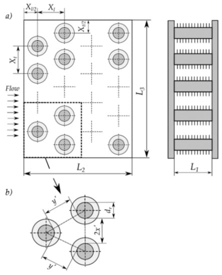
Figure 1.
Finned heat exchanger tube arrangement: (a) airflow through the heat pipes, (b) minimum airflow area (according to [20]).
Minimum airflow area:
where Nf is the number of fins per meter:
in which 2x’ and y’ are given by:
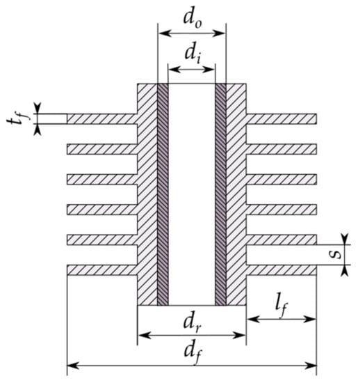
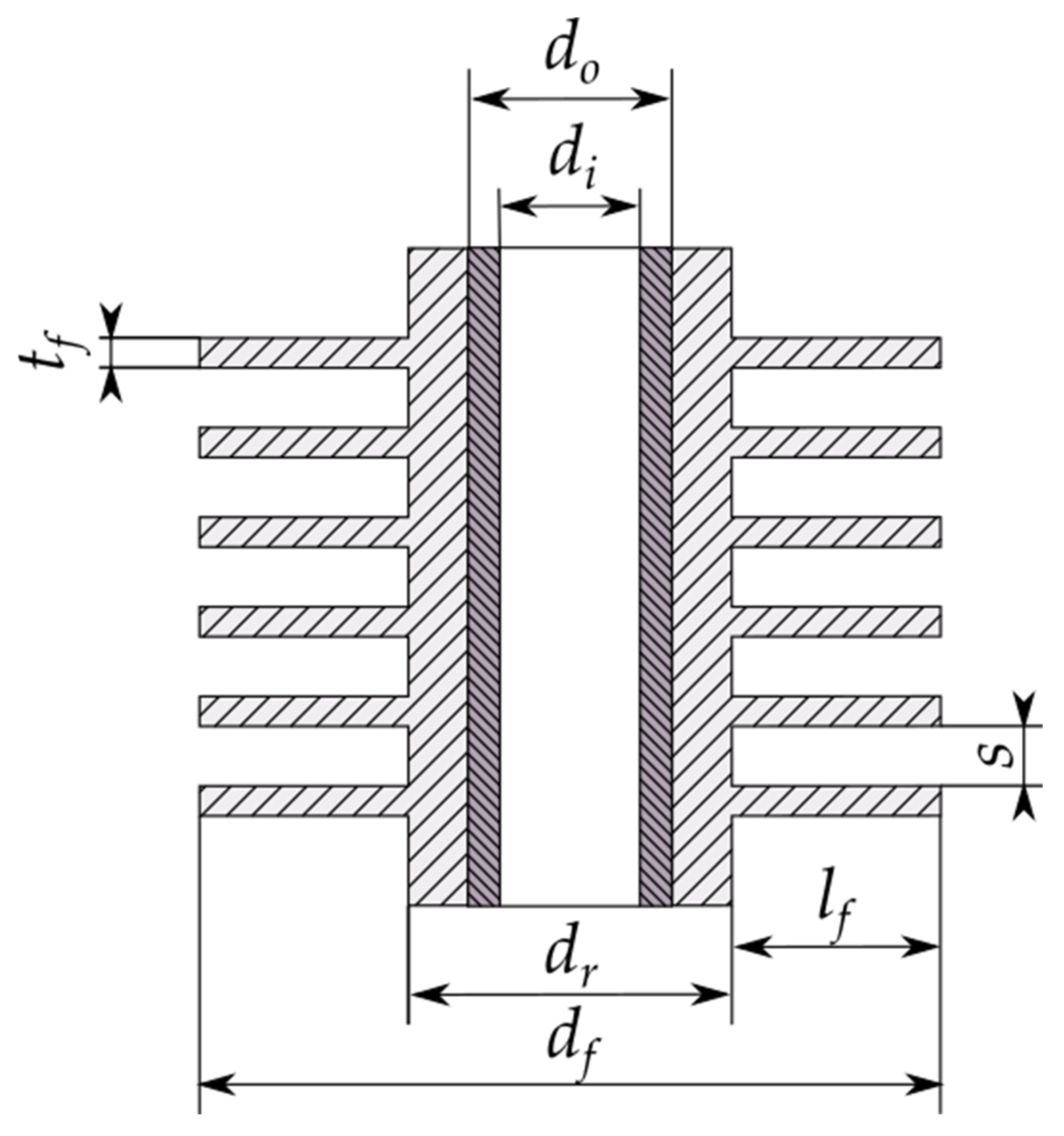
Figure 2.
Geometrical dimensions of finned HP.
For high-fin tube banks, the correlation based on experimental heat transfer data is [21]:
with a standard deviation of 5.1%.
For an equilateral triangular pitch with high-finned tubes, the friction coefficient can be calculated by [21]:
with a standard deviation of 7.8%. This is applicable for the following parameter definitions:
For isosceles triangular layout [22]:
This is applicable for:
where Nt is the number of heat exchanger tube rows.
The pressure drop of airflow through finned tube bundles;
The efficiency of the annular fin (rectangular profile with adiabatic tip) is obtained from correlation [23]:
where ro = df/2, ri = dr/2, I0—modified Bessel function of order 0, I1—modified Bessel function of order 1, K0—modified Bessel function K of order 0, K1—modified Bessel function K of order 1, m coefficient for annular fin:
Finned surface area is obtained by the following equation:
where unfinned area of tube:
finned area of tube:
Overall finned surface efficiency:
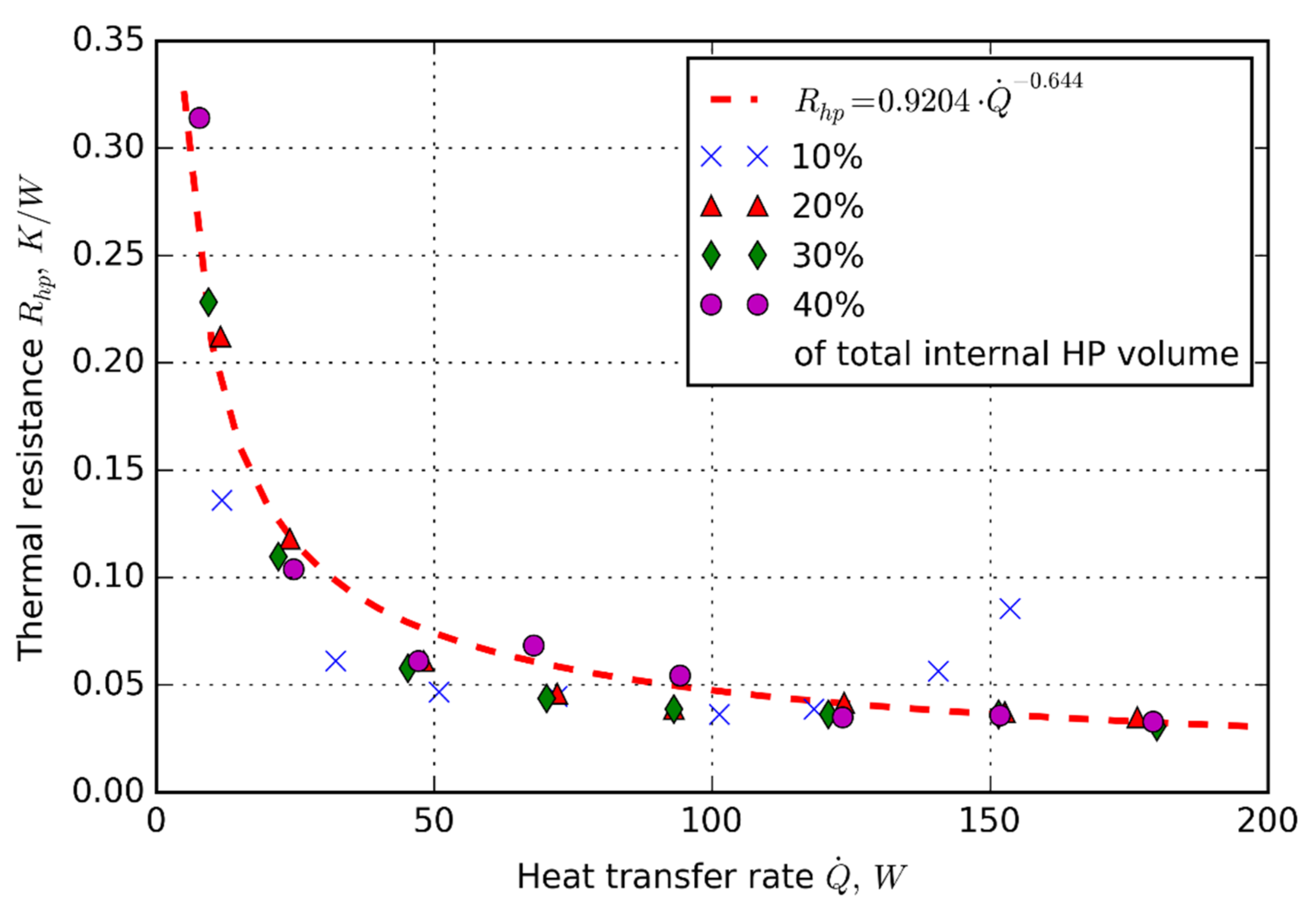
The thermal resistance of the wickless heat pipe is taken from the regression of experimental data from previous authors’ work [22], where the thermal performance of various diameters of wickless HPs were investigated for different working fluids filling ratios. The experiment parameters are summarized in Table 1. Various diameters of HPs were tested to obtain thermal resistance characteristics. On the condenser and evaporator sections of HPs, jacket HEXs were installed. The condenser section HEX was fed with cold water, while through the evaporator section HEX hot water flowed. Because of the low volumetric flow of cooling and heating water, the range of heat fluxes obtained for HPs was nearly identical as predicted in the case of the air-to-air HPHE. The lower convective heat transfer coefficients of the air were compensated for by the area enlargement due to the finned surface (the enlargement factor was around 20). The other aim of the study was to choose the best working fluid of the examined substances. Refrigerant R404A was recognized as the best working fluid (giving the highest thermal throughput) from other tested fluids (R134a, R410A, and R407C). A twenty percent volumetric filling ratio was chosen consecutively as the best of four considered in the study (10%, 20%, 30%, and 40%). Thermal resistance versus heat transfer rate for a 32 mm outer diameter heat pipe is shown in Figure 3. The relative uncertainty of the HPs’ thermal resistance is nearly identical to the relative uncertainty of the heat transfer rate stated in [22] (typically 10–25%). Thermal resistances are nearly identical for filling ratios from 20–40%. They are considerably lower for 10%, although this filling ratio was rejected because of dry-out limit occurrence. Thermal resistance increases sharply for a 10% filling ratio near to the highest heat throughput (near 150 W) because the falling film of the refrigerant was broken, and the dry patches at the evaporator section impeded the heat flow.

Table 1.
Parameters of the experiment [24].
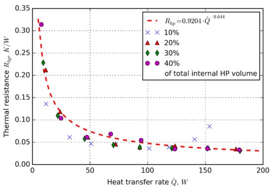
Figure 3.
Thermal resistance of 32 mm outer diameter heat pipe vs. heat transfer rate for different filling ratios [22].
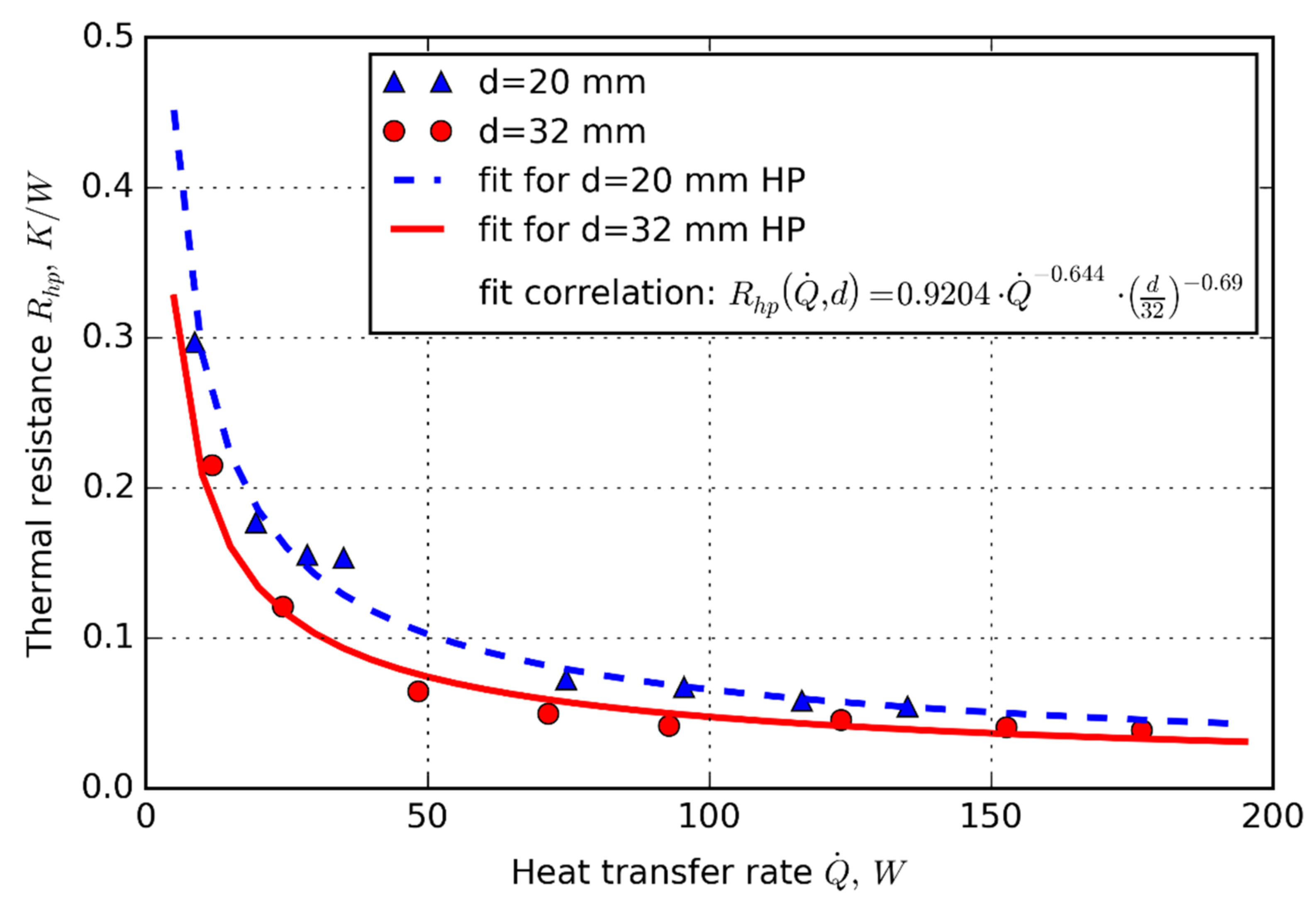
The next lowest filling ratio was considered the best. Even its thermal resistance was comparable with 30 and 40%; lower filling cuts expenses on working fluid and reduces the total weight of HPHE. Experimental data for 20 and 32 mm heat pipes were fitted by a correlation (25) in Figure 4. The correlation takes into account various diameters of HPs. As it can be seen in Figure 4, Equation (25) successfully fits the experimental data [24] for two examined HPs’ outer diameters: 20 and 32 mm.
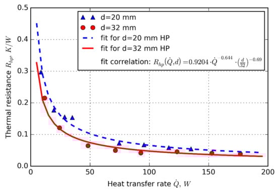
Figure 4.
Thermal resistance vs. heat transfer rate for 20% filling ratio, for d = 20 mm, and d = 32 mm HP. Experimental data were fitted with (25) [23].
Correlation (25) was used to predict the overall thermal resistance of HPs in the computational model:
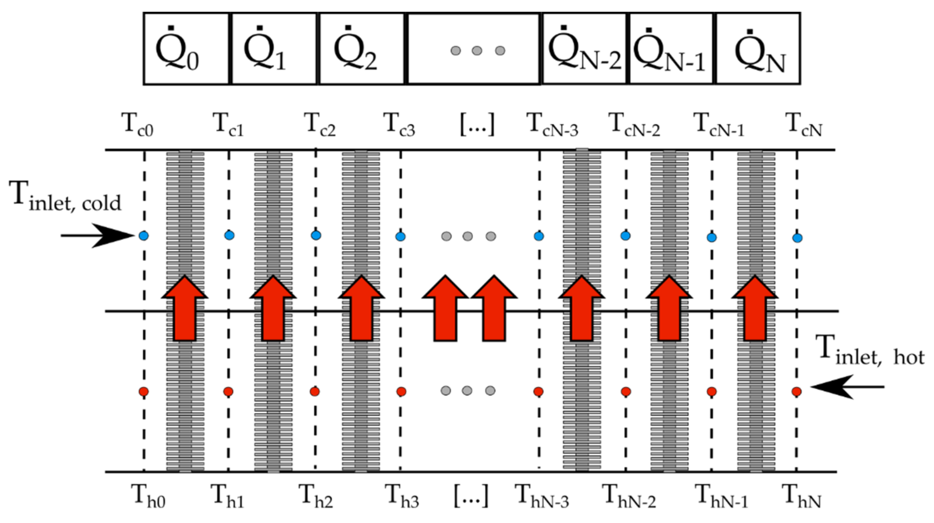
The computational model uses Equations (1)–(25) for the iterative calculation of heat transfer rate, and air streams outlet temperatures. The initial value of the heat transfer rate is guessed and after each iteration, it is updated until the residual becomes lower than 1 W. The iterative technique to solve the non-linear set of equations is the Gauss–Seidel method with an under-relaxation factor of 0.4. This algorithm is used to find a solution (heat transfer rate) for every HPHE row. The HEX is divided into control volumes according to Figure 5. Nodes were at the inlet and outlet planes to each row. Each node represents an unknown temperature, besides the known values at the inlets (blue nodes for cold air temperatures: Tc0–TcN, red nodes for hot air temperatures: Th0–ThN). After all of the temperatures and heat transfer rates were updated, and the maximum residual of all of the temperatures is calculated. If it is not lower than 0.001 °C the temperatures and heat transfer rates are updated again. The iterative technique is also Gauss–Seidel but without the under-relaxation.
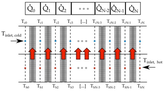
Figure 5.
Scheme of the dividing of HPHE into control volumes.
2.2. Thermal Design Parameters
The design process of HPHE starts with the specification of assumed design parameters which result from HPHE type and its utilization. HPHE will be utilized as an air-to-air recuperator for air conditioning systems. This heat exchanger type implies the following design parameters:
- -
- Working fluid is air at (approximately) atmospheric pressure;
- -
- Effective range of working fluid temperatures is from −20 to 50 °C.
HPHE will be used in very small air conditioning systems (ventilation of up to 160–180 m2 spaces). Both airstreams’ volumetric flow rates are taken as typical for small systems: V = 300 m3/h.
Computational model. The output parameter, which is the main indicator of the efficiency of heat transfer, is HEX temperature effectiveness:
where thi—hot air stream inlet temperature, tho—hot air stream outlet temperature, and tci—cold air stream inlet temperature. A hundred percent recuperation efficiency would occur if the hot stream temperature would drop at the outlet to the level of cold stream inlet temperature.
The goal of optimization is to design HPHE with thermo-hydraulic characteristics (thermal effectiveness, pressure drop) similar to or exceeding most of the existing HPHE reported earlier in the literature review. Comparative parameters are:
- -
- Pressure drop: 40 Pa (not greater than 200 Pa);
- -
- Thermal efficiency: 60%.
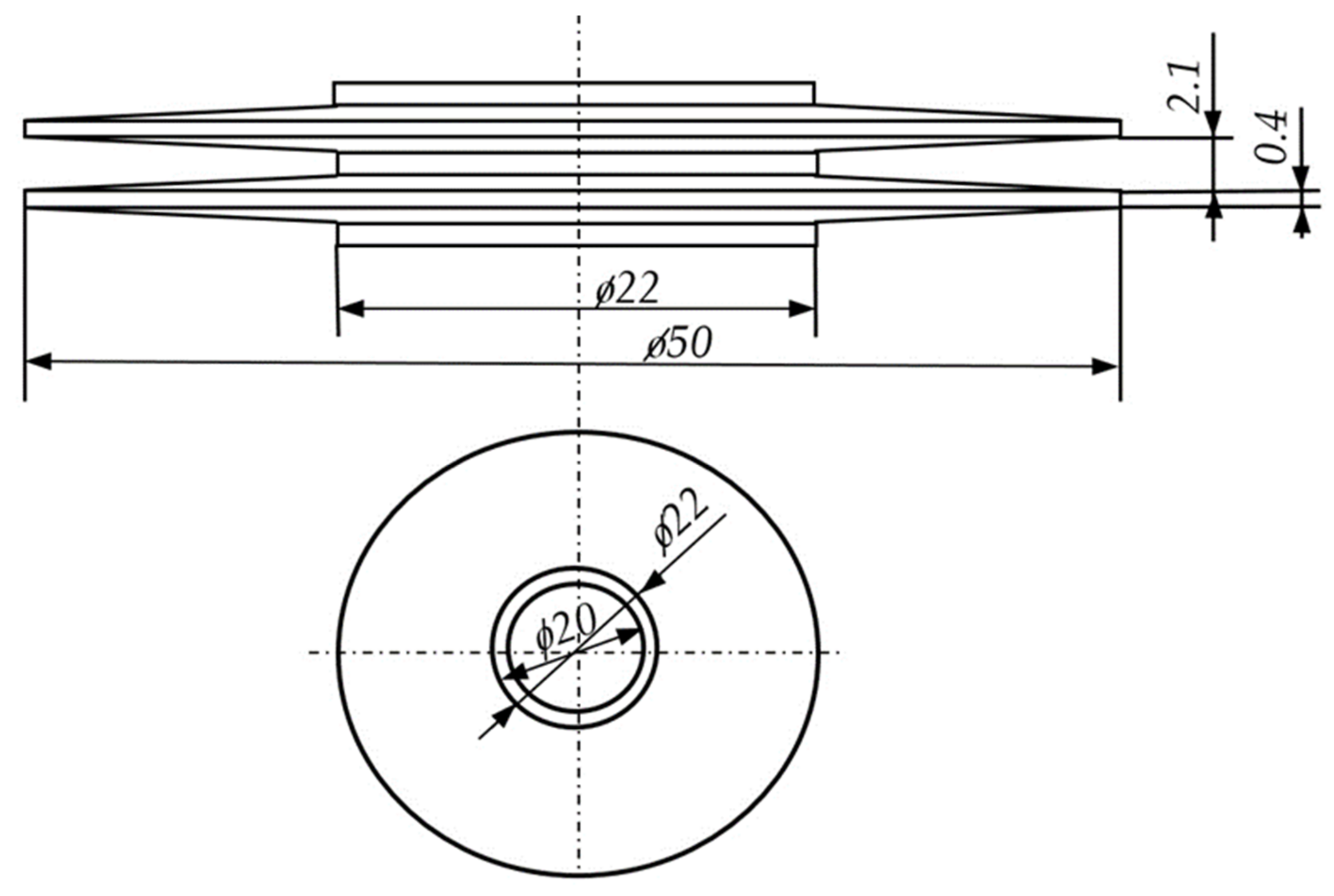
The geometry of the finned tube was chosen to ensure the ease of HPHE prototype manufacture. It was selected from the bimetallic high-finned tubes manufacturer catalog—CEMAL company [24]. Heat exchanger channel height was L1 = 0.245 m (a consequence of finned heat pipe geometry), and width L3 = 0.245 m was a result of the assumption of a square channel. Geometrical parameters of the finned aluminum tube applied on the standard copper tube: ø 22 × 1 mm are given in Table 2 and presented in Figure 6. Fins were cold-rolled on the outer aluminum tube.
Table 2.
Geometrical parameters for the high-finned tube.
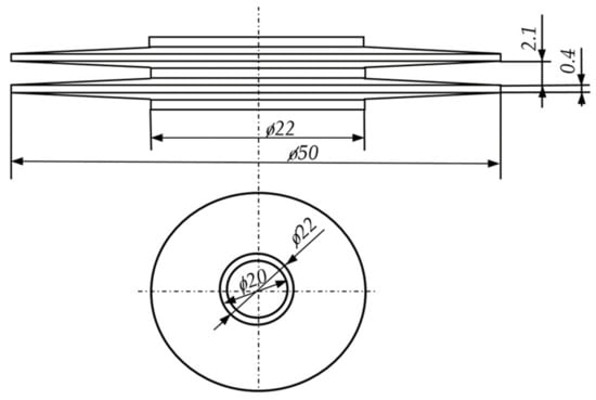
Figure 6.
Finned surface heat pipe heat exchanger dimensions.
2.3. Parametric Optimization of HPHE
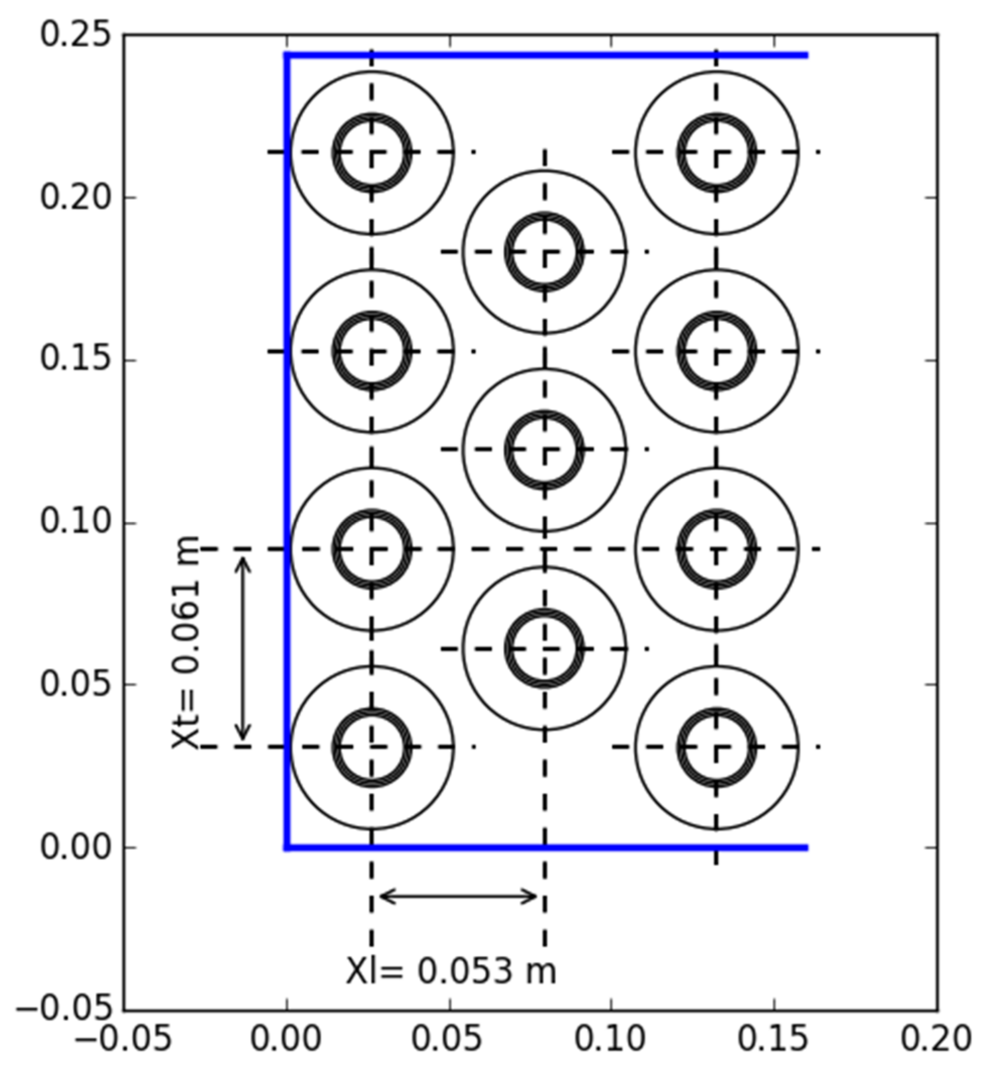
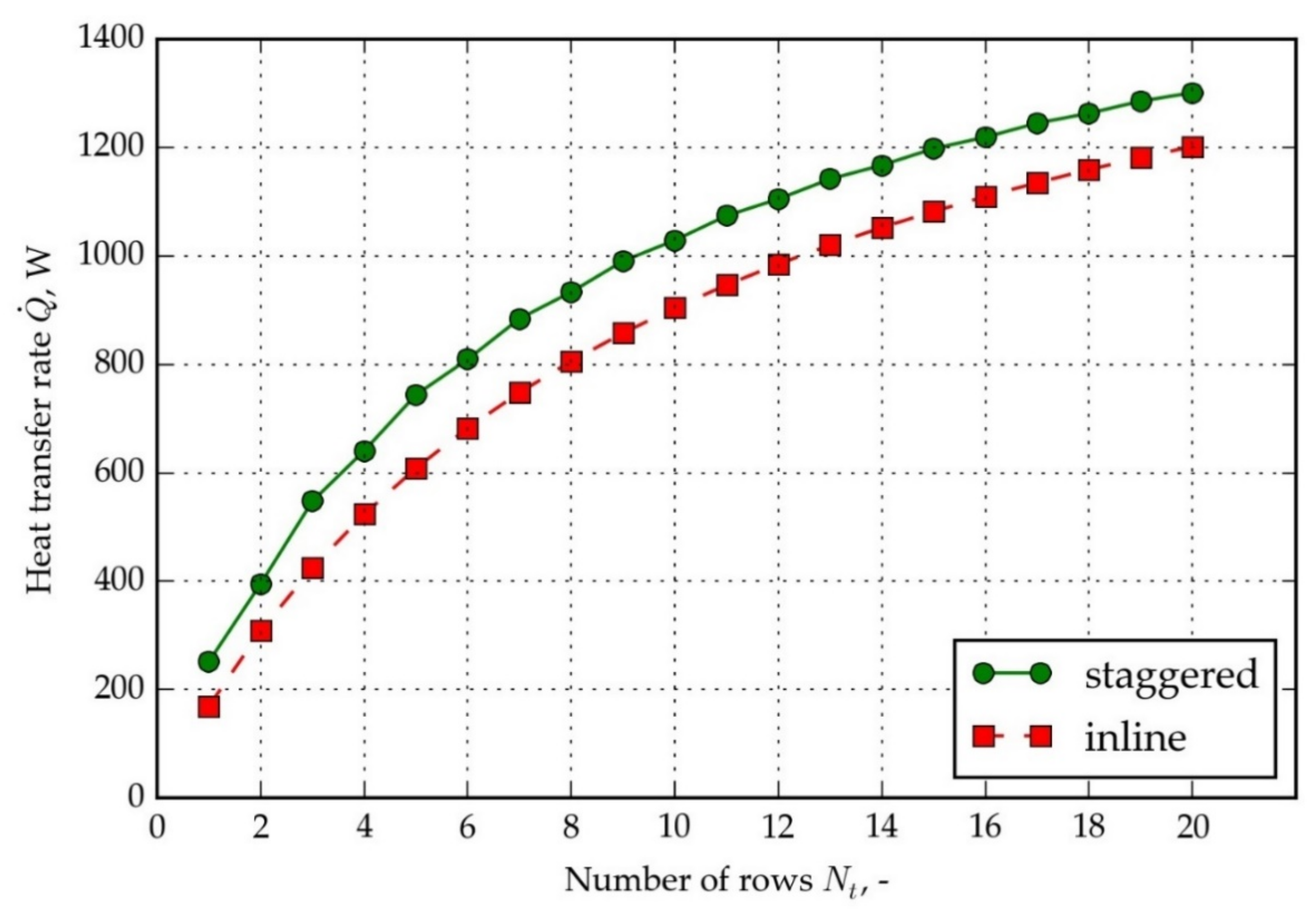
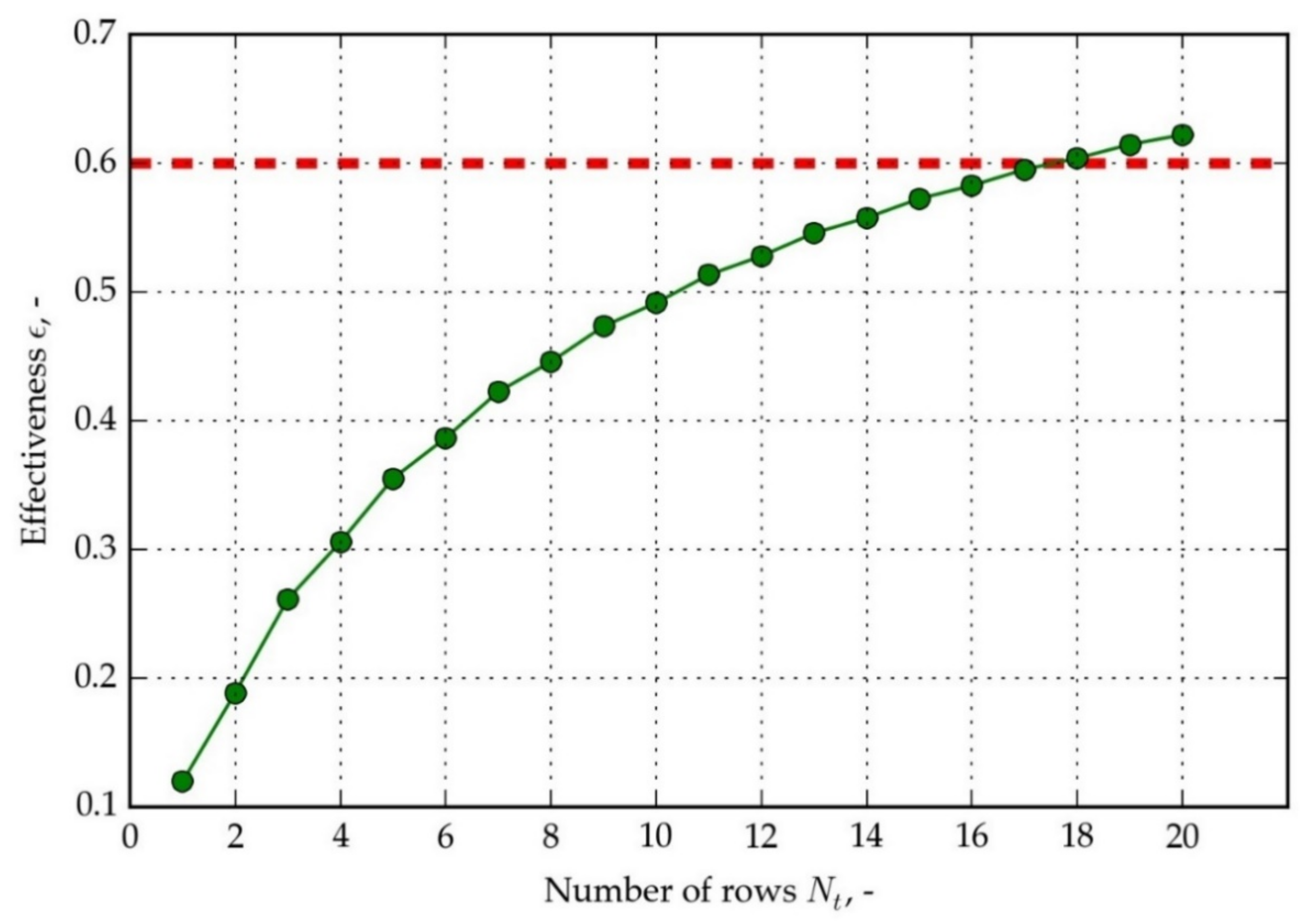
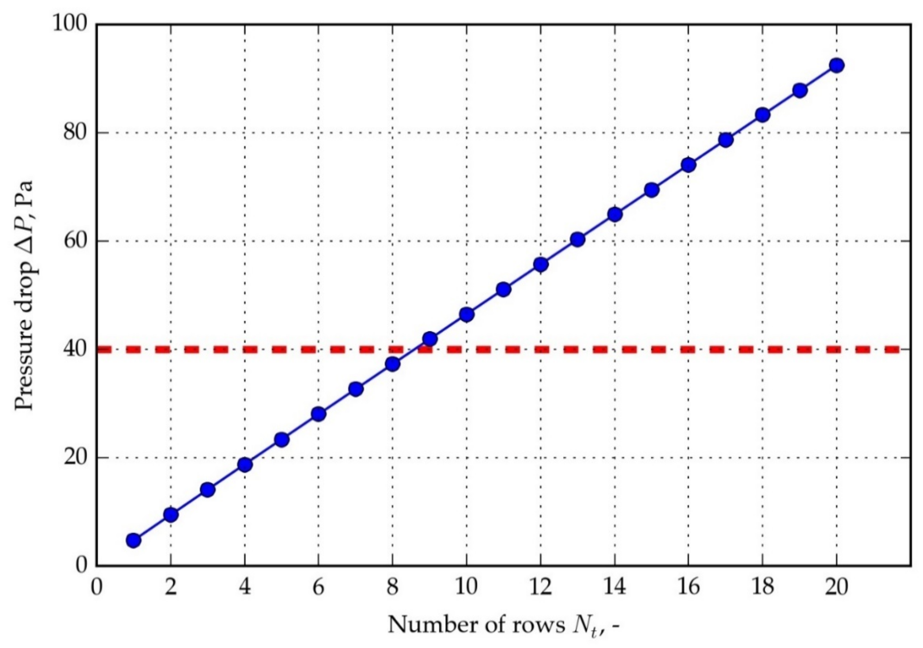
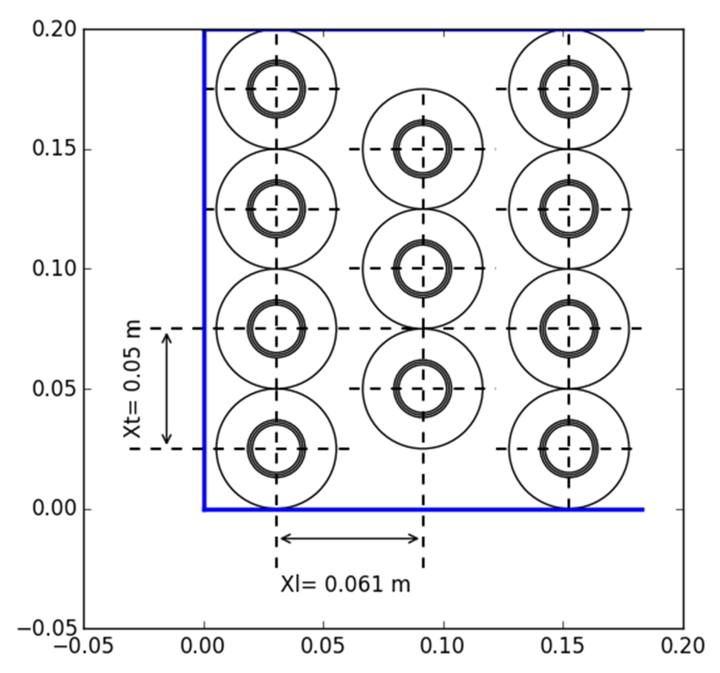
The initial arrangement of finned heat pipes is shown in Figure 7 (three first rows). It is a start positioning for the further thermal and flow analysis carried out with the use of the computational model. This arrangement is considered for the first set of plots: Figure 8, Figure 9 and Figure 10. Volumetric flow rates for hot and cold airstreams are held constant (300 m3/h). Inlet cold air temperature is kept at 10 °C and hot air inlet temperature at 30 °C. The counterflow arrangement was chosen as it produces a higher mean temperature difference between streams than parallel flow. A staggered HPs arrangement was also selected over the inline as it ensures better mixing and temperature uniformity of air streams. Initially, the isosceles layout was assumed due to a minimal pressure drop [20]. Figure 8 shows the heat transfer rate for inline and staggered finned HPs arrangement as a function of the number of HPHE rows. It is a validation of the correctness of the computational model calculations. As expected in the whole, considered range of the number of rows, the staggered arrangement produces a higher heat transfer rate than inline. As the number of rows increases, thermal effectiveness grows non-linearly (Figure 9)—the shape of the function is similar as in the case of heat transfer rate. The previously stated goal is 60% effectiveness (red horizontal line), and it corresponds to a 17-rows HPHE. Because of thermal calculations uncertainty, 20 rows were chosen (three extra rows) to obtain the assumed effectiveness. Pressure drop increases linearly with the number of rows and exceeds 40 Pa at approximately nine rows (Figure 10). For 20 rows HPHE, ∆P of 100 Pa is not exceeded, which makes that acceptable value for small air conditioning systems (it can be handled by a typical air duct fan). Further increase in effectiveness by adding more rows (more than 20) is not viable, because the addition of two rows produces approximately 10 Pa extra pressure drop (which is 10% relative increase) while only 2–3% raise of effectiveness. It supports 20 rows as the final choice, taking into account that a pressure drop increases linearly, while the effectiveness slope becomes less steep for increasing row number (adding more rows becomes even less viable in terms of effectiveness vs. ∆P change as row number increases).
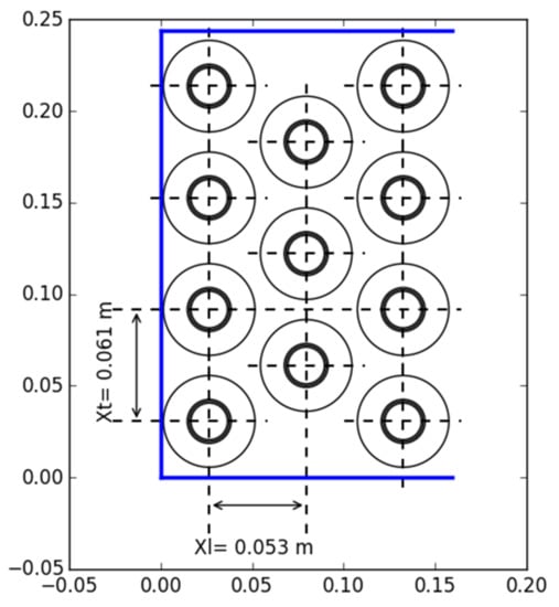
Figure 7.
The initial arrangement of the HPs in HPHE (staggered).

Figure 8.
Heat transfer rate for inline vs. staggered heat pipe arrangement, for inlet cold air temperature 10 °C and hot air inlet temperature 30 °C.

Figure 9.
Thermal effectiveness of HPHE as a function of number of rows, for inlet cold air temperature 10 °C and hot air inlet temperature 30 °C.
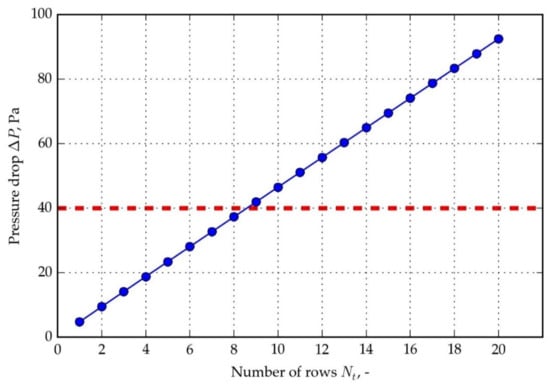
Figure 10.
Pressure drop for HPHE vs. number of rows, for inlet cold air temperature 10 °C and hot air inlet temperature 30 °C.
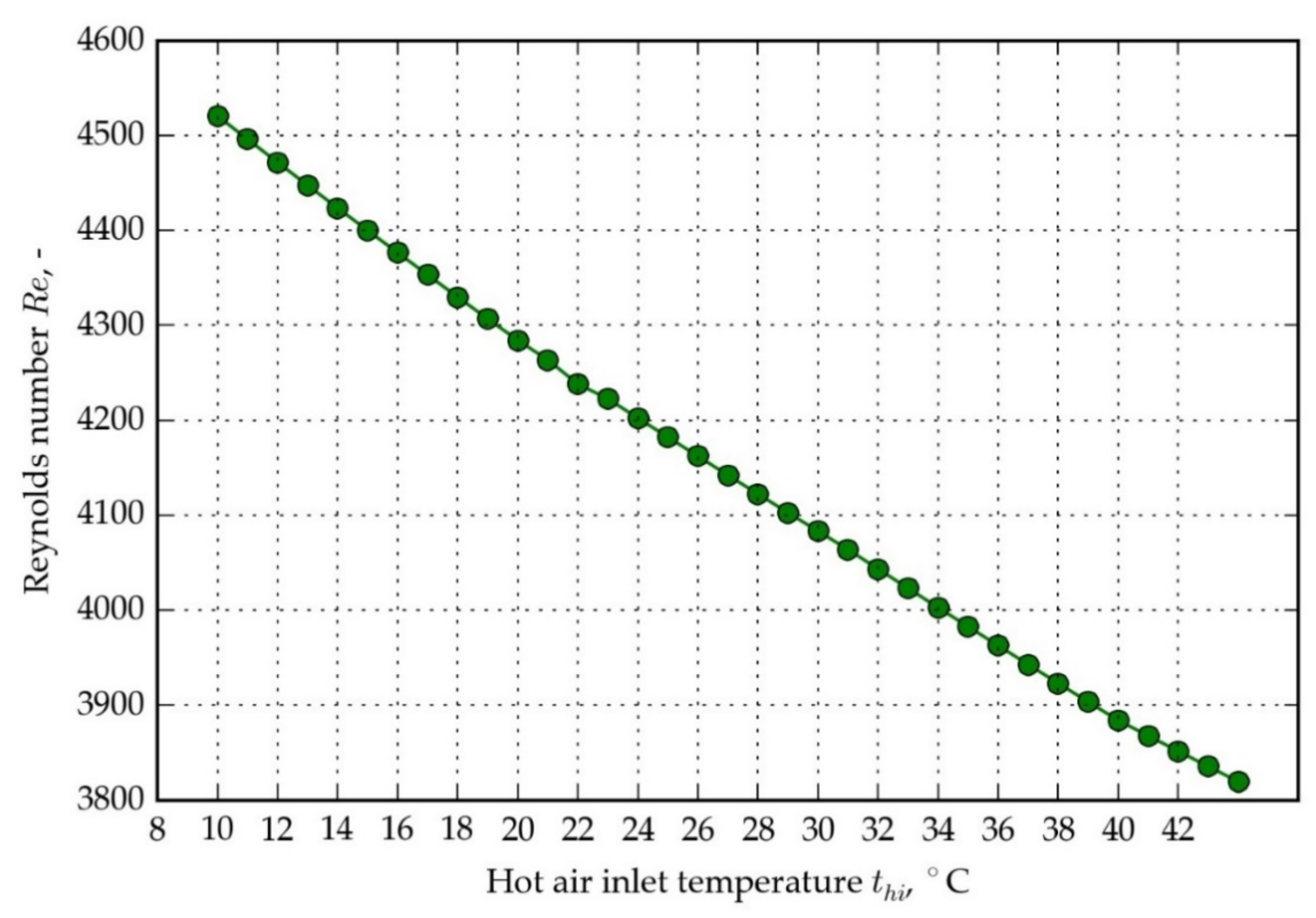
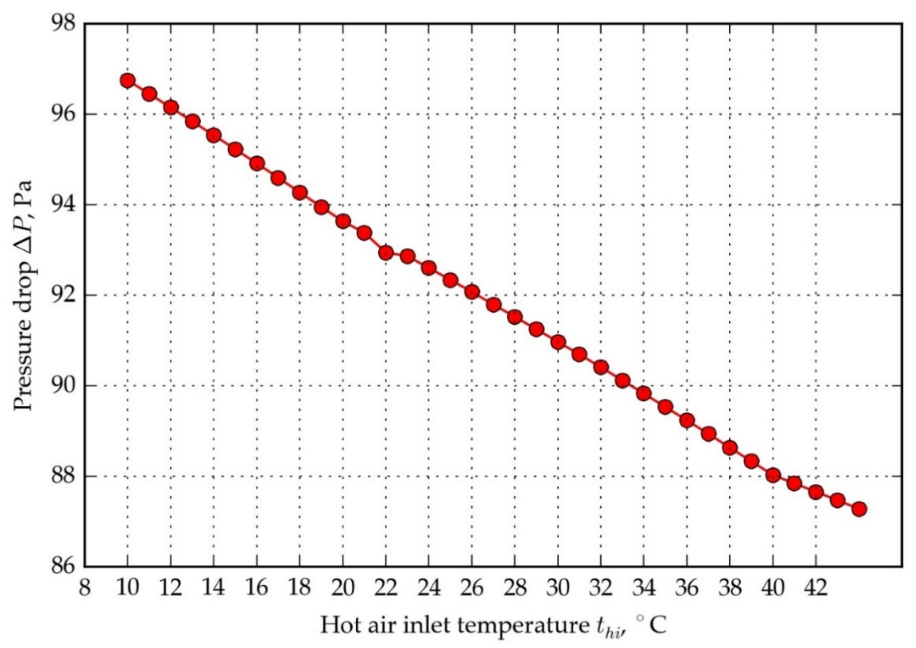
The dependence of parameters on hot air inlet temperature is shown in Figure 11, Figure 12 and Figure 13. All computations for the plots were made with the assumption of 20 HPs rows and 0 °C cold air stream inlet temperature. Figure 11 shows the dependence of the Reynolds number, which is decreasing for increasing hot air inlet temperature. It is an effect of an increase in air kinematic viscosity with temperature. There is approximately a 15% Reynolds number decrease relative to the value for the lowest considered temperature: 8 °C. Figure 12 presents the pressure drop as a function of the hot air inlet temperature. The pressure drop decreases linearly by 10% for the assumed temperature range—it is caused mainly by a decrease in air density with temperature. The combined effect of air thermophysical properties changes with temperature (variation with pressure is negligible) and mean temperature rise impacts HPHE effectiveness, yet very weakly for hot air temperatures greater than 30 °C (Figure 13). The relative change from 30 to 42 °C is just a fraction of a percent. The above analysis shows that the assumption of approximately 60% effectiveness is valid for a broad range of temperatures for 20 rows of HPHE. There is a potential benefit in reducing a pressure drop for higher temperatures, although it is calculated for a constant volumetric flow of air, which could decrease in a real situation, where a fan is inducing the flow. The working point of a fan can change for lower air density and flow conditions could vary.

Figure 11.
Reynolds number vs. hot air inlet temperature, for cold stream inlet temperature 0 °C and 20 HPs rows.

Figure 12.
Pressure drop vs. hot air inlet temperature, for cold stream inlet temperature 0 °C and 20 HPs rows.
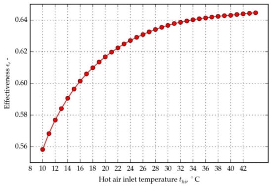
Figure 13.
Effectiveness vs. hot air inlet temperature, for cold stream inlet temperature 0 °C and 20 HPs rows.
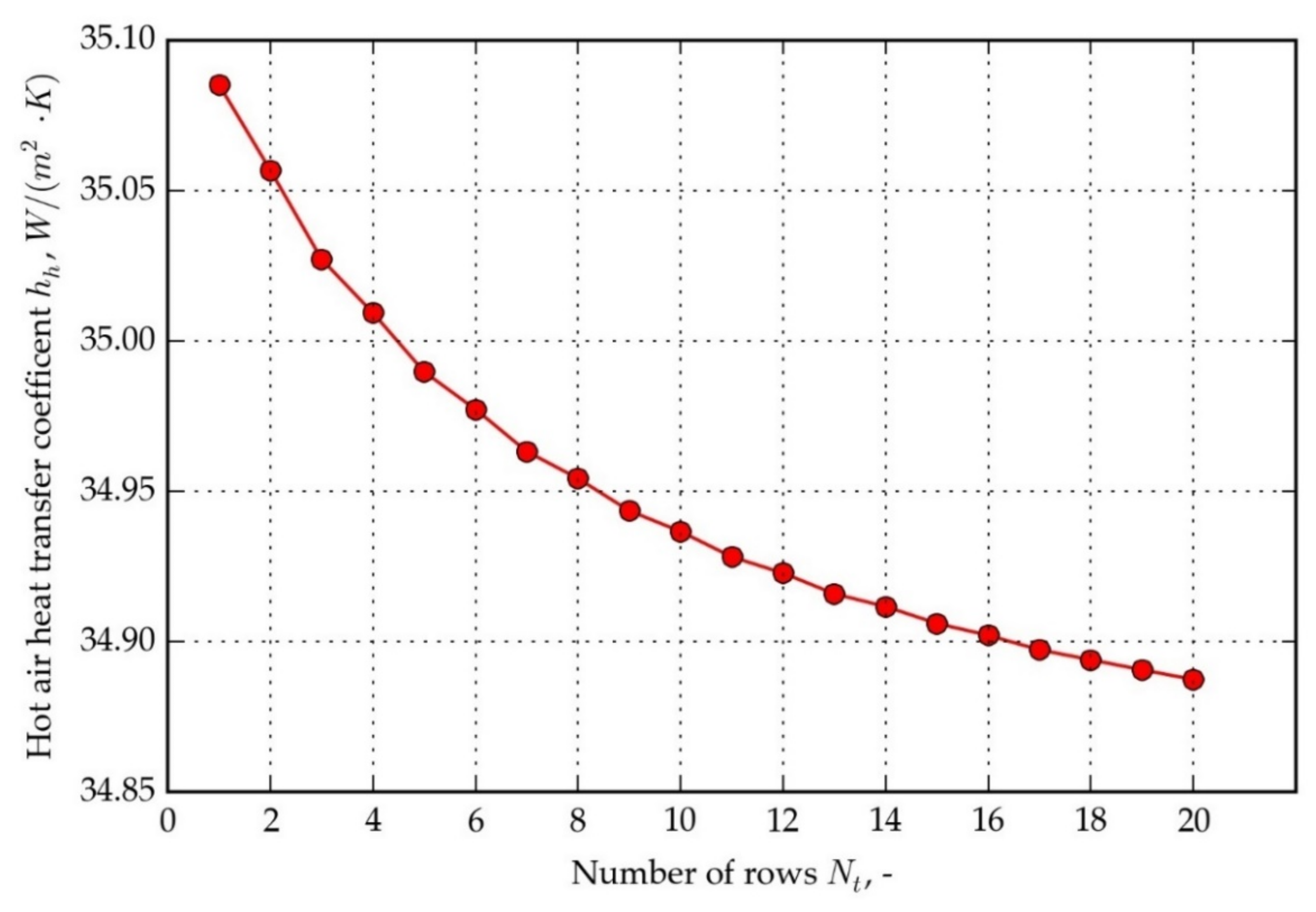
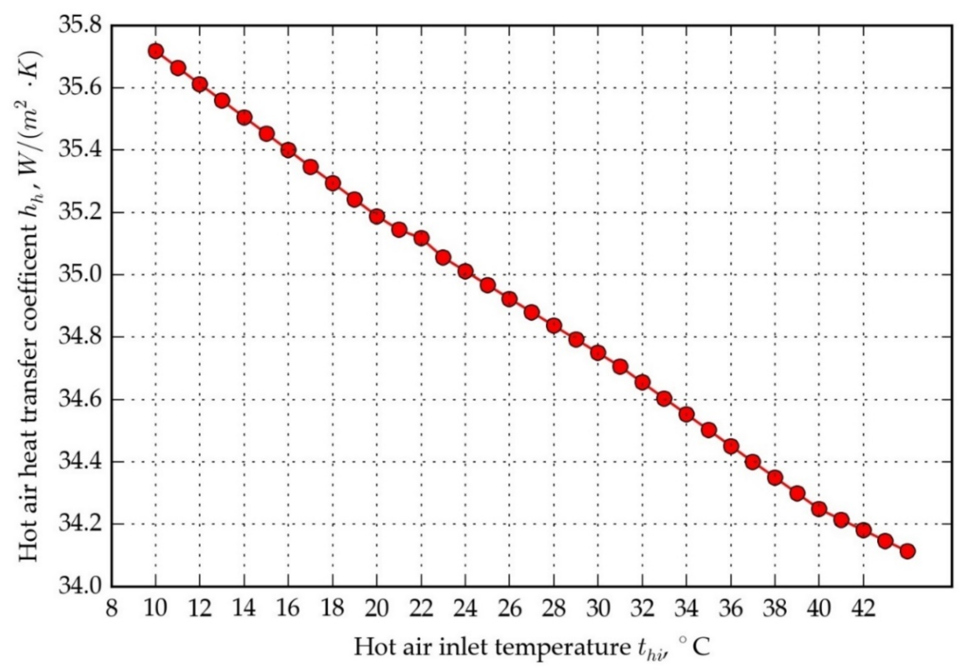
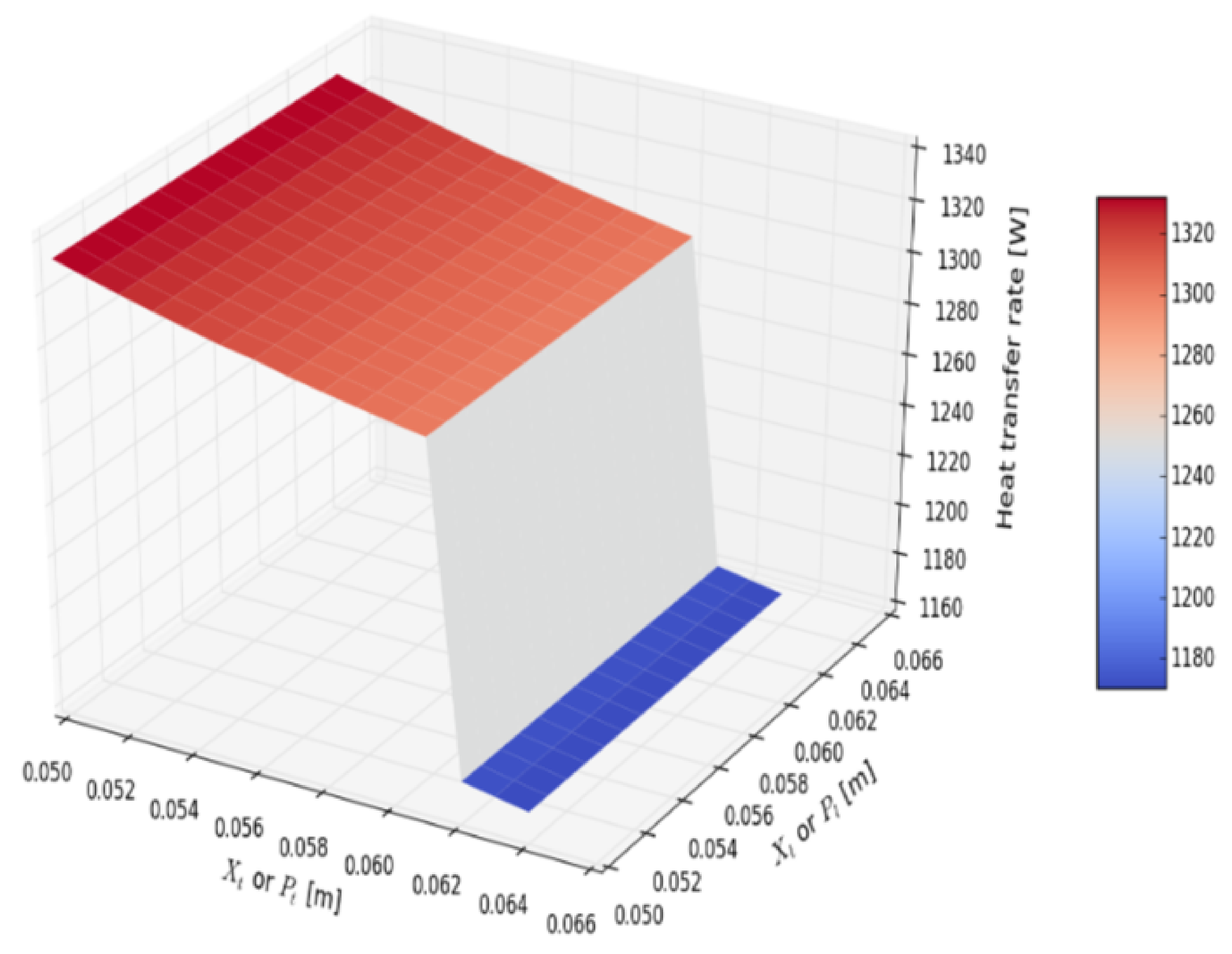
Figure 14 shows hot air heat transfer coefficient dependence on the number of rows (inlet hot air temperature: 30 °C, inlet cold air temperature: 10 °C). The computational model allows very small dependency of the heat transfer coefficient as equation (15) is valid for the number of rows greater than six; therefore, the calculated heat transfer coefficients for a smaller number of rows are uncertain. This inaccuracy, however, is not very important, as the practical number of rows which produces reasonable HPHE efficiency (ε > 50%) is greater than 10. The dependence of the hot air heat transfer coefficient on the hot air inlet temperature, for cold air inlet temperature 0 °C, is shown in Figure 15. For the broad range of temperatures, heat transfer coefficient changes only slightly—it drops by 5%. This proves the stability of the working point of HPHE under various temperature conditions. Three-dimensional graphs are introduced for defining the optimal spacing between the center of the tubes—longitudinal and traversal in the respect to the airflow direction. The subsequent analysis was carried out with an assumption of constant hot and cold air inlet temperatures (10 and 30 °C). Figure 16 presents the exchanged heat transfer rate as a function of traversal and longitudinal spacings. Heat transfer rate changes stepwise at Xt = 0.062 m because below that spacing it is possible to add one extra HP in the row. Further decrease in traversal distance results in weak growth. At minimal traversal spacing Xt = 0.05 m (contact of finned HPs), heat transfer rate attains the maximal value. Longitudinal spacing does not affect the heat transfer rate. HPHE effectiveness, shown in Figure 17, exhibits similar behavior to heat transfer rate, with the peak value of 64% for minimal traversal spacing. The pressure drop rises more sharply with the decrease in Xt than with the reduction in Xl. As longitudinal spacing does not affect heat transfer significantly, moving away HPs in the longitudinal direction is advised, yet excessive spacing could cause an unacceptable increase in the total length of HPHE. The peak of a pressure drop is noted for minimal spacings (approx. 160 Pa).

Figure 14.
Hot air heat transfer coefficient vs. the number of rows, for hot air inlet temperature 30 °C and cold air inlet temperature 10 °C.

Figure 15.
Hot air heat transfer coefficient vs. hot air inlet temperature, for cold air inlet temperature 0 °C.

Figure 16.
Heat transfer rate vs. traversal and longitudinal spacing of the tubes.
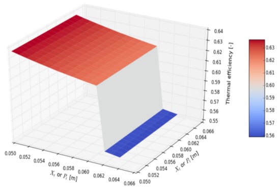
Figure 17.
Thermal efficiency vs. traversal and longitudinal spacing of the tubes.
The hot air heat transfer coefficient grows by 20% with traversal spacing reduction (Figure 18). Enhancement by altering the Xl is negligible. Figure 19 presents the dependence of HPHE effectiveness on Xt and hot air inlet temperature. A maximal value of 66% is attained for minimal Xt and the maximal temperature difference between hot and cold airstreams. As expected for higher temperature differences, HPHE performs better.
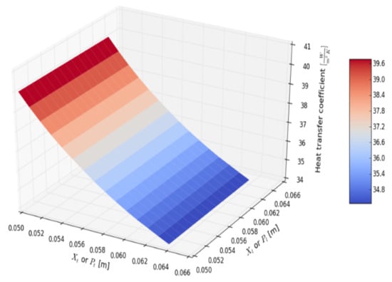
Figure 18.
Heat transfer coefficient vs. traversal and longitudinal spacing of the pipes.
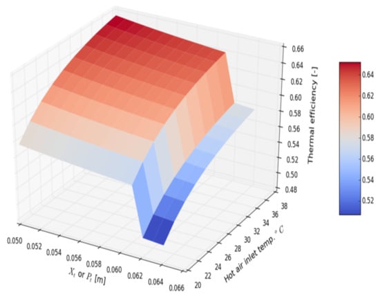
Figure 19.
Thermal efficiency vs. traversal spacing of the pipes and hot air inlet temperature.
3. Validation of Computational Model by the Experiment
The prototype of HPHE was manufactured for the validation of the computational model. The HPHE tests were carried out in three successive measurement series. Each series was characterized by different values of air volumetric flows in the ducts caused by the change in rotational speed of the radial fans. The rotational speed of the fans was varied by fan motor speed controllers (based on TRIAC’s electronic circuits). The measurement series consisted of three tests, during which the volumetric flow rates of the fluid flowing in the channels were kept steady.
The first measurement series was carried out at average volumetric flows of approx. 530 m3/h (hot air duct) and approx. 400 m3/h (cold air), respectively.
The second measurement series was carried out with average volumetric flows of approx. 520 m3/h (hot air duct) and approx. 460 m3/h (cold air), respectively. This series is distinguished by a high-volume flow rate in the hot air duct.
The third measurement series was carried out at average volume flows of approximately 380 m3/h (hot air duct) and 370 m3/h (cold air), respectively. This series was characterized by the lowest average volumetric flows in the air channels. The range of airflows corresponds to average velocities: 1.7–2.5 m/s, which is typical for small air-conditioning ducted systems (for systems with capacities < 1000 m3/h, 3 m/s velocity is considered maximal, to avoid high pressure drops). HEX studies were conducted at the experimental rig shown in Figure 20.
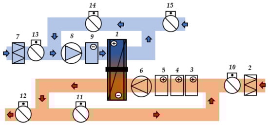
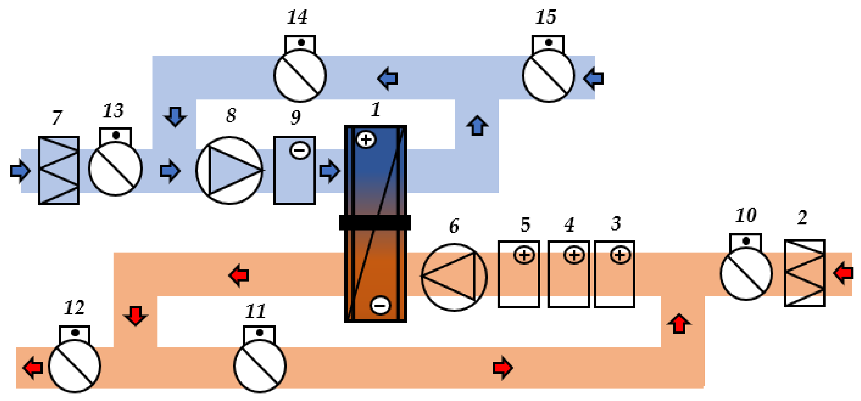
Figure 20.
Diagram of the HPHE test rig: 1—HPHE; 2, 7—air filters; 3–5—electric preliminary heaters; 6, 8—air fans; 9—air cooler; 10–15—manual dampers.
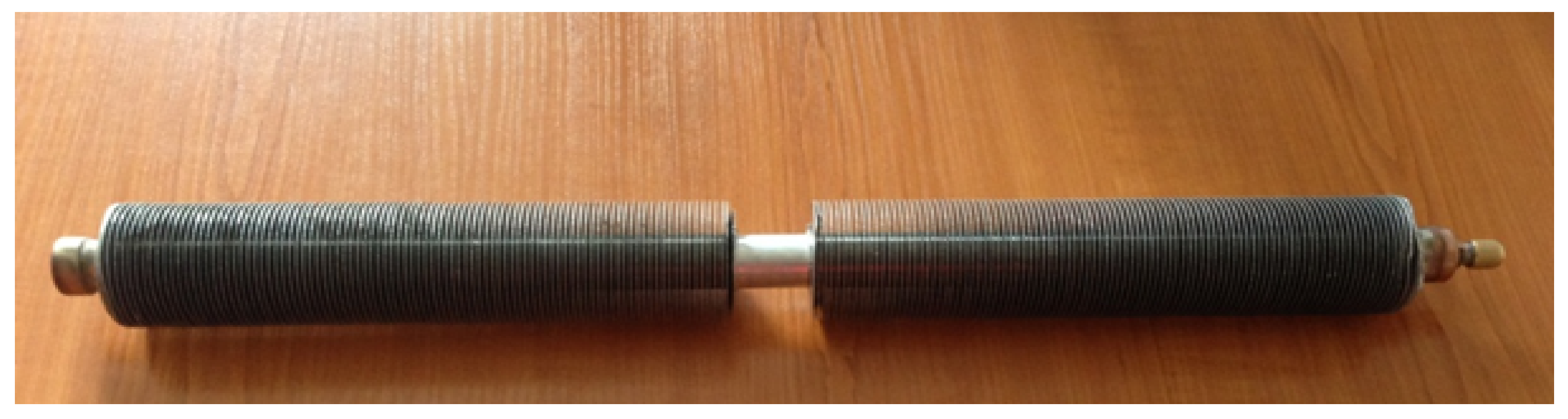
The subject of the test is a HEX (1) made of finned SHP (Figure 21) for the recovery of heat from exhaust air.
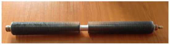
Figure 21.
Photo of the finned heat pipe.
Two air streams (hot—exhaust and cold—fresh air) pass through the HEX. The airflow arrangement is countercurrent. The HEX is made up of 32 HPs in a staggered arrangement. Each of the HP’s is filled with R404A refrigerant. Based on previous research [22] the optimal amount of refrigerant in HP has been determined as 20% of its volume. Air flows through steel air ducts with a diameter of d = 0.2 m, while in the part adjacent to HPHE they transform into ducts with a rectangular flow area: 0.24 m × 0.25 m. Streams of the exhaust (hot) and fresh (cold) air flow in closed circuits. Airflow in the ducts is forced, utilizing fans (6, 8). There is one fan for exhaust and one for fresh air. The speeds of both fans are individually regulated. The air parameters are regulated by a cooler (9) and heaters (3–5). Cooler is an element of a split refrigeration system (refrigerant R404A). The air-cooled condenser, which is expelling the heat absorbed from an air stream, is placed outside the building. The cooling capacity is regulated by manually adjusting the automatic expansion valve opening, which is metering a refrigerant flow to the cooler. Heaters are simple electric air duct heaters. There is a temperature probe upstream of every heater for the feedback to the automation system controlling the power output for obtaining the pre-set temperature. Air is drawn in through filters (2, 7) and the flow direction is controlled by mechanical dampers. The experimental rig arrangement allows for cooling only the top channel of HPHE and heating the bottom channel (Figure 19).
The air system can operate in both closed and open circuit (drawing or releasing air to outside). The experimental tests were carried out in conditions where supply and fresh air flowed in closed circuits without contact with the external air. Both HPHE flow channels were divided into 27 equal areas. In the centers of these areas, velocity and temperature measurements were taken. In each of the measurement planes, the average velocity and temperature were calculated based on 27 measurements. The temperature and velocity measurements were performed utilizing the “climate meter” probe LB-580 [25], which has the functions of a thermal anemometer, thermometer (Pt1000), and capacitive hygrometer. The mass flow rate was calculated from the average value of the velocity at the measurement planes. In each of the airflow ducts (fresh and exhaust air) there were two measurement planes—directly upstream and downstream of the HPHE. The differences between the average velocities of a single airstream did not exceed 5%. The average relative humidity of air was also checked at the inlet and outlet of HPHE, but in any of the cases no change was recorded, so no water vapor condensation occurred on the heat exchange surfaces.
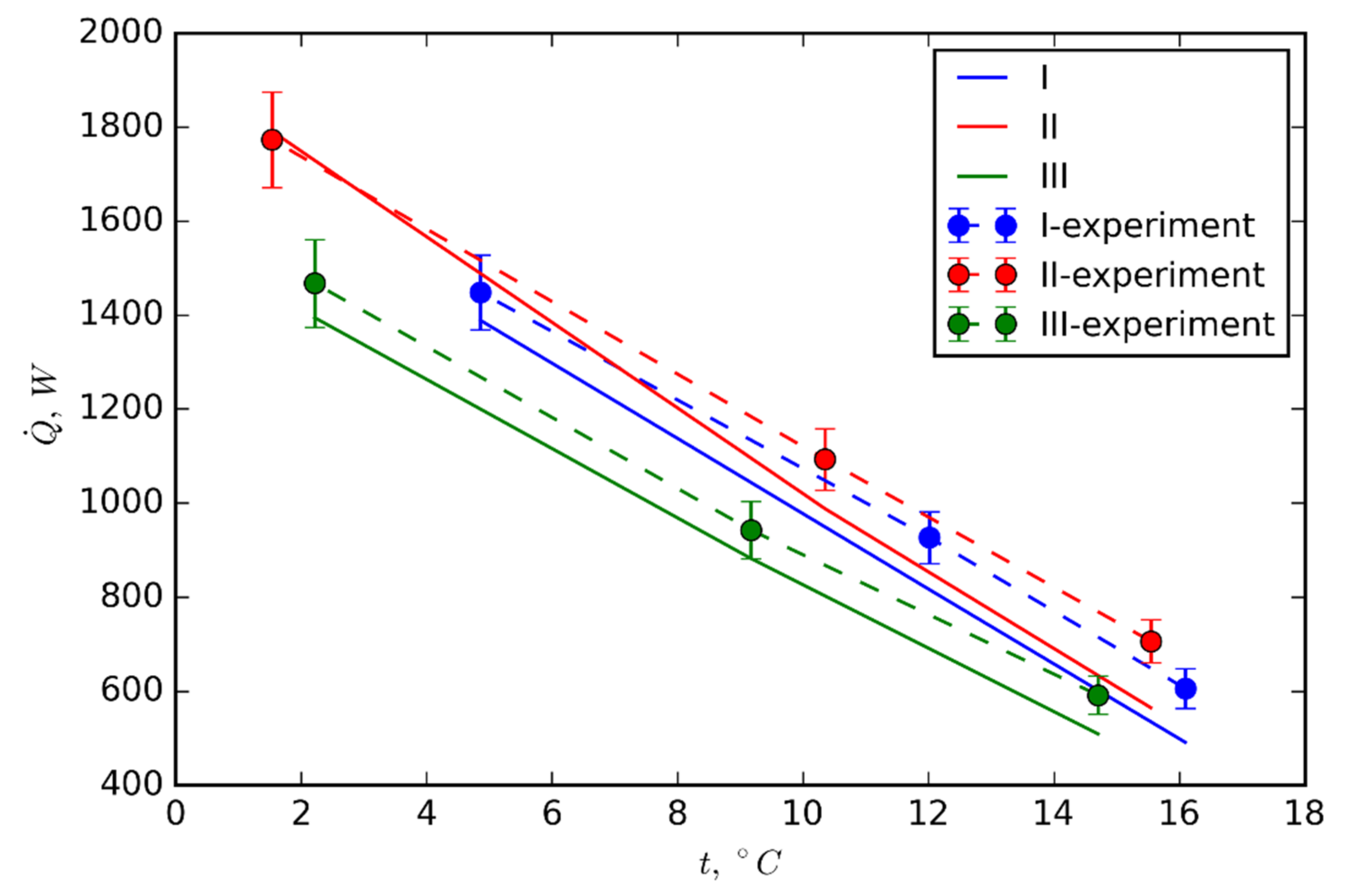
The graph shown in Figure 22 specifies the values of the average heat transfer rates depending on the set temperature of the fresh (cold) air at the HPHE inlet for three measuring ranges, differing in the average air volumetric flow rates in the ducts. The experimental values were shown with error bars and computed values from the numerical model. The temperature of the fresh air at the inlet to the HPHE in the condenser section changed according to Figure 3 and in the evaporator section, it was kept at 24 °C. The charts were made for the air flows shown in Table 3.
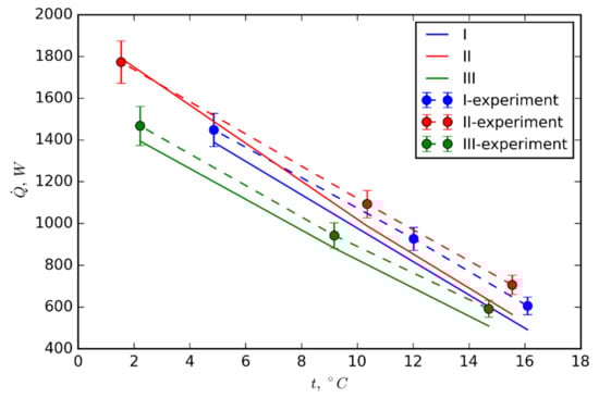
Figure 22.
Average HPHE heat transfer rates from model and experimental for varying volumetric airflow rates.
Table 3.
Exhaust and fresh air flows.
The characteristics presented in Figure 22 show that with the increase in the temperature at the inlet of the fresh air, the heat transfer rates became lower. The decrease in the average air volume flows in individual measurement series is accompanied by a decrease in the average heat transfer rates. The highest average experimental heat transfer rate, 1773 W, was obtained for the second case, for which the average temperature measurement of the fresh air at the heat exchanger inlet was equal to 1.5 °C. The lowest average heat flux of 592 W was obtained for the third case and the fresh air temperature of 14.70 °C. There is a good agreement between experimental heat transfer rates and those obtained from the model described in the following section—the average difference between measured and computed values is approximately 10%. In the high heat transfer rates region, the model output is within the estimated measurement uncertainty. Relative uncertainty is in the range of 5–8%. The model is more differing from the experimental data for the smaller heat fluxes. As can be seen in Figure 22, as fresh air inlet temperature increases, the measurement, and numerical curves diverge. The highest relative difference is 20%, the lowest is 1%. The reason for the higher discrepancy for lower heat fluxes can be the higher uncertainty of the heat pipe thermal resistance for low throughputs. The same argument could be made for the airside convective heat transfer correlation.
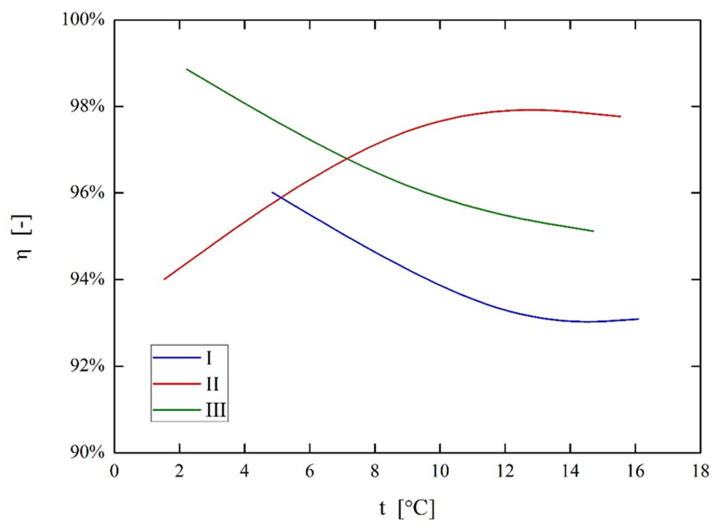
Figure 23 shows the values of the experimental HEX efficiency η defined as the ratio of the heat transfer rate absorbed by the fresh air to the value of the heat transfer rate released by the exhaust air. These values depend on the average inlet temperature of the fresh air. The graph shows the characteristics for three cases, characterized by different average fluid volumetric flow rates.
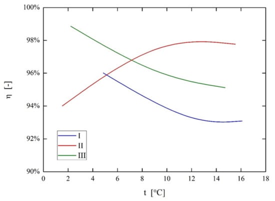
Figure 23.
HEX efficiency η versus the fresh air temperature at the inlet to HEX for different volumetric flow rates.
Based on the above diagram, it can be concluded that the efficiency of the HEX η decreases in most cases with increasing temperature of the fresh air at the inlet. The exception is the second case, for which the average volume flows were 520 m3/h (the exhaust air duct) and 460 m3/h (the fresh air duct). At a lower average temperature (1.54 °C), a lower efficiency (94%) was obtained than for similar measurements at higher temperatures (97.8%). The lowest efficiency (93%) was obtained for the temperature of 16.09 °C, which leads to the conclusion that it is worth ensuring that the HEX works with air at possibly the lowest temperatures. The highest efficiency (98.9%) was obtained for the third measurement of the third series (2.22 °C). In the entire tested range, the efficiency of the HEX was in the range of approx. 93–98%.
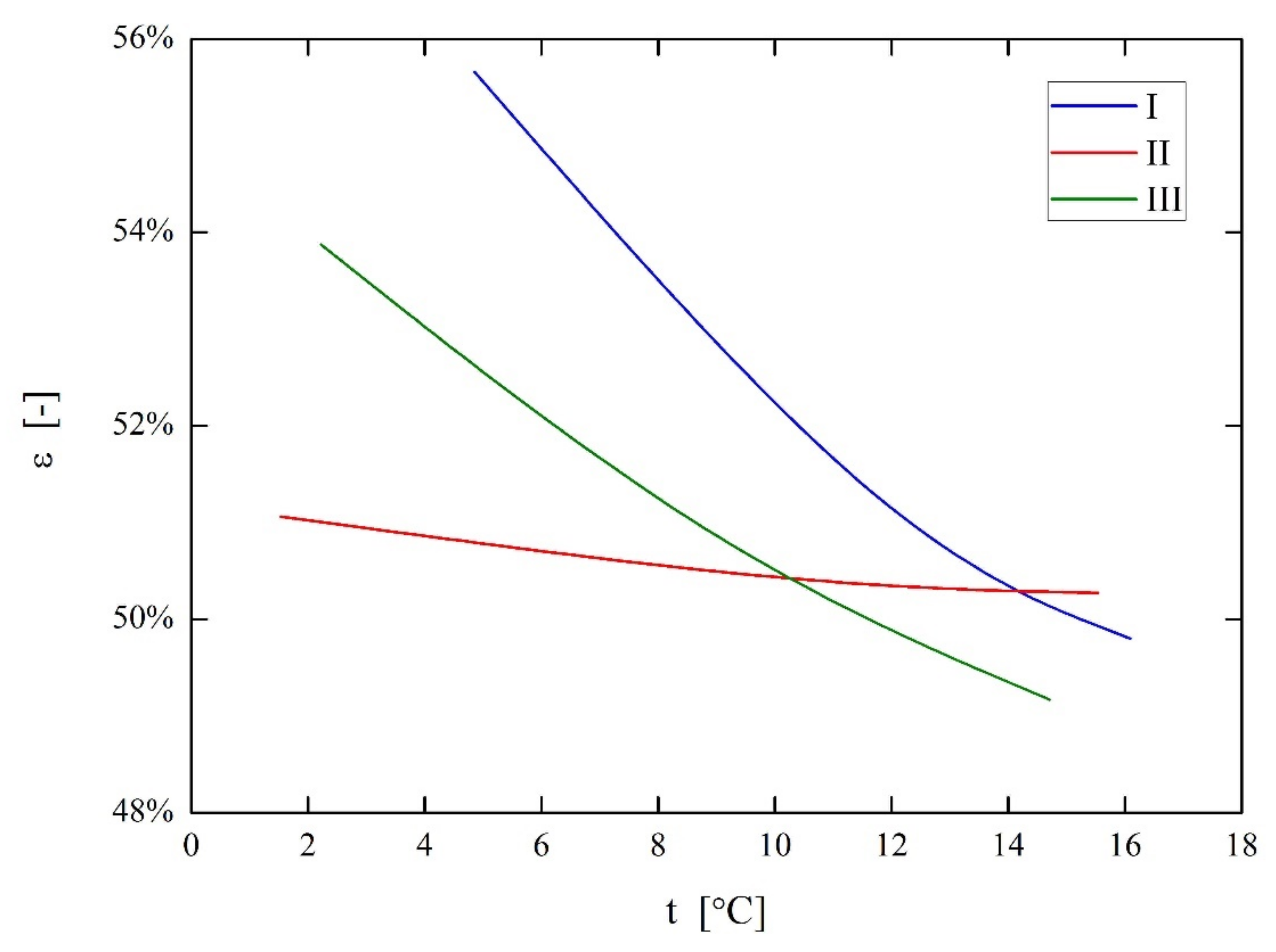
Figure 24 shows the values of the temperature effectiveness of the heat exchanger ε. Effectiveness depends on the fresh air inlet temperature. The graph shows the characteristics for three cases, characterized by different average volumetric flow rates in the air-ducts.
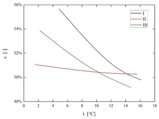
Figure 24.
HEX temperature effectiveness vs. the fresh air inlet temperature for different volumetric flow rates.
Based on the characteristics in Figure 24, it is possible to determine the ranges of the temperature effectiveness in the case of the tested HEX. The highest temperature effectiveness was recorded for the first measurement series (56%). The lowest temperature effectiveness of 49.2% was observed for measurement series characterized by the lowest volumetric airflow rates. The recorded temperature effectiveness was in the range of 49–56%. The temperature effectiveness decreased with increasing the fresh air temperature for all measurement series.
4. Discussion
The present work was aimed at the parametric design of HPHE aided by the computational model. The model was validated against the experiment on a nine-row prototype HPHE. There was a good agreement between the model and measured heat transfer rates of the prototype HPHE. Process and design specifications were made for HPHE utilized as an air-to-air recuperator for air conditioning systems. This HEX type implies the following design parameters:
The HP container is a 1 mm thick 20 mm outer diameter copper tube, and the finned surface is made of aluminum. Finned tubes are manufactured by cold rolling technology. Aluminum was chosen because of its lower weight than copper, and considerably lower price.
The computational model was used to obtain the heat transfer rates, effectiveness, and pressure drop for varying parameters. The first set of calculations with assumed constant inlet and outlet air temperatures was analyzed to choose a number of rows that fulfills the 60% thermal efficiency goal: 20 rows were chosen (including three extra HPS as a safety factor in calculations). In this arrangement (for 300 m3/h volumetric flow of hot and cold airstreams), the pressure drop does not exceed 100 Pa, increasing the maximal temperature difference of HPHE decreases in ΔP, with a relatively slight increase in effectiveness. The penalty for a reduction in temperature difference is not great as effectiveness drops by 4% over a 20 °C decrease. To sum up, a 20-rows HPHE exhibits stable effectiveness over a broad temperature range with an acceptable pressure drop for small air conditioning applications.
Further parametric computations were made to choose the optimal spacing between the HPs—3D plots show the dependence of efficiency and pressure drop on Xl and Xt. Traversal heat pipes spacing has the greatest influence on heat transfer rate; upon reduction in traversal spacing there is a steep increase in heat transfer rate and effectiveness for Xt ≈ 61 mm caused by the increase in the number of HPs in rows. Four and three pipe arrangement can be used (70 HPs total) instead of three and two (50 HPs total). Xt = 50 was chosen as the most effective transverse spacing between HPs, which corresponds to the physical contact of HPs. Smaller Xl means a shorter heat exchanger but also a higher pressure drop (Figure 23). To minimize the pumping power of the fan longitudinal spacing Xl = 61 mm was chosen. It corresponds to the total length of the heat exchanger, L2 = 1.22 m.
The final dimensions of the designed heat pipe heat exchanger are:
Length L2 = 1.22 m; Height L1 = 0.245 m, Width L3 = 0.245 m.
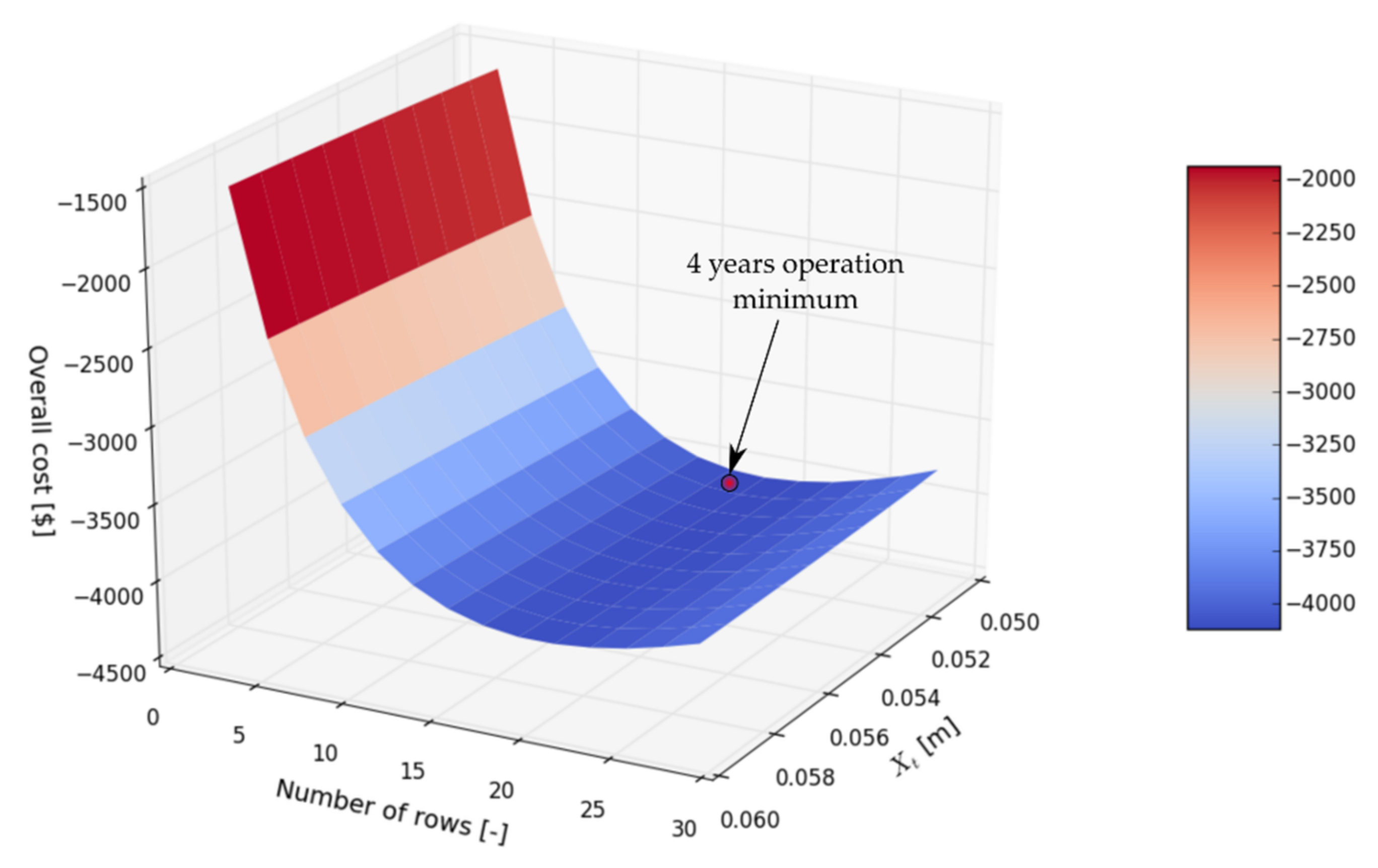
The final finned heat pipe arrangement is shown in Figure 25. Table 4 and Table 5 summarize HPHE working parameters for typical winter and summer conditions. The present best HPHE geometrical parameters choice is supported by the optimization of the overall cost function, which could be simplified to:
where N—a number of HPs in an HPHE. The cost of the manufacture of one heat pipe was estimated as USD 21, and the value of the working fluid inside one HP is approx. USD 1.5. The cost of the fan operation is estimated, assuming a fixed price of 1 kWh of electricity (0.2 USD/kWh). The first two terms in Equation (27) generate cost—initial cost of manufacture of HPHE plus the consumed electric energy for the fans’ operation. The savings come from the last term which takes into account the heat recuperation—in the cold months, the recuperated amount of thermal energy is priced as electrical energy (use of electrical heater), whereas in hot months, recuperated energy is divided by the Coefficient of Performance of the refrigeration device hypothetically used for airstream cooling. Based on the heat transfer rates, pressure drops, and air volumetric flow rate from the numerical model, the overall cost of HPHE in operation for 4 years is plotted in Figure 26. The chosen independent parameters were number of rows and traversal spacing Xt. The longitudinal spacing does not affect heat transfer or pressure drop significantly, so it was excluded from the analysis. The optimization method used to minimize the overall cost function is the so-called “brute force” method. The function’s value is computed at each point of a multidimensional grid of points, to find the global minimum. An obvious disadvantage of this approach is the high computing power requirements, but the advantage is a certainty of obtaining the minimum in the range of the specified parameters. The minimum is marked in Figure 26, being USD −4218 (a negative value means that the savings are greater than the cost of the investment) for 18 rows HPHE, and optimal spacing Xt = 0.051 m. It is very similar to the final dimensions of the HPHE chosen according to previous engineering analysis.
overall cost=HP cost·N + cost of fan operation − savings due to heat recuperation
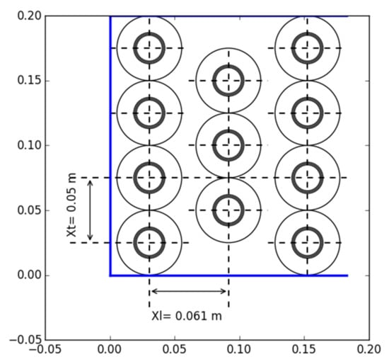
Figure 25.
Final heat pipe heat exchanger arrangement.
Table 4.
Final HPHE working parameters for typical summer conditions.
Table 5.
Final HPHE working parameters for typical winter conditions.

Figure 26.
The overall cost of 4 years of operation of HPHE as a function of number of rows and traversal HPs spacing.
5. Conclusions
The final parameters given in Table 4 and Table 5 prove that the designed 20-row individually finned HPHE is characterized by high recuperation effectiveness (55–65%). The effectiveness and heat transfer rate is higher for winter conditions, where higher temperature differences between airstreams exist.
The designed HPHE made of an individually finned HPs bundle is a competitive solution to the continuous plate-fine HPHE. The continuous fin HEX is a more thermally efficient construction (smaller number of rows for the same heat transfer rate), although the individual finning has its advantages in HPHE:
- -
- It is more durable—can withstand higher pressure differences on the airside;
- -
- Circular fins are less susceptible to mechanical damage than continuous fins, which can be easily deformed;
- -
- Individual finning allows for simple identification of damaged HPs in the bundle and their replacement;
- -
- HPHE with individually finned HPs can be more easily cleaned than continuously finned, therefore it is more robust in flue gas recuperation.
Even though more common continuous finned HPHEs outperform individually finned constructions, taking into account the above advantages, the construction proposed by authors can be more desired, especially from the exploitation and maintenance perspective.
The heat transfer intensification by the utilization of turbulators in an individually finned tube bundle (between HPs) is an attractive research direction, as it is not a widely recognized topic in the literature. It could improve the HPHE effectiveness significantly.
6. Patents
Polish patent number: P.415828, “Two-phase thermosiphon heat exchanger”, date 16-08-2018.
Author Contributions
Conceptualization, M.Ł. and G.G.; Methodology, M.Ł.; Software, M.Ł., A.N.G., and A.R.; Supervision, G.G.; Visualization, G.G., D.A., and B.W.; Writing—original draft, M.Ł., G.G., and M.K.; Writing—review and editing, A.N.G. All authors have read and agreed to the published version of the manuscript.
Funding
Research funded by the National Centre for Research and Development, research project LIDER (grant no. LIDER/08/42/L-3/11/NCBR/2012) “Intensification of the heat transfer process in innovative heat exchanger—investigation with the utilization of PIV method”.
Conflicts of Interest
The authors declare no conflict of interest.
Nomenclature
| A | heat transfer surface area, m2 |
| Af | finned area of the tube, m2 |
| Ao | minimum flow area, m2 |
| Ar | root (unfinned) area of the tube, m2 |
| As | area of finned surface, m2 |
| df | circular fin diameter, m |
| do, di | outside and inside HP diameter, m |
| dr | fin root diameter, m |
| f | friction coefficient, - |
| h | heat transfer coefficient, W/(m2∙K) |
| hca, hha | cold and hot air heat transfer coefficients, W/(m2∙K) |
| I0, I1 | modified Bessel function of order 0 and 1 |
| k | thermal conductivity, W/(m∙K) |
| K0, K1 | modified Bessel function K of order 0 and 1 |
| lf | fin length, m |
| L | length of HP, m |
| L1, L2, L3 | height, length, and width of HEX, m |
| m | the coefficient for fin efficiency—Equation (20), - |
| N | number of HPs in HPHE bundle, - |
| Nf | number of fins per unit length, 1/m |
| Nt | number of heat exchanger tube rows, - |
| Nu | Nusselt number, - |
| p | pressure, Pa |
| heat transfer rate through heat pipe, W | |
| ro, ri | outer and inner diameter of a circular fin, m |
| R | thermal resistance, K/W |
| Rca | convective thermal resistance of cold air flow, K/W |
| Rha | convective thermal resistance of hot air flow, K/W |
| Rhp | inside resistance of HP, K/W |
| Rfinned | overall thermal resistance of the finned surface, K/W |
| Rtube | thermal resistance of tube, K/W |
| Red | Reynolds number based on diameter, - |
| s | fin spacing, m |
| tf | fin thickness, m |
| tco, tci | outlet and inlet cold air stream temperature, °C |
| tho, thi | outlet and inlet hot air stream temperature, °C |
| T | temperature, K |
| Tm | enthalpy mixed-mean-temperature, K |
| U | overall heat transfer coefficient, W/(m2 |
| volumetric flow rate, m3/s | |
| wmax | maximal average velocity through a finned tube bundle, m/s |
| x, y, z | cartesian coordinates, m |
| x’, y’, z’ | the distance between HPs according to Figure 6 and Equations (11) and (12) |
| Xt | traversal spacing between tube centers, m |
| Xl | longitudinal spacing between tube centers, m |
Greek Symbols
| Δp | a pressure drop, Pa |
| εo | overall finned surface efficiency, - |
| ηf | fin efficiency, - |
| ν | kinematic viscosity, m2/s |
| ρ | density, kg/m3 |
Abbreviations
| HEX | heat exchanger |
| HP | heat pipe |
| HPHE | heat pipe heat exchanger |
| SHP | separate heat pipe |
References
- Reay, D.A.; David, A.; Kew, P.A.; Peter, A.; Dunn, P.D.; Peter, D. Heat Pipes; Butterworth-Heinemann: Oxford, UK, 2006; ISBN 9780080464770. [Google Scholar]
- Liu, D.; Tang, G.F.; Zhao, F.Y.; Wang, H.Q. Modeling and experimental investigation of looped separate heat pipe as waste heat recovery facility. Appl. Therm. Eng. 2006, 26, 2433–2441. [Google Scholar] [CrossRef]
- Srimuang, W.; Amatachaya, P. A review of the applications of heat pipe heat exchangers for heat recovery. Renew. Sustain. Energy Rev. 2012, 16, 4303–4315. [Google Scholar] [CrossRef]
- Tian, E.; He, Y.L.; Tao, W.Q. Research on a new type waste heat recovery gravity heat pipe exchanger. Appl. Energy 2017, 188, 586–594. [Google Scholar] [CrossRef]
- Hughes, B.R.; Chaudhry, H.N.; Calautit, J.K. Passive energy recovery from natural ventilation air streams. Appl. Energy 2014, 113, 127–140. [Google Scholar] [CrossRef]
- Abd El-Baky, M.A.; Mohamed, M.M. Heat pipe heat exchanger for heat recovery in air conditioning. Appl. Therm. Eng. 2007, 27, 795–801. [Google Scholar] [CrossRef]
- Noie, S.H. Investigation of thermal performance of an air-to-air thermosyphon heat exchanger using ε-NTU method. Appl. Therm. Eng. 2006, 26, 559–567. [Google Scholar] [CrossRef]
- Wu, X.P.; Johnson, P.; Akbarzadeh, A. Application of heat pipe heat exchangers to humidity control in air-conditioning systems. Appl. Therm. Eng. 1997, 17, 561–568. [Google Scholar] [CrossRef]
- Righetti, G.; Zilio, C.; Longo, G.A. Comparative performance analysis of the low GWP refrigerants HFO1234yf, HFO1234ze(E) and HC600a inside a roll-bond evaporator. Int. J. Refrig. 2015, 54, 1–9. [Google Scholar] [CrossRef]
- Jadhav, T.S.; Lele, M.M. Experimental performance and parametric analysis of heat pipe heat exchanger for air conditioning application integrated with evaporative cooling. Heat Mass Transf. und Stoffuebertragung 2017, 53, 3287–3293. [Google Scholar] [CrossRef]
- Rajski, K.; Danielewicz, J.; Brychcy, E. Performance Evaluation of a Gravity-Assisted Heat Pipe-Based Indirect Evaporative Cooler. Energies 2020, 13, 200. [Google Scholar] [CrossRef] [Green Version]
- Yau, Y.H.; Ahmadzadehtalatapeh, M. Performance Analysis of a Heat Pipe Heat Exchanger Under Different Fluid Charges. Heat Transf. Eng. 2014, 35, 1539–1548. [Google Scholar] [CrossRef]
- Vasiliev, L.L. Heat pipes in modern heat exchangers. Appl. Therm. Eng. 2005, 25, 1–19. [Google Scholar] [CrossRef]
- Yang, J.; Zhao, Y.; Chen, A.; Quan, Z. Thermal Performance of a Low-Temperature Heat Exchanger Using a Micro Heat Pipe Array. Energies 2019, 12, 675. [Google Scholar] [CrossRef] [Green Version]
- Yang, K.-S.; Jiang, M.-Y.; Tseng, C.-Y.; Wu, S.-K.; Shyu, J.-C. Experimental Investigation on the Thermal Performance of Pulsating Heat Pipe Heat Exchangers. Energies 2020, 13, 269. [Google Scholar] [CrossRef] [Green Version]
- Brough, D.; Ramos, J.; Delpech, B.; Jouhara, H. Development and validation of a TRNSYS type to simulate heat pipe heat exchangers in transient applications of waste heat recovery. Int. J. Thermofluids 2021, 9, 100056. [Google Scholar] [CrossRef]
- Yau, Y.H.; Ahmadzadehtalatapeh, M. Predicting yearly energy recovery and dehumidification enhancement with a heat pipe heat exchanger using typical meteorological year data in the tropics. J. Mech. Sci. Technol. 2011, 25, 847–853. [Google Scholar] [CrossRef]
- Yu, Z.T.; Hu, Y.C.; Cen, K.F. Optimal design of the separate type heat pipe heat exchanger. J. Zhejiang Univ. Sci. 2005, 6, 23–28. [Google Scholar] [CrossRef]
- Righetti, G.; Zilio, C.; Mancin, S.; Longo, G.A. Heat Pipe Finned Heat Exchanger for Heat Recovery: Experimental Results and Modeling. Heat Transf. Eng. 2018, 39, 1011–1023. [Google Scholar] [CrossRef]
- Thulukkanam, K. Heat Exchanger Design Handbook, 2nd ed.; Mechanical Engineering, CRC Press: Boca Raton, Florida, USA, 2013; ISBN 1439842124. [Google Scholar]
- Briggs, D.E.; Young, E.H. Convection heat transfer and pressure drop of air flowing across triangular pitch banks of finned tubes. Proc. Chem. Eng. Prog. Symp. Ser. 1963, 59, 1–10. [Google Scholar]
- Gorecki, G. Investigation of two-phase thermosyphon performance filled with modern HFC refrigerants. Heat Mass Transf. 2018, 54, 2131–2143. [Google Scholar] [CrossRef] [Green Version]
- Łęcki, M.; Górecki, G. Different approaches to FVM method fluid flow and heat transfer simulation inside thermosyphon. In Proceedings of the 15th International Heat Transfer Conference, Kyoto, Japan, 10–15 August 2014. [Google Scholar]
- Rura Bimetalowa Wysokożebrowana RBW—Cemal.com.pl—Najwyższej Jakości rury Żebrowane. Available online: http://cemal.com.pl/oferta/rura-bimetalowa-wysokozebrowana-rbw/ (accessed on 15 December 2020).
- Climate Meter LB-580—Multiparameter|ClimateLoggers.com. Available online: https://climateloggers.com/en/lb580-climate-meter.measuring-systems.html (accessed on 16 August 2021).


Publisher’s Note: MDPI stays neutral with regard to jurisdictional claims in published maps and institutional affiliations. |
© 2021 by the authors. Licensee MDPI, Basel, Switzerland. This article is an open access article distributed under the terms and conditions of the Creative Commons Attribution (CC BY) license (https://creativecommons.org/licenses/by/4.0/).