
Numerical Modelling of Heat Transfer in Fine Dispersive Slurry Flow


Division of Production Engineering, Faculty of Management and Computer Modelling, Kielce University of Technology, Al. Tysiaclecia P.P. 7, 25-314 Kielce, Poland
Energies 2021, 14(16), 4909; https://doi.org/10.3390/en14164909
Submission received: 21 July 2021
/
Revised: 6 August 2021
/
Accepted: 8 August 2021
/
Published: 11 August 2021
(This article belongs to the Special Issue Numerical Heat Transfer and Fluid Flow 2021)
Abstract
:Slurry flows commonly appear in the transport of minerals from a mine to the processing site or from the deep ocean to the surface level. The process of heat transfer in solid–liquid flow is especially important for the long pipeline distance. The paper is focused on the numerical modelling and simulation of heat transfer in a fine dispersive slurry, which exhibits yield stress and damping of turbulence. The Bingham rheological model and the apparent viscosity concept were applied. The physical model was formulated and then the mathematical model, which constitutes conservative equations based on the time average approach for mass, momentum, and internal energy. The slurry flow in a pipeline is turbulent and fully developed hydrodynamically and thermally. The closure problem was solved by taking into account the Boussinesque hypothesis and a suitable turbulence model, which includes the influence of the yield shear stress on the wall damping function. The objective of the paper is to develop a new correlation of the Nusselt number for turbulent flow of fine dispersive slurry that exhibits yield stress and damping of turbulence. Simulations were performed for turbulent slurry flow, for solid volume concentrations 10%, 20%, 30%, and for water. The mathematical model for heat transfer of the carrier liquid flow has been validated. The study confirmed that the slurry velocity profiles are substantially different from those of the carrier liquid and have a significant effect on the heat transfer process. The highest rate of decrease in the Nusselt number is for low solid concentrations, while for C > 10% the decrease in the Nusselt number is gradual. A new correlation for the Nusselt number is proposed, which includes the Reynolds and Prandtl numbers, the dimensionless yield shear stress, and solid concentration. The new Nusselt number is in good agreement with the numerical predictions and the highest relative error was obtained for C = 10% and Nu = 44.3 and is equal to −12%. Results of the simulations are discussed. Conclusions and recommendations for further research are formulated.
1. Introduction
Slurry pipeline transport is widely used in the food and chemical industry and in the transfer of minerals from a mine to the processing site or from the deep ocean to the surface level [1]. Pipeline transportation is more economical and environmentally friendly than other modes of transport, such as rail or trucking, when moving minerals over long distances. They also have a high safe delivery rate [2,3]. In the literature, we can find various approaches for the analysis of solid–liquid flow and its predictions [4,5,6,7,8,9,10,11,12,13,14]. Analyses are mainly dedicated to a proper class of flow, such as homogeneous, heterogeneous, and with steady or mowing beds. The proposed models are mainly algebraic. If predictions are considered, we use analytical or numerical methods [15,16,17,18,19,20,21,22,23,24]. Analytical methods are impractical and can be applied to very simple flow conditions. If numerical methods are considered, we recognize Direct Numerical Simulation (DNS), which is computationally costly, Large Eddy Simulation (LES), which is less expensive, Reynolds-averaged Navier–Stokes equations (RANS), which is the computationally cheapest, or a combination of the mentioned methods, called hybrid methods. The slurry flow phenomenon is very complex; therefore, mathematical models are strictly dedicated to a certain flow situation.
The heat transfer process in slurry transportation is essential, especially for long distances. Temperature affects the viscosity and rheological properties of the slurry and thus changes the energy loss during pipeline transport, which affects the operation of the pipeline system. Changes in the temperature of the transported slurry can be caused by heat transfer between the slurry pipeline and the environment and by the conversion of part of the mechanical energy into heat. In the case of pipeline operation in the Arctic Sea, for example, it could cause permafrost melting and instability of pipeline routes. In other cases, maintaining a constant temperature of the flowing medium is imperative, while in some other cases, the risk of freezing or loss of heat appears, which requires proper pipe insulation to avoid plug formation. Therefore, the ability to predict the flow of the slurry with heat exchange is a great challenge in CFD.
To predict the heat transfer between the flowing slurry and the environment, the first point is to set up a reliable physical model and then a mathematical model. The mathematical model should be able to predict the velocity and temperature fields of the slurry. When formulating a physical model for slurry flow with heat transfer, it is necessary to define the slurry properties and flow conditions like, for instance:
- -
- particle size distribution and its shape, elasticity, porosity, degradation, hydrophobicity, averaged solid particle diameter and density;
- -
- carrier liquid viscosity and density;
- -
- type of slurry: Newtonian or non-Newtonian, with or without yield stress;
- -
- type of solid concentration: dilute suspension or highly concentrated;
- -
- type of slurry flow: laminar, transient, turbulent, homogeneous, pseudo-homogeneous, heterogeneous, with steady or moving beds;
- -
- geometry and flow direction: circular or noncircular conduit, one-, two-, or three-dimensional, vertical, horizontal, or inclined conduit;
- -
- boundary conditions for velocity and temperature;
The study focuses on the modelling and simulation of convective heat transfer between a fine dispersive slurry and a pipe wall under a turbulent flow regime in a range of solid concentrations for commercial applications. The solid phase constitutes fine solid particles with an average diameter of about 20 μm, since small particles are responsible for increasing viscosity, non-Newtonian behavior, and damping of turbulence. Therefore, the relation between shear stress and shear rate is crucial to include in a mathematical model.
Solid particles are known to affect the flow structure and can enhance or suppress turbulence [25,26,27,28,29,30,31,32,33]. Generally, one can conclude that small particles can suppress, while large particles can increase turbulence. Of course, the phenomenon is more complex as the particle density, carrier liquid properties, and flow conditions, such as the velocity and geometry effect on the level of turbulence as well. Experimental data on frictional head loss for turbulent flow of fine dispersive slurry clearly demonstrate a lower frictional head loss than expected [6,25,34,35]. Wilson and Thomas hypothesized that in a turbulent flow of fine dispersive slurry, the viscous sublayer becomes thicker compared to a single-phase flow under the same flow conditions [25]. Therefore, the Wilson and Thomas hypothesis was taken into account to develop a mathematical model.
Considering the heat exchange between the transported slurry and the surrounding, we recognize methods and techniques focused on the enhancement of heat exchange, named passive or active. Passive methods, such as shape insert with dedicated perforation or mechanically deformed pipes, have been studied for several years and have become commercial solutions [36,37,38,39,40,41]. Active methods, such as air injection, bubble generation, or proper pulsation, can produce increases in the heat transfer process [42,43,44,45].
Heat transfer in the solid–liquid flow has been experimentally investigated by several studies [46,47,48,49]. However, experiments and studies on heat transfer in a turbulent flow with fine solid particles, especially for solid concentrations of commercial interest, above 20% by volume, are scattered in the literature. Existing experiments refer mainly to water-air or water-oil or nanofluids or slurries with low solid concentrations [50,51,52,53]. Research mainly includes solid particles made of metals, oxides, or carbides suspended in a liquid. Such experiments and predictions focus on examining whether solid particles can increase or decrease the heat transfer process between the suspension and a pipe wall. The results show that such an increase depends mainly on the properties of the particles and the solid concentration [54,55].
Wang et al. [48] experimentally examined the thermal conductivity of Al2O3 and CuO nanoparticles mixed with water, vacuum pump liquid, engine oil and ethylene glycol. The average particle diameter of Al2O3 was 28 nm and the average particle diameter of CuO was 23 nm. All particles were loosely agglomerated in the chosen liquid. Experiments have shown that the heat transfer of the mixture increases with the volume fraction of Al2O3 particles [48].
Rozenblit et al. [56] conducted an experimental study on the heat transfer coefficient associated with solid–liquid transport in a horizontal pipe using an electro-resistance sensor and infrared imaging. They considered a flow of acetyl-water mixture on a moving bed with solid volume concentrations of 6%, 9%, 12%, and 15% by volume. They noted that the local heat transfer coefficient changes from its lowest value at the bottom of the pipe to its highest value above the carrier liquid at the upper heterogeneous layer. These experiments indicated that the heat transfer coefficient is strongly influenced by the cross-sectional distribution of the solid phase [56].
Ku et al. [49] experimentally examined the effect of solid particles on heat transfer. They used spherical fly ash particles with a mass median particle diameter of 4 to 78 μm and a particle density of 2270 kg/m3, and Reynolds numbers of 4000 to 11,000 in an 8 mm inner diameter pipe. The authors noted that the highest heat transfer coefficient was obtained for the dilute solution with C = 3%, and then gradually decreased with increasing solid volume concentration. They proposed a correlation for the Nusselt number. The correlation depends on Reynolds and Prandtl numbers, solid concentration, and the ratio of pipe diameter to average particle diameter. The correlation is limited to: Re = 3000–11,000; Pr = 3.8–5.0; D/dP = 102–615; C = (1–10)%. However, it is not clear whether such suspensions possess or do not possess the yield stress. Furthermore, the apparent viscosity of the slurry in their research was 1.75 higher compared to water if C = 30%. This contrasts with current studies, as the apparent viscosity of C = 30% is at least 13 times higher compared to water and increases as the wall shear stress decreases. Additionally, the Prandtl number in the current study is much higher compared to the limitation of Ku et al. 49]. In conclusion, we can say that it is impossible to compare the numerical predictions with the experimental data if the slurry properties differ much.
Bartosik performed simulations of the influence of the solid volume concentration [57] and the yield shear stress [58] on heat transfer in kaolin slurry. The author considered two solid concentrations of kaolin equal to 7.4% and 38.3%, which correspond to yield shear stresses of 4.92 Pa and 9 Pa, respectively. The author found that both solid concentration and yield stress strongly affect the Nusselt number and the Nusselt number decreases with increasing solid concentration or yield stress.
Analysis of the literature indicates that most of the research deals with heat transfer in a single phase, liquid-air flow, nanofluids, ice slurry, laminar flow, or with low solid concentrations. Experiments and modelling of heat transfer in non-Newtonian slurries containing minerals with fine particles, yield stress, and solid volume concentration at least 20% by volume are scattered. Reliable predictions require reliable measurements. Prediction difficulties arise when the solid concentration increases and the particle-liquid and/or particle–wall interaction occurs. A better approach to understanding the slurry flow mechanism and its correlation with the heat transfer process, especially at high solid concentrations, is needed, as it is important for better optimization design and operation control. The ability to simulate turbulent solid–liquid flow to predict frictional head loss, velocity, and temperature distributions remains one of the main challenges in CFD. However, from an engineering point of view, we need simple empirical or semiempirical correlations that allow the calculation of the heat transfer coefficient for known slurry. Therefore, proper correlations for the Nusselt number are still required.
The objective of the paper is to develop a new correlation of the Nusselt number for turbulent flow of fine dispersive slurry that exhibits yield stress and damping of turbulence. For such a slurry, a new correlation of the Nusselt number is proposed. The new correlation of the Nusselt number includes Reynolds and Prandtl numbers, solid volume concentration, and dimensionless yield shear stress.
2. Physical Model
The slurry is assumed to be a mixture of fine solid particles and water, which plays the role of a carrier liquid. The assumptions made in the physical model are as follows:
- -
- solid particles are round, smooth, rigid, non-hydrophobic, and the influence of such properties on slurry flow is not considered;
- -
- solid particles are sufficiently fine, with a median particle diameter dP ≅ 20 μm, so the damping of turbulence, described by Wilson and Thomas [25], occurs;
- -
- the slurry flows in a straight and smooth horizontal pipeline, which is rigid and its inner diameter is constant;
- -
- -
- the rheological properties of the slurry can be approximated by the Bingham model;
- -
- the flow of the slurry is turbulent, steady, axially symmetric (V = 0) and without circumferential eddies (W = 0);
- -
- the slurry flow is fully developed hydrodynamically, which means that the time-averaged velocity component U does not change in the flow direction (∂U/∂x = 0).
- -
- the wall temperature is steady;
- -
- the heat flux is homogeneous; the heat flux acts from the slurry to the pipe wall; its value is steady, known, and sufficiently small, so the following arbitrarily chosen condition is met: |Tb − Tw|< 7 K;
- -
- the apparent viscosity and specific heat are constant and are determined by the thermal condition at the pipe wall, while the slurry density and conduction coefficient are calculated from the bulk temperature;
- -
- there is no inner heat production in a slurry, and conversion of mechanical energy into internal heat is not considered;
- -
- heat due to radiation and conduction through a pipe wall are negligible;
- -
- the slurry flow is fully developed thermally, which means that the temperature changes linearly in the flow direction ‘ox’ (∂T/∂x = const ≠ 0).
For simulation purposes, the cylindrical coordinate system is used, where ‘ox’ is the main flow direction, while ‘or’ is the radial coordinate, as presented in Figure 1. It is assumed that the wall temperature is equal to Tw = 293.15 K, and the heat flux density q = −500 W/m and both quantities are steady. Simulations are performed for carrier liquid flow (C = 0%) and for slurry with a solid particle density equal to 2550 kg/m3, solid concentrations 10%, 20%, 30% and for an inner pipe diameter D = 0.02 m.
3. Mathematical Model
The starting points for building a mathematical model for non-isothermal slurry flow in a pipeline are continuity, Navier–Stokes, and internal energy equations. A mathematical model is formulated for Newtonian liquid and non-Newtonian slurry.
3.1. Newtonian Liquid
The mathematical model for the Newtonian liquid regards the carrier liquid, which is pure water. Taking into account the time-averaged procedure proposed by Reynolds [60], and neglecting terms with fluctuations of density and viscosity, it is possible to obtain the conservative equations of mass, momentum, and internal energy as follows:
where the Prandtl number in Equation (3) is defined as follows:
The momentum Equation (2), also named the Reynolds Averaged Navier–Stokes equation, possesses an additional term , which appears on the right-hand side, named turbulent stress tensor or Reynold’s stress tensor. It is a symmetric tensor and requires additional equations to calculate its components. To solve the set of equations, the number of dependent variables must be the same as the number of equations, which is called the closure problem. Therefore, additional equations are proposed that allow one to calculate the components of the turbulent stress tensor. Equation (3) possesses an additional term This term is responsible for the intensification of heat exchange caused by the presence of velocity and temperature fluctuations and requires closure, too. The additional terms in Equations (2) and (3) can be modelled by a direct approach (DNS) or an indirect approach. To calculate each component of and the direct or indirect methods require additional equations, either algebraic or partial differential. Although DNS and LES methods can give a high level of accuracy, they are time-consuming and computationally costly. Indirect methods can give accurate predictions with less computational power. Moreover, we deal with time-averaged quantities of velocity and temperature, instead of random quantities, which are more useful to engineers. For this study, an indirect method is employed. The indirect method employs the Boussinesque hypothesis, which introduced a new dependent variable, called turbulent viscosity, as a measure of turbulence rather than viscosity [61]. The Boussineque hypothesis assumes that the turbulent stress tensor in Equation (2) can be expressed as follows:
and the fluctuating components of velocity and temperature in the energy Equation (3), as:
The turbulent Prandtl number (Prt) in Equation (6) was intensively examined by several researchers. Studies indicated that in the flow on a plate, Prt ≅ 0.5, while for the boundary layer, which exists in a pipe flow, the turbulent Prandtl number is estimated to be Prt = 0.9 [62].
If an axially symmetric flow is considered, the most suitable coordinate system is cylindrical, where the dependent variables are functions of x, r, θ. The assumption that the flow is axially symmetric causes the velocity component V = 0. The lack of circumferential eddies causes that component of the velocity W = 0. The last term on the right-hand side of Equation (2) is also zero because the flow is horizontal.
Taking into account the assumptions stated in the physical model, the time-averaged Equations (1)–(3) together with (5), (6) can be formulated in the final form as follows:
Taking into account the assumption that the flow is fully developed thermally, which means that the temperature changes linearly in the main flow direction ‘ox’, the convective term in Equation (9) will be delivered by an energy balance. An energy balance is developed for the slurry flowing in a tube with inner diameter D and unit length L = 1 m. Such an approach simplifies the mathematical model to one-dimensional and substantially reduces the time of computation.
Let us consider a heat flux acting between the flowing liquid and a pipe—Figure 1.
where
and is temperature difference on radius r.
The change in the inner energy of the flowing liquid at distance L is the following:
where the pipe cross section A = πD2/4, and is the slurry temperature difference at distance x = L.
Comparing (10) and (12), we can write:
Dividing each side of Equation (13) by the unit length of the pipe L, we can write:
where the heat flux density can be written as:
The final form of the convective term can be established using Equation (14), as follows:
The convective term (16) delivered from the energy balance replaces the convective term on the left-hand side of Equation (9). Taking into account Equation (16), one can say that the convective term ∂T/∂x = 0 if q = 0. The heat flux acting on the pipeline is positive if Tw > Tb or negative if Tw < Tb. The thermal properties of the slurry are treated as known quantities and will be presented. The influence of temperature on a carrier liquid density and a thermal conductivity was approximated using the Taylor expansion as follows:
while slurry properties, such as density, coefficient of heat conduction, and specific heat, were calculated as follows:
Finally, the mathematical model of heat transfer in liquid flow constitutes two partial differential equations, namely, (8) and (9), since the continuity Equation (7) is included in the momentum Equation (8), and the complementary Equation (16). Equation sets possess the following dependent variables: U(r), μt(r), p(x), T(r). To calculate the velocity and temperature profiles across a pipe, a set of equations requires closure. Turbulent viscosity μt(r) will be calculated using an indirect method together with a suitable turbulence model, while the pressure gradient ∂p/∂x will be treated as a known value. For the preset value of ∂p/∂x, the velocity and temperature profiles will be calculated. In other words, for known values of ∂p/∂x the time-averaged profiles of U and T will be calculated.
To calculate the turbulent viscosity μt(r), the Launder and Sharma turbulence model was chosen [63]. The chosen model fulfills the requirements formulated by Spalding [64,65], an honorable founder of Computational Fluid Dynamics (CFD). The Launder and Sharma model was successfully examined for comprehensive types of flow, including homogeneous slurries. The researchers emphasized that it is one of the first and most widely used models and has been shown to agree well with the experimental and DNS data for a wide range of turbulent flow problems, performing better than many other k–ε models [66,67,68,69].
The Launder and Sharma turbulence model assumes that the turbulent viscosity depends on the kinetic energy of the turbulence, defined by Equation (19), and the dissipation rate of the kinetic energy of the turbulence, defined for homogeneous turbulence by Equation (20) [70]. On the basis of dimensional analyzes, Launder and Sharma assumed that the turbulent viscosity depends on k, ε and ρ as follows:
where fμ is called the damping of the turbulence function or the wall function. The function causes a reduction in turbulent viscosity if y → 0. The wall function was developed empirically by matching the predictions with measurements and is the following:
where the turbulent Reynolds number (Ret) was developed from dimensionless analysis, as follows:
Equations for the kinetic energy of turbulence and its dissipation rate are obtained from the Navier–Stokes equations, using a time-averaged procedure [63].
Taking into account the assumptions made in the physical model, the final form of the equations for the kinetic energy of turbulence and its dissipation rate, in cylindrical coordinates, are as follows:
The set of partial differential Equations (8), (9), (24) and (25) together with the complementary Equations (16), (21)–(23) is dedicated to a Newtonian liquid.
3.2. Non-Newtonian Fine Dispersive Slurry
If non-Newtonian slurry is considered, the first step is to set up a suitable rheological model. According to the physical model, we consider a slurry with fine solid particles. It is well known that fine solid particles are responsible for increased viscosity and non-Newtonian behavior [6]. The slurry with fine solid particles can be described by several rheological models, like for instance, Bingham, Ostwalda–de Waele, Carreau, Casson, or Herschel–Bulkley. The Bingham model is very simple as it demonstrates the yield stress and constant viscosity. Two- and three-parameter models, such as Casson or Herschel-Bulkley, describe the influence of the shear rate on the shear stress more accurately. In the case of laminar flow, a rheological model plays a crucial role in determining shear stress, while in a turbulent flow the dominant role plays turbulence. Therefore, the Bingham model is used as a simpler one. It is also important that experimental data for such a model are available in the literature.
The Bingham rheological model is described by Equations (26) and (27), as follows:
and
Taking into account the right-hand side of Equations (26) and (28), the following equation for apparent viscosity can be obtained:
Of course, Equation (29) has the limitation that the yield shear stress cannot be equal to or higher than the wall shear stress. If the wall shear stress increases, the apparent viscosity decreases.
Considering the forces that act on the slurry flowing in a horizontal pipeline of length L and inner diameter D, we can write that the force responsible for the movement is:
while the resistance force is the following:
For a steady flow of slurry, both forces must be equal. Therefore, we can write:
Finally, for known plastic viscosity, yield stress and ∂p/∂x, the apparent viscosity can be calculated as follows:
Analyzing Equation (33) it can be concluded that for the Bingham model the apparent viscosity is constant across a pipe stream if ∂p/∂x = const and τo = const. To consider a non-Newtonian slurry, the coefficient of dynamic viscosity, which exists in Equations (8), (9) and (23)–(25), has to be replaced by the apparent viscosity, defined by Equation (33).
The mathematical model for isothermal flow, which constitutes Equations (8), (24) and (25) together with the complementary Equations (21)–(23) and (33) fails if the predictions of fine dispersive slurry flow, defined in the physical model, are considered. Such a slurry exhibits lower head loss than expected. Therefore, taking into account the Wilson and Thomas hypothesis [25], Bartosik [73] proposed a modified the wall function, defined by Equation (34). The wall Function (34) is important for a close distance to a pipe wall. For a turbulent Reynolds number greater than 100, the wall Function (34) gives similar results to the function defined by Equation (22). Now, the Equation (34) replaces Equation (22) proposed by Launder and Sharma.
Finally, the mathematical model for heat transfer in fine dispersive slurry flow constitutes the partial differential Equations (8), (9), (24) and (25), together with the complementary Equations (16), (21), (23), (33) and (34). The constants in the k-ε turbulence model are the same as in the Launder and Sharma model and are the following: C1 = 1.44; C2 = 1.92; σk = 1.0; σε = 1.3 [63].
4. Numerical Procedure
The mathematical model assumes the following boundary conditions:
at the pipe wall for r = R: T = Tw; q = const; U = 0; k = 0; ε = 0;
symmetry axis for r = 0: ∂T/∂r = 0; ∂U/∂r = 0, ∂k/∂r = 0 and ∂ε/∂r = 0.
The boundary condition (35) indicates that there is no sleep velocity, k and ε on the pipe wall (r = R). Very near the wall, the dissipation rate is equal to 2 μ(∂k0.5/∂r)2. This term was added to Equation (24) to allow to be set to zero on the pipe wall (y = 0). The boundary condition (36) indicates that axially symmetric conditions were applied to all dependent variables.
The set of partial differential Equations (8), (9), (24) and (25) was computed using a finite difference scheme and its own computer code. The set of equations was solved taking into account the TDMA approach, with an iteration procedure, and using the control volume method [74]. The control volume was obtained for a pipe of length equal to L = 1 m and rotating the radius of the pipe around the symmetry axis at an angle of 1 radian.
The calculations were carried out in a proper order. For the predetermined value of ∂p/∂x, the following inlet conditions were used:
- -
- T(r) = Tw;
- -
- U(r) = Umax[(R − r)/R]1/7, where Umax was arbitrarily chosen;
- -
- k was set up on the basis of the intensity of the assigned turbulence, that is, k(r) = ½ U2(r);
- -
- ε was established based of the relation: ε(r) = 0.093/4 k3/2(r)/L, where L was determined from the Nikuradse formula.
Attention was paid to the effect of the number of grid points localized across a radius of a pipe. It is well known that the number of nodal points strongly affects the accuracy of the predictions [74,75]. Therefore, the radius of the pipe was divided into 80 nodal points that were not uniformly distributed across the pipe. Most of the nodal points were located near the wall of the pipe. The number of nodal points was experimentally set to provide nodally independent predictions.
The iteration cycles were repeated until the convergence criterion, defined by Equation (37), was achieved.
where is a general dependent variable = U, T, k, ε; the jth is the nodal point after the nth iteration cycle and the is the (n − 1)th iteration cycle.
Finally, the hydrodynamically and thermally developed turbulent flow of the fine dispersive slurry was calculated and the following profiles were obtained: T(r), U(r), k(r), ε(r) and the following dependent variables were calculated: Ub, Tb, Re, Pr, Nu.
5. Validation of the Mathematical Model
The mathematical model for the isothermal flow of fine dispersive slurry has been validated in a comprehensive range of solid concentrations, yield stresses, Reynolds number and pipe diameters, providing fairly good predictions of frictional head loss and velocity profiles [20,21,73,76].
The validation of the heat transfer was performed only for the carrier liquid flow. Heat transfer validation for the fine dispersive slurry was not performed because, to the best knowledge of the author, no experimental data are available. Existing experiments and correlations of Nusselt number, made for instance, by Harada et al. [46], Ku et al. [49], Salamone and Newman [77], Ozbelge and Somer [78] do not take into account the slurry defined in the physical model.
Validation of heat transfer for carrier liquid flow includes the prediction of the Nusselt number. The results were compared with empirical data expressed by the Dittus–Boelter correlation [79]. The Dittus–Boelter correlation is valid for fully developed flow and for Re > 10,000 and 0.7 ≤ Pr ≤ 160 [79]. The Dittus–Boelter correlation is reasonably consistent with the experimental data [80,81] and is expressed as follows:
where Reynolds and Prandtl numbers were expressed for this study by Equations (39) and (40), respectively.
Of course, the apparent viscosity (μapp) in case of carrier liquid is equal to carrier liquid viscosity (μ).
The Dittus–Boelter correlation, expressed by Equation (38), approximates the physical situation quite well for the case of constant wall temperature and constant wall heat flux, which is just exactly as it is assumed in the physical model.
Figure 2 presents comparisons of the Nusselt number calculated using the mathematical model with the Dittus–Boelter correlation (38) for the carrier liquid in the range of Reynolds numbers of 6900 to 100,000. The results of the comparison presented in Figure 2 show good agreement; however, there are some discrepancies for low and high Reynolds numbers. The average relative error in the range of Re = 6900–100,000 is approximately −3.5%.
As mentioned above, the mathematical model for the isothermal flow of fine dispersive slurries, which exhibits turbulence damping, was successfully examined. The model is also positively verified for heat transfer in the carrier liquid flow—Figure 2. Therefore, it is assumed that the mathematical model is suitable for predicting the thermally fully developed flow of the fine dispersive slurry with constant wall heat flux and constant wall temperature.
6. Simulation Results
To perform simulations of heat transfer in a turbulent flow of a fine dispersive slurry, which is non-Newtonian and exhibits yield stress and turbulence damping, the rheological parameters must first be determined. Therefore, rheological measurements of Shook and Roco of a fine limestone slurry, with a solid density similar to that assumed in the physical model, were considered [6]. Because Shook and Roco experimental data are for a narrow range of solid concentrations, the Slatter measurements were used to extend the range of rheological parameters [82]. In the case of the Shook and Roco experiments, solid particles with diameter below 44 μm constitute 67%, while in the case of the Slatter experiment the median particle diameter was equal to 28 μm. Therefore, the assumption made in the physical model that the median particle diameter is about 20 μm is an estimation rather than a precise diameter determination.
The results of the approximation of the measurements of Shook and Roco [6] and Slatter [82] are collected in Figure 3a,b. Taking into account the approximation of the measurements, the yield stress and plastic viscosity have been estimated for solid volume concentrations equal to 10%, 20% and 30%. The rheological parameters of the slurry for the Bingham model are collected in Table 1.
Numerical simulations were performed for a constant heat flux that acts from the slurry to the pipe wall. The thermal properties of the solid and liquid phases are presented in Table 2. Simulations of heat transfer in turbulent flow of fine dispersive slurry were performed for solid volume concentrations equal to: 10%; 20%, 30% and for water. As a result, temperature and velocity profiles were obtained.
Figure 4a–c demonstrate the influence of solid concentration on the slurry temperature profiles at the same bulk velocity equal to 3.50 m/s. If the bulk velocity is constant, the temperature difference between the wall and the slurry increases significantly with increasing solid volume concentration. Therefore, considering Equation (15), it can be concluded that for the constant bulk velocity, the heat transfer coefficient decreases with increasing solid volume concentration because the density of heat flux and diameter of the pipe are constant. To confirm this, Figure 4d shows the influence of solid volume concentration on the Nusselt number for constant bulk velocity. It is assumed that if the calculations for C = 0% are presented, this means that there is a flow of pure water. At the same bulk velocity of the carrier liquid and slurry, it is seen that the highest rate of decrease in the Nusselt number is in the range of C = 0% to C = 10%, while for C > 10% the decrease in the Nusselt number is gradual.
If the slurry temperature distribution is known, the heat transfer coefficient can be found by calculating the density of heat flux at the slurry boundary as follows:
The velocity distribution plays an important role in the heat exchange process and affects the Nusselt number. The viscous sublayer plays a crucial role for shear stress and heat transfer, while the buffer layer exhibits the highest generation of turbulence, which improves diffusion processes and, as a consequence, the effects on the heat transfer rate [83,84]. For this reason, the slurry velocity profile analysis is useful.
The velocity profiles for constant bulk velocity are presented in Figure 5a–c for different solid concentrations. Slurry velocity profiles are compared with carrier liquid profiles at the same bulk velocity and under the same thermal conditions (q = const; Tw = const) and for the same pipe diameter. However, it should be emphasized that it is useless to compare the velocity profiles of the slurry and water for the same Reynolds number. In such a case, the velocity profiles are substantially different because the viscosities of the slurry and water differ considerably. Figure 5a–c indicate that the velocity gradient at the pipe wall is lower for the slurry than for the carrier liquid. Differences are strongly dependent on the solid concentration. To illustrate what happens at the wall of the pipe, Figure 5d presents the logarithmic profiles of dimensionless turbulent stresses, calculated as a turbulent to laminar stress ratio (μt/μapp), for slurry with C = 30% and for water. Again, predictions are made for a constant bulk velocity. It is seen that both profiles differ significantly. For R+ > 5, the dimensionless turbulent stresses are higher in the carrier liquid than in the slurry, which means that turbulent diffusion is greater in the water flow than in the slurry. This is a result of the high viscosity of the slurry. Taking into account the effect of velocity, we expect that for the same bulk velocity of the slurry and the carrier liquid, the heat transfer coefficient of the slurry should be lower than that of water.
The most practical way to calculate the heat transfer coefficient is to use the Nusselt number. Figure 6a presents the influence of Reynolds number on the Nusselt number for slurry and water. The Nusselt number is seen to be higher for the slurry than for the water and increases with increasing solid concentration. However, the rate of increase in the Nusselt number from 20% to 30% seems to be lower than from 10% to 20%. Figure 6b presents the influence of the bulk velocity on the Nusselt number. It is seen that, for the same bulk velocity, the Nusselt number is much lower than the Nusselt number for the carrier liquid, and differences arise as the solid concentration increases. This is in line with earlier conclusions withdrawn by analyzing Figure 4a–c and Figure 5a–c and with the conclusions of some researchers such as Rozenblit et al. [56], for instance.
From an engineering point of view, it is not practical to build a complex mathematical model to predict the heat transfer coefficient for the slurry flow. It is more practical for engineers to use a simple function, like the Nusselt number, which is defined as the ratio of convection to conduction of heat transfer. The Nusselt number allows for calculation of the heat transfer coefficient.
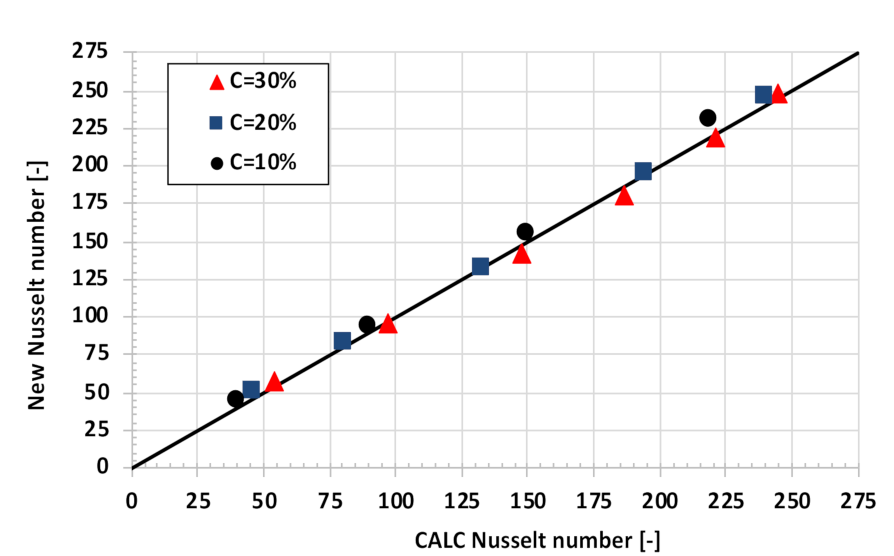
Based on simulations of thermally developed fine dispersive slurry flow, which exhibits yield stress and damping of turbulence in the range of solid volume concentration C = (10–30)% and for Tw = const and q = const, the following equation is developed for the Nusselt number:
Equation (42) was developed on the basis of the Nusselt number dedicated to water. The equation includes the properties of the slurry, such as solid volume concentration and dimensionless yield shear stress. Dimensionless yield shear stress was defined as the ratio of yield shear stress to wall shear stress. The wall shear stress can be easily calculated by Equation (32), for example. Equation (42) can be applied if τw > τo.
Figure 7 presents the calculation of a new Nusselt number, using the correlation expressed by Equation (42), versus the Nusselt number calculated from the mathematical model. The calculations using the new correlation (42) matched well with the numerical predictions. The discrepancy exists for low Nusselt numbers. As an example, for the lowest value of the Nusselt number and C = 30%, the relative error is equal to −6%, while for the highest Nusselt number it is equal to −1%. Taking into account the influence of solid concentration on the accuracy of the prediction by Equation (42), the highest relative error was observed for C = 10% and Nu = 44.3 and is equal to −12%.
7. Discussion and Conclusions
The heat transfer characteristics of the fine dispersive slurry, which exhibit yield stress and damping of turbulence, are not well understood. Experiments and modelling of such slurries are difficult. High-concentration slurry measurements are at risk of damage or contamination by intrusive probes. If optical methods are considered, attenuation of the light beam by solid particles occurs. Non-intrusive methods do not allow one to measure higher-order fluctuating parts of temperature and velocity. As a result of these difficulties, there are limited experiments and studies available in the literature.
Modelling of heat transfer in slurry requires special attention because not accurately predicted frictional head loss will affect the accuracy of heat transfer prediction. Therefore, the use of a properly designed mathematical model, which is successfully validated for isothermal flow, is crucial. Some researchers focused their simulations on the analogy between pressure drop and heat transfer in fluidized solid–liquid beds [54,85]. For example, Hashizume et al. [85] reasoned that the heat transfer coefficient predicted from the frictional pressure drop agreed fairly with the experimental data. The crucial point in this study is the hypothesis of Wilson and Thomas [25].
In this study, a simplified physical and mathematical model was developed to investigate the Nusselt number in fine dispersive slurry. Taking into account the assumptions made in the physical model, a new correlation is proposed for the Nusselt number, which depends on the Reynolds and Prandtl numbers, solid volume concentration, and dimensionless yield shear stress. The new Nusselt number is limited to fine dispersed slurries with a median particle diameter of approximately 20 μm, and for C = (10–30)%, Re = 6000–30,000; Pr = 7–75. The lowest limit of the Reynolds number was arbitrarily chosen because the accuracy of the k-ε turbulence model decreases for low Reynolds numbers. The highest limit of the Reynolds number was chosen on the basis of the bulk velocities reached. For example, for C = 30% and Re = 24,660, the bulk velocity of the slurry is 9.7 m/s. Such a high bulk velocity is impractical in engineering applications. The results of the computations confirmed that the new Nusselt number matches fairly well with the Nusselt number obtained from numerical predictions.
It is worth mentioning that some researchers calculate the heat conduction coefficient for the slurry differently from the one done in this study. Some authors use the correlation proposed by Etheram et al. [86], described by Equation (43). Correlation (43), compared with Equation (18), gives lower values of the heat conduction coefficient. However, the differences are not substantial. The relative difference between the calculations made using Equations (18) and (43) increases with increasing solid concentration, and for C = 30% it equals −8%, while for C = 10% it is only −2%. However, such differences do not affect the qualitative results of the predicted Nusselt number and also have a small influence on the qualitative results.
Based on the numerical simulation of heat transfer in a thermally developed turbulent flow of fine dispersive slurry, the following conclusions can be formulated:
- The slurry velocity profile substantially influences the heat transfer process. Therefore, it is crucial that the mathematical model be validated for isothermal flow first.
- The increase in the thickness of the viscous sublayer, which exists in fine dispersive slurry, depends on solid concentration and causes an increase in the resistance of the heat flux that acts from the slurry to the pipe wall.
- For the same bulk velocity of the slurry, the Nusselt number decreases with solid volume concentration increase. The highest rate of decrease in the Nusselt number seems to be when 0 < C < 10%.
- The new Nusselt number developed for the parameters studied depends on the solid concentration, the dimensionless yield shear stress, and the Reynolds and Prandtl numbers.
The new Nusselt number dedicated to fine dispersive slurries, which exhibit yield stress and turbulence damping, is in good agreement with numerical predictions and the highest relative error was observed for C = 10% and Nu = 44.3 and is equal to −12%.
The new Nusselt number is dedicated to specific slurries, which exhibit yield stress and turbulence damping, and requires validation. However, this needs reliable data, which are difficult to obtain. The new Nusselt number has a limitation, as the average particle diameter is not included. This is due to the fact that the mathematical model has been validated strictly for slurries with specific solid particle size distributions and averaged particle diameters, like it is in kaolin slurry, for instance.
More work needs to be done on examining the new Nusselt number for solid volume concentrations lower than 10%, greater than 30% and for different heat fluxes and for different pipe diameters. The influence of the Reynolds number, defined for slurries with yield stress, on the Nusselt number could be examined as well.
Funding
This research received no external funding.
Institutional Review Board Statement
Not applicable.
Informed Consent Statement
Not applicable.
Data Availability Statement
Not applicable.
Conflicts of Interest
The author declares that there is no conflict of interest.
Nomenclature
| A | pipe cross section perpendicular to the symmetry axis (m2) |
| A* | outer surface of a pipe of unit length L (m2) |
| a, b, c | empirical constants in the Taylor expansion (-) |
| Ci | constant in the Launder and Sharma turbulence model, I = 1, 2, (-) |
| C | solid volume concentration (cross sectional solid volume fraction) (%) |
| cp | specific heat at constant pressure [J/(kg K)] |
| D | inner pipe diameter (m) |
| dP | solid particle diameter, (μm) |
| fμ | turbulence damping function at the pipe wall (-) |
| g | gravitational acceleration (m/s2) |
| k | kinetic energy of turbulence (m2/s2) |
| L | unit length of the pipe (m) |
| m | mass flux, (kg/s) |
| Nu | Nusselt number (-) |
| Pr | Prandtl number (-) |
| p | static pressure (Pa) |
| Q | heat flux (W) |
| q | density of heat flux (W/m) |
| R | inner pipe radius (m) |
| r | distance from the symmetry axis (m) |
| Re | Reynolds number (-) |
| T | temperature (K) |
| t’ | fluctuating part of the temperature (K) |
| U | velocity component in the ox direction (m/s) |
| u’ | fluctuating component of velocity in the ox direction (m/s) |
| V | velocity component in or direction (m/s) |
| v’ | fluctuating components of the velocity V in or direction (m/s) |
| W | velocity component in oθ direction (m/s) |
| X | coordinate, main flow direction (m) |
| y | coordinate for oy direction or distance from a pipe wall (m) |
| ¯ | time-averaged quantity |
| Special characters | |
| α | heat transfer coefficient (convective heat transfer) [W/(m2 K)] |
| γ | shear rate (s−1) |
| δij | Kronecker quantity, (-) |
| ε | rate of dissipation of kinetic energy of turbulence [m2/s3] |
| λ | coefficient of heat conduction [W/(m K)] |
| μ | coefficient of dynamic viscosity (Pa∙s) |
| μapp | slurry apparent viscosity (Pa∙s) |
| μPL | plastic viscosity in the Bingham rheological model (Pa∙s) |
| μt | turbulent viscosity (Pa∙s) |
| ν | coefficient of kinematic viscosity (m2/s) |
| ρ | density (kg/m3) |
| σi | diffusion coefficients in the k-ε turbulence model, i = k, ε [-] |
| τ | shear stress [Pa] |
| τo | yield shear stress [Pa] |
| τw | wall shear stress [Pa] |
| Φ | general dependent variable, Φ = U, T, k, ε, λ, ρ, cp |
| Subscript | |
| b | bulk |
| i | ith direction, i = 1, 2, 3 |
| j | jth direction, j = 1, 2, 3 |
| L | liquid |
| S | solid |
| SL | slurry |
| t | turbulent |
| w | wall |
References
- Dai, Y.; Zhang, Y.; Li, X. Numerical and experimental investigations on pipeline internal solid-liquid mixed fluid for deep ocean mining. Ocean. Eng. 2021, 220, 108411. [Google Scholar] [CrossRef]
- Wilson, K.C.; Clift, R.; Sellgren, A. Operating points for pipelines carrying concentrated heterogeneous slurries. Powder Technol. 2002, 123, 19–24. [Google Scholar] [CrossRef]
- Tomareva, I.A.; Kozlovtseva, E.Y.; Perfilov, V.A. Impact of pipeline construction on air environment. IOP Conf. Ser. Mater. Sci. Eng. 2017, 262, 1–7. [Google Scholar] [CrossRef]
- Michaels, A.S.; Bolger, J.C. The plastic flow behavior of flocculated Kaolin suspensions. J. Ind. Eng. Chem. Fundam. 1962, 1, 153–162. [Google Scholar] [CrossRef]
- Roco, M.C.; Shook, C.A. Computational methods for coal slurry pipeline with heterogeneous size distribution. Powder Technol. 1984, 39, 159–176. [Google Scholar] [CrossRef]
- Shook, C.A.; Roco, M.C. Slurry Flow: Principles and Practice; Butterworth−Heinemann: Boston, MA, USA, 1991; Available online: https://www.amazon.com/Slurry-Flow-Principles-Butterworth-Heinemann-Engineering/dp/0750691107 (accessed on 7 August 2021).
- Gillies, R.G.; Schaan, J.; Sumner, R.J.; Mckibben, M.J.; Shook, C.A. Deposition velocities for Newtonian slurries in turbulent flow. Can. J. Chem. Eng. 2000, 78, 704–708. [Google Scholar] [CrossRef]
- Doron, P.; Barnea, D. A three-layer model for solid liquid flow in horizontal pipes. Int. J. Multiph. Flow 1993, 19, 1029–1043. [Google Scholar] [CrossRef]
- El-Nahhas, K.; El-Hak, N.G.; Rayan, M.A.; El-Sawaf, I. Flow behaviour of non-Newtonian clay slurries. In Proceedings of the Ninth International Water Technology Conference, IWTC9 2005, Sharm El-Sheikh, Egypt, 17–20 March 2005; pp. 627–640. Available online: https://citeseerx.ist.psu.edu/viewdoc/download?doi=10.1.1.302.772&rep=rep1&type=pdf (accessed on 7 August 2021).
- Gopaliya, M.K.; Kaushal, D.R. Analysis of effect of grain size on various parameters of slurry flow through pipeline using CFD. Part. Sci. Technol. 2015, 33, 369–384. [Google Scholar] [CrossRef]
- Messa, G.V.; Malavasi, S. Improvements in the numerical prediction of fully developed slurry flow in horizontal pipes. Powder Technol. 2015, 270, 358–367. [Google Scholar] [CrossRef]
- Silva, R.; Garcia, F.A.P.; Faia, P.M.; Rasteiro, M.G. Settling suspensions flow modelling: A Review. KONA Powder Part. J. 2015, 2015, 41–56. [Google Scholar] [CrossRef] [Green Version]
- Li, M.Z.; He, Y.P.; Liu, Y.D.; Huang, C. Pressure drop model of high-concentration graded particle transport in pipelines. Ocean Eng. 2018, 163, 630–640. [Google Scholar] [CrossRef]
- Vlasák, P.; Matouek, V.; Chára, Z.; Krupicka, J.; Konfrst, J.; Keseley, M. Solid volume concentration distribution and deposition limit of medium-coarse sand-water slurry in inclined pipe. J. Hydrol. Hydromech. 2020, 68, 83–91. [Google Scholar] [CrossRef] [Green Version]
- Shook, C.; Bartosik, A. Particle-wall stresses in vertical slurry flows. Powder Technol. Elsevier Sci. 1994, 81, 117–124. Available online: https://www.sciencedirect.com/science/article/abs/pii/003259109402877X (accessed on 7 August 2021). [CrossRef]
- Wilson, K.C.; Thomas, A.D. Analytic model of laminar-turbulent transition for Bingham plastics. Can. J. Chem. Eng. 2006, 84, 520–526. [Google Scholar] [CrossRef]
- Kelessidis, V.C.; Dalamarinis, P.; Maglione, R. Experimental study and predictions of pressure losses of fluids modeled as Herschel–Bulkley in concentric and eccentric annuli in laminar, transitional and turbulent flows. J. Pet. Sci. Eng. 2011, 77, 305–312. [Google Scholar] [CrossRef]
- Talmon, A.M. Analytical model for pipe wall friction of pseudo-homogenous sand slurries. Part. Sci. Technol. Int. J. 2013, 31, 264–270. [Google Scholar] [CrossRef]
- Cotas, C.; Asendrych, D. Numerical simulation of turbulent pulp flow: Influence of the non-Newtonian properties of the pulp and of the damping function. In Proceedings of the 8th International Conference for Conveying and Handling of Particulate Solids, Tel-Aviv, Israel, 3–7 May 2015; pp. 1–18. Available online: https://www.researchgate.net/publication/283345241 (accessed on 7 August 2021).
- Cotas, C.; Asendrych, D.; Garcia, F.A.P.; Fala, P.; Rasteiro, M.G. Turbulent flow of concentrated pulp suspensions in a pipe—Numerical study based on a pseudo-homogeneous approach. In Proceedings of the COST Action FP1005 Final Conference, EUROMECH Colloquium 566, Trondheim, Norway, 9–11 June 2015; Available online: https://www.researchgate.net/publication/283342328 (accessed on 7 August 2021).
- Cotas, C.; Silva, R.; Garcia, F.; Faia, P.; Asendrych, D.; Rasteiro, M.G. Application of different low-Reynolds k-ε turbulence models to model the flow of concentrated pulp suspensions in pipes. Procedia Eng. 2015, 102, 1326–1335. [Google Scholar] [CrossRef] [Green Version]
- Rawat, A.; Singh, S.N.; Seshadri, V. Computational methodology for determination of head loss in both laminar and turbulent regimes for the flow of high concentration coal ash slurries through pipeline. Part. Sci. Technol. 2016, 34, 289–300. [Google Scholar] [CrossRef]
- Kumar, N.; Gopaliya, M.K.; Kaushal, D.R. Experimental investigations and CFD modeling for flow of highly concentrated iron ore slurry through horizontal pipeline. Part. Sci. Technol. 2019, 37, 232–250. [Google Scholar] [CrossRef]
- Mehta, D.; Radhakrishnan, A.K.T.; Van Lier, J.B.; Clemens, F.H.L.R. Assessment of numerical methods for estimating the wall shear stress in turbulent Herschel–Bulkley slurries in circular pipes. J. Hydraul. Res. 2020, 58, 196–213. [Google Scholar] [CrossRef]
- Wilson, K.; Thomas, A. A new analysis of the turbulent flow of non-Newtonian fluids. Can. J. Chem. Eng. 1985, 63, 539–546. [Google Scholar] [CrossRef]
- Zisselmar, R.; Molerus, O. Investigation of solid-liquid pipe flow with regard to turbulence modification. Chem. Eng. J. 1979, 18, 233–239. [Google Scholar] [CrossRef]
- Hetsroni, G. Particles-turbulence interaction. Int. J. Multiph. Flow 1989, 15, 735–746. [Google Scholar] [CrossRef]
- Gore, R.A.; Crowe, C.T. Modulation of turbulence by dispersed phase. J. Fluids Eng. 1991, 113, 304–307. [Google Scholar] [CrossRef]
- Jianren, F.; Junmei, S.; Youqu, Z.; Kefa, C. The effect of particles on fluid turbulence in a turbulent boundary layer over a cylinder. Acta Mech. Sin. 1997, 13, 36–43. Available online: https://link.springer.com/article/10.1007/BF02487829 (accessed on 7 August 2021). [CrossRef]
- Eaton, J.K.; Paris, A.D.; Burton, T.M. Local distortion of turbulence by dispersed particles. In Proceedings of the 30th Fluid Dynamics Conference, Norfolk, VA, USA, 28 June–1 July 1999. [Google Scholar] [CrossRef]
- Fessler, J.R.; Eaton, J.K. Turbulence modification by particles in a backward-facing step flow. J. Fluid Mech. 1999, 394, 97–117. Available online: http://citeseerx.ist.psu.edu/viewdoc/download?doi=10.1.1.575.8674&rep=rep1&type=pdf (accessed on 7 August 2021). [CrossRef]
- Li, D.; Luo, K.; Fan, J. Modulation of turbulence by dispersed solid particles in a spatially developing flat-plate boundary layer. J. Fluid Mech. 2016, 802, 359–394. [Google Scholar] [CrossRef]
- Li, D.; Luo, K.; Wang, Z.; Xiao, W.; Fan, J. Drag enhancement and turbulence attenuation by small solid particles in an unstably stratified turbulent boundary layer. Phys. Fluids 2019, 31, 1–19. [Google Scholar] [CrossRef]
- Sumner, R.J. Concentration Variations and Their Effects on in Flowing Slurries and Emulsions. Ph.D. Thesis, University of Saskatchewan, Saskatoon, SK, Canada, 1992. [Google Scholar]
- Xu, J.; Gillies, R.; Small, M.; Shook, C.A. Laminar and turbulent flow of Kaolin slurries. In Proceedings of the Hydrotransport 12, Cranfield, UK, 28–30 September 1993; pp. 595–613. Available online: https://www.src.sk.ca/sites/default/files/resources/pipe%2520flow%2520technology%2520papers%25201991-2007.pdf (accessed on 7 August 2021).
- Fathinia, F.; Parsazadeh, M.; Heshmati, A. Turbulent forced convection flow in a channel over periodic grooves using nanofluids. Int. J. Mech. Mechatron. Eng. 2012, 6, 12–2782. [Google Scholar] [CrossRef]
- Faruk, O.C.; Celik, N. Numerical investigation of the effect of fow and heat transfer of a semi-cylindrical obstacle located in a channel. Int. J. Mech. Aerosp. Ind. Mechatron. Manuf. Eng. 2013, 7, 891–896. Available online: https//www.researchgate.net/publication/285116236 (accessed on 7 August 2021).
- Sen, D.; Ghosh, R. A Computational study of very high turbulent flow and heat transfer characteristics in circular duct with hemispherical inline baffles. Int. J. Mech. Aerosp. Ind. Mechatron. Manuf. Eng. 2015, 9, 1046–1051. Available online: https://www.researchgate.net/publication/312134104 (accessed on 7 August 2021).
- Zong, Y.; Bai, D.; Zhou, M.; Zhao, L. Numerical studies on heat transfer enhancement by hollow-cross disk for cracking coils. Chem. Eng. Process. Process. Intensif. 2019, 135, 82–92. [Google Scholar] [CrossRef]
- Nakhchi, M.E.; Esfahani, J.A. Numerical investigation of heat transfer enhancement inside heat exchanger tubes fitted with perforated hollow cylinders. Int. J. Therm. Sci. 2020, 147, 106153. [Google Scholar] [CrossRef]
- Pandey, L.; Singh, S. Numerical Analysis for Heat Transfer Augmentation in a Circular Tube Heat Exchanger Using a Triangular Perforated Y-Shaped Insert. Fluids 2021, 6, 247. [Google Scholar] [CrossRef]
- Bartosik, A. Numerical Modelling of Fully Developed Pulsating Flow with Heat Transfer. Ph.D. Thesis, Kielce University of Technology, Kielce, Poland, 1989. [Google Scholar]
- Hagiwara, Y. Effects of bubbles, droplets or particles on heat transfer in turbulent channel flows. Flow Turbul. Combust. 2011, 86, 343–367. [Google Scholar] [CrossRef]
- Bayat, H.; Majidi, M.; Bolhasan, M.; Karbalaie Alilou, A.; Mirabdolah, A.; Lavasani, A. Unsteady flow and heat transfer of nanofluid from circular tube in cross-flow. Int. Sch. Sci. Res. Innov. 2015, 9, 2078–2083. [Google Scholar] [CrossRef]
- Hamed, H.; Mohhamed, A.; Khalefa, R.; Habeeb, O. The effect of using compound techniques (passive and active) on the double pipe heat exchanger performance. Egypt. J. Chem. 2021, 64, 2797–2802. [Google Scholar] [CrossRef]
- Harada, E.; Toda, M.; Kuriyama, M.; Konno, H. Heat transfer between wall and solid-water suspension flow in horizontal pipes. J. Chem. Eng. Jpn. 1985, 18, 33–38. [Google Scholar] [CrossRef] [Green Version]
- Harada, E.; Kuriyama, M.; Konno, H. Heat transfer with a solid liquid suspension flowing through a horizontal rectangular duct. Heat Transf. Jpn. Res. 1989, 18, 79–94. [Google Scholar] [CrossRef] [Green Version]
- Wang, X.; Xu, X.; Choi, S.U.S. Thermal conductivity of nanoparticle-fluid mixture. J. Thermophys. Heat Transf. 1999, 13, 474–480. [Google Scholar] [CrossRef]
- Ku, J.H.; Cho, H.H.; Koo, J.H.; Yoon, S.G.; Lee, J.K. Heat transfer characteristics of liquid-solid suspension flow in a horizontal pipe. KSME Int. J. 2000, 14, 1159–1167. Available online: https://link.springer.com/article/10.1007%2FBF03185070 (accessed on 7 August 2021). [CrossRef]
- Amoura, M.; Alloti, M.; Mouassi, A.; Zeraibi, N. Study of heat transfer of nanofluids in a circular tube. Int. J. Phys. Math. Sci. 2013, 7, 1464–1469. [Google Scholar] [CrossRef]
- Bubbico, R.; Celata, G.P.; D’Annibale, F.; Mazzarotta, B.; Menale, C. Comparison of the Heat Transfer Efficiency of Nanofluids. Chem. Eng. Trans. 2015, 43, 703–708. [Google Scholar] [CrossRef]
- Zakaria, I.A.; Mohamed, W.A.; Mamat, A.M.; Rahman, S. Thermal analysis of heat transfer enhancement and fluid flow for low concentration of Al2O3 water-ethylene glycol mixture nanofluid in a single PEMFC cooling plate. Energy Procedia 2015, 79, 259–264. [Google Scholar] [CrossRef] [Green Version]
- Hamad, F.A.; He, S. Heat transfer from a cylinder in cross-flow of single and multiphase flows. Int. J. Mech. Aerosp. Ind. Mechatron. Manuf. Eng. 2017, 11, 370–374. Available online: https://www.researchgate.net/publication/313824654 (accessed on 7 August 2021).
- Jacimovski, D.; Garic-Grulovic, R.; Grbavcic, Z.; Boškovic-Vragolovic, N. Analogy between momentum and heat transfer in liquid-solid fluidized beds. Powder Technol. 2015, 274, 213–216. [Google Scholar] [CrossRef] [Green Version]
- Chavda, N.K.; Patel, G.V.; Bhadauria, M.R.; Makwana, M.N. Effect of nanofluid on friction factor of pipe and pipe fittings: Part ii effect of copper oxide nanofluid. Int. J. Res. Eng. Technol. 2015, 4, 697–700. Available online: https://www.slideshare.net/esatjournals/effect-of-nanofluid-on-friction-factor-of-pipe-and-pipe-fittings-part-ii-effect-of-copper-oxide-nanofluid (accessed on 7 August 2021).
- Rozenblit, R.; Simkhis, M.; Hetsroni, G.; Barnea, D.; Taitel, Y. Heat transfer in horizontal solid-liquid pipe flow. Int. J. Multiph. Flow 2000, 26, 1235–1246. [Google Scholar] [CrossRef] [Green Version]
- Bartosik, A. Simulation of heat transfer to Kaolin slurry which exhibits enhanced damping of turbulence. In Proceedings of the 10th International Conference on Heat Transfer, Fluid Mechanics and Thermodynamics, Orlando, FA, USA, 14–16 July 2014; pp. 2318–2325. Available online: http://hdl.handle.net/2263/44670 (accessed on 7 August 2021).
- Bartosik, A. Simulation of a yield stress influence on Nusselt number in turbulent flow of Kaolin slurry. In Proceedings of the ASME Summer Heat Transfer Conference, Washington, DC, USA, 10–14 July 2016; p. 2. [Google Scholar] [CrossRef]
- Ramisetty, K. Prediction of Concentration Profiles of a Particle-Laden Slurry Flow in Horizontal and Vertical Pipes; Jawaharlal Nehru Technological University Hyderabad: Hyderabad, India, 2010; p. 113. Available online: https://shareok.org/bitstream/handle/11244/10042/Ramisetty_okstate_0664M_11139.pdf?sequence=1 (accessed on 7 August 2021).
- Reynolds, O. On the dynamical theory on incompressible viscous fluids and the determination of the criterion. Philos. Trans. R. Soc. Lond. 1895, 186, 123–164. [Google Scholar] [CrossRef]
- Boussinesque, J. Theorie de l’ecoulement tourbillant. Mem. Acad. Sci. 1877, 23, 46. [Google Scholar]
- Blom, J. An experimental determination of the turbulent Prandtl number in a developing temperature boundary layer. Eindh. Univ. Technol. 1970. [Google Scholar] [CrossRef]
- Launder, B.E.; Sharma, B.I. Application of the energy-dissipation model of turbulence to the calculation of flow near a spinning disc. Lett. Heat Mass Transfer. 1974, 131–138. Available online: https://www.sciencedirect.com/science/article/abs/pii/0094454874901507 (accessed on 7 August 2021).
- Spalding, D.B. Turbulence Models for Heat Transfer; Report HTS/78/2; Department of Mechanical Engineering, Imperial College London: London, UK, 1978. [Google Scholar]
- Spalding, D.B. Turbulence Models—A Lecture Course; Report HTS/82/4; Department of Mechanical Engineering, Imperial College London: London, UK, 1983. [Google Scholar]
- Mathur, S.; He, S. Performance and implementation of the Launder–Sharma low-Reynolds number turbulence model. Comput. Fluids 2013, 79, 134–139. [Google Scholar] [CrossRef]
- Abir, I.A.; Emin, A.M. A comparative study of four low-Reynolds-number k-e turbulence models for periodic fully developed duct flow and heat transfer. Numer. Heat Transf. Part B Fundam. 2016, 69, 234–248. [Google Scholar] [CrossRef]
- Hedlund, A. Evaluation of RANS Turbulence Models for the Simulation of Channel Flow; Teknisk-naturvetenskaplig Fakultet UTH-enheten: Upsala, Sweden, 2014; p. 26. Available online: https://www.diva-portal.org/smash/get/diva2:771689/FULLTEXT01.pdf (accessed on 7 August 2021).
- Davidson, L. An Introduction to Turbulence Models; Chalmers University of Technology: Goteborg, Sweden, 2018. [Google Scholar]
- Lawn, C.J. The determination of the rate of dissipation in turbulent pipe flow. J. Fluid Mech. 1971, 48, 477–505. Available online: http://www.tfd.chalmers.se/~lada/postscript_files/kompendium_turb.pdf (accessed on 7 August 2021). [CrossRef]
- Metzner, A.B.; Reed, J. Flow of non-Newtonian fluids-correlation of the laminar, transition and turbulent flow regions. AIChEJ 1955, 1, 434–440. [Google Scholar] [CrossRef]
- Biswas, P.K.; Gidiwalla, K.M.; Sanyal, S.C.D. A simple technique for measurement of apparent viscosity of slurries: Sand-water system. Mater. Des. 2002, 23, 511–519. [Google Scholar] [CrossRef]
- Bartosik, A. Simulation and Experiments of Axially-Symmetrical Flow of Fine- and Coarse-Dispersive Slurry in Delivery Pipelines; Monograph M-11; Kielce University of Technology: Kielce, Poland, 2009. [Google Scholar]
- Roache, P.J. Computational Fluid Dynamics. Hermosa Publ. Albuq. 1982, 206, 332. [Google Scholar]
- Hermandes-Peres, V.; Abdulkadir, M.; Azzopardi, B.J. Grid generation issues in the CFD modelling of two-phase flow in a pipe. J. Comput. Multiph. Flows 2011, 3, 13–26. [Google Scholar] [CrossRef]
- Bartosik, A. Application of rheological models in prediction of turbulent slurry flow. Flow Turbul. Combust. 2010, 84, 277–293. [Google Scholar] [CrossRef]
- Salamone, J.S.; Newman, M. Water suspensions of solids. Ind. Eng. Chem. 1955, 47, 283–288. [Google Scholar] [CrossRef]
- Ozbelge, T.A.; Somer, T.G. A heat transfer correlation for liquid-solid flows in horizontal pipes. Chem. Eng. J. 1994, 55, 39–44. [Google Scholar] [CrossRef]
- Dittus, F.W.; Boelter, L.M.K. Heat transfer in automobile radiators of the tubular type. Int. Commun. Heat Mass Transf. 1985, 12, 3–22. [Google Scholar] [CrossRef]
- Bergman, T.L.; Lavine, A.S.; Incropera, F.P.; DeWitt, D.P. Fundamentals of Heat and Mass Transfer, 8th ed.; John Willey & Sons: Hoboken, NJ, USA, 2018; Available online: https://www.wiley.com/en-us/ES81119320425 (accessed on 7 August 2021).
- Sparrow, E.M.; Abraham, J.; Gorman, J. Advances in Heat Transfer; Academic Press: Cambridge, MA, USA; Elsevier Inc.: Amsterdam, The Netherlands, 2017; Volume 49, pp. 1–323. Available online: https://www.elsevier.com/books/advances-in-heat-transfer/sparrow/978-0-12-812411-6 (accessed on 7 August 2021).
- Slatter, P.T. Transitional and Turbulent Flow on Non-Newtonian Slurries in Pipes. Ph.D. Thesis, University of Cape Town, Cape Town, South Africa, 1994. [Google Scholar]
- Prandtl, L. Bemerkung uber den warmeubergang in rohr. Phys. Z. 1928, 29, 487. [Google Scholar]
- Cebeci, T.; Smith, A.M.O. Analysis of Turbulent Boundary Layers; Academic Press: Cambridge, MA, USA, 1974; Available online: https://www.amazon.com/Analysis-Turbulent-Boundary-Layers-Tuncer/dp/B009DKC2YK (accessed on 7 August 2021).
- Hashizume, K.; Kimura, Y.; Morita, S. Analogy between pressure drop and heat transfer in liquid-solid circulating fluidized beds. Trans. Jpn. Soc. Mech. Eng. 2008, 74, 2014–2019. [Google Scholar] [CrossRef] [Green Version]
- Etheram, H.; Arani, A.A.; Sheikhzadeh, G.A.; Aghaei, A.; Malihi, A.R. The effect of various conductivity and viscosity models considering Brownian motion on nanofluids mixed convection flow and heat transfer. Trans. Phenom. Nano Micro Scales 2016, 4, 78–81. [Google Scholar] [CrossRef]
Figure 1.
The cylindrical coordinate system used for numerical predictions.
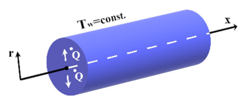
Figure 2.
Validation of numerical predictions for carrier liquid flow. D = 0.02 m; Tw = 293.15 K, q = −500 W.
Figure 2.
Validation of numerical predictions for carrier liquid flow. D = 0.02 m; Tw = 293.15 K, q = −500 W.
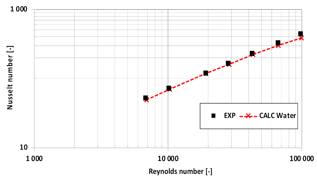
Figure 3.
(a) Comparison of assumed relative viscosity with experimental data of fine dispersive slurry for the Bingham model (Shook and Roco [6]; Slatter [82]). (b) Comparison of assumed relative yield stress with experimental data of fine dispersive slurry for the Bingham model (Shook and Roco [6]; Slatter [82]).
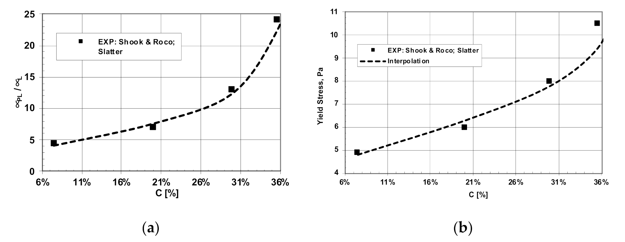
Figure 4.
(a) Comparison of temperature profiles for slurry and water; C = 30%, Ub = 3.50 m/s; q = −500 W/m. (b) Comparison of temperature profiles for slurry and water; C = 20%; Ub = 3.50 m/s; q = −500 W/m. (c) Comparison of temperature profiles for slurry and water; C = 10%; Ub = 3.50 m/s; q = −500 W/m. (d) Influence of solid concentration on the Nusselt number; Ub = 3.50 m/s; q = −500 W/m.
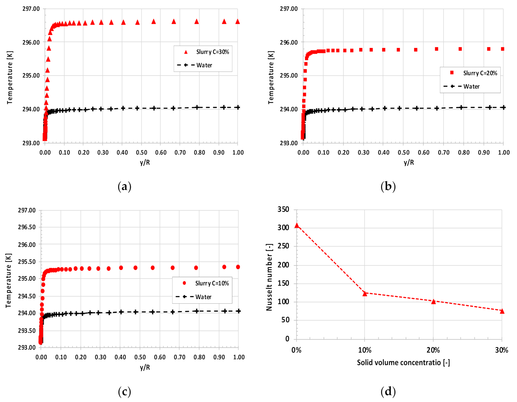
Figure 5.
(a) Comparison of velocity profiles for slurry and water; C = 30%; Ub = 3.5 m/s; q = −500 W/m. (b) Comparison of velocity profiles for slurry and water; C = 20%; Ub = 3.5 m/s; q = −500 W/m. (c) Comparison of velocity profiles for slurry and water; C = 10%; Ub = 3.50 m/s; q = −500 W/m; (d) Comparison of logarithmic profiles of dimensionless turbulent stresses for slurry and water; C = 30%; Ub = 3.50 m/s; q = −500 W/m.
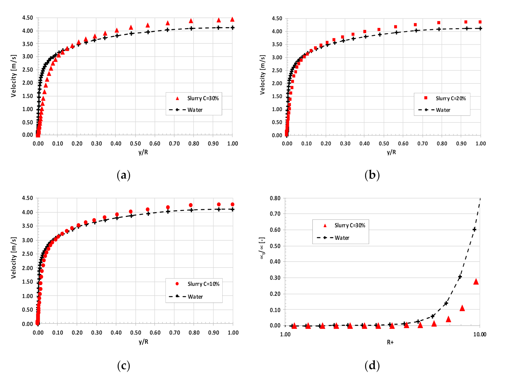
Figure 6.
(a) Influence of Reynolds number on the Nusselt number for fine dispersive slurry and water; (b) Influence of bulk velocity on the Nusselt number for fine dispersive slurry and water.
Figure 6.
(a) Influence of Reynolds number on the Nusselt number for fine dispersive slurry and water; (b) Influence of bulk velocity on the Nusselt number for fine dispersive slurry and water.
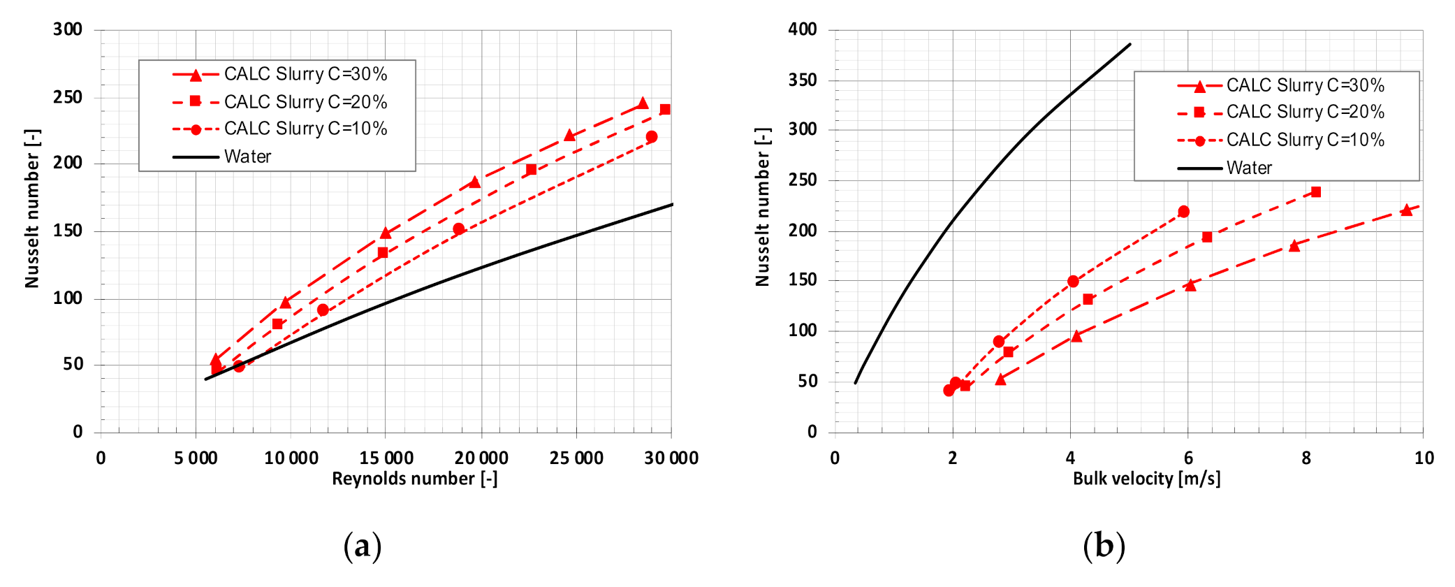
Figure 7.
New Nusselt number expressed by (42) versus the Nusselt number predicted by the mathematical model for C = 10%; 20% and 30%.
Figure 7.
New Nusselt number expressed by (42) versus the Nusselt number predicted by the mathematical model for C = 10%; 20% and 30%.

Table 1.
Parameters of the fine dispersive slurry for the Bingham model.
| Solid Volume Concentration | Bingham Model | |
|---|---|---|
| % | τo, Pa | μPL, Pa s |
| 10 | 5.10 | 0.004521 |
| 20 | 6.00 | 0.007032 |
| 30 | 8.00 | 0.013061 |
Table 2.
Thermal properties for limestone and liquid phase; D = 0.02 m; Tw = 293.15 K; q = −500 W/m.
Table 2.
Thermal properties for limestone and liquid phase; D = 0.02 m; Tw = 293.15 K; q = −500 W/m.
| Thermal Conduction for the Carrier Liquid | Thermal Conduction for Solid Particles | Specific Heat for the Carrier Liquid | Specific Heat for Solid Particles |
|---|---|---|---|
| W/(m K) | W/(m K) | J/(kg K) | J/(kg K) |
| 0.598 | 1.221 | 4183.00 | 795.00 |
Publisher’s Note: MDPI stays neutral with regard to jurisdictional claims in published maps and institutional affiliations. |
© 2021 by the author. Licensee MDPI, Basel, Switzerland. This article is an open access article distributed under the terms and conditions of the Creative Commons Attribution (CC BY) license (https://creativecommons.org/licenses/by/4.0/).
Share and Cite
MDPI and ACS Style
Bartosik, A. Numerical Modelling of Heat Transfer in Fine Dispersive Slurry Flow. Energies 2021, 14, 4909. https://doi.org/10.3390/en14164909
AMA Style
Bartosik A. Numerical Modelling of Heat Transfer in Fine Dispersive Slurry Flow. Energies. 2021; 14(16):4909. https://doi.org/10.3390/en14164909
Chicago/Turabian StyleBartosik, Artur. 2021. "Numerical Modelling of Heat Transfer in Fine Dispersive Slurry Flow" Energies 14, no. 16: 4909. https://doi.org/10.3390/en14164909
Note that from the first issue of 2016, this journal uses article numbers instead of page numbers. See further details here.