Aggregation of Radial Distribution System Bus with Volt-Var Control

Abstract

The high penetration of the distributed energy resources (DERs) encourages themselves to implement grid-supporting functions, such as volt-var control. The quasi-static time-series (QSTS) simulation is an essential technique to evaluate the impact of active DERs on the grid. Meanwhile, the increase of complexity on the circuit model causes a heavy computational burden of QSTS simulation. Although circuit reduction methods have been proposed, there have been few methods that can appropriately handle the distribution system (DS) with multiple voltage control devices, such as DERs implementing volt-var control. To address the remaining issues, this paper proposes an offline bus aggregation method for DS with volt-var control. The method determines the volt-var curve for the aggregated bus on the basis of historical data to reduce error in the aggregated model, and its offline process solves the computational convergence issue concerned in the online one. The effectiveness of the proposed method is validated in the simulation using a Japanese low-voltage DS model. The simulation results show that the proposed method can reduce the voltage error and computational time. Furthermore, the versatility of the proposed method is verified to show the performance does not heavily depend on how to select historical data for model-building.

1. Introduction

Continued cost reduction and policy support are driving the sustained uptake of wind power and solar photovoltaic (PV) across the world [1]. With the increased integration of the distributed energy resources (DERs) to power systems, the required capabilities of them have also changed. Earlier, it was required that DERs did not actively regulate voltage and shall trip on abnormal voltage/frequency [2]. Recently, requirements were revised so that they are capable of actively regulating voltage/frequency and shall ride through abnormal volt-age/frequency [3]. Such migration in the power system makes it challenging and important to understand the interaction between the power system and DERs.

In the DSs, many solutions have been proposed to mitigate the voltage rises, as well as to maximize the captured energy by the DERs. As solutions on the supply side, on-load tap changers (OLTCs) and their control schemes have been improved [4,5]. While on the demand side, various DER management methods are proposed [6,7]. Voltage-reactive power (volt-var) control by inverters of DERs is a reasonable solution to which DERs themselves, the cause of the issue, can contribute [8,9]. Since these methods will be eventually integrated to the same DS, coordinating them must be studied [10,11].

Quasi-static time-series (QSTS) analysis is essential to analyze the DSs with high penetrations of DERs for developing the above-mentioned solutions [12]. This solves a series of sequential steady-state power flow. Each time-step of the calculation is solved to rely on the information from the previous time-step solution [13]. Due to the features of QSTS analysis, as the number of buses, components, and a calculation time-step of the target circuit model increase, so does the accuracy and amount of available results. At the same time, it also increases the computational burden that makes it difficult to have enough case studies within a certain amount of time. Therefore, the simulation model used in the QSTS analysis should have as small a computational burden as possible while providing all the necessary results.

In order to reduce the computational burden of QSTS analysis, a fast power-flow calculation [14] and a machine learning-based approach [15] are proposed. Although they can reduce the computational burden and time, it is difficult to apply to the commercial software that offers fixed algorithms of power flow calculation, as well as a real-time simulation that cannot handle the original circuit model with a large number of nodes.

The circuit reduction algorithms are studied as other ways to reduce the computational burden. This is especially useful for a real-time simulation, including a hardware-in-the-loop (HIL) simulation, whose circuit models have the limitation of the number of nodes to run in real-time [16,17]. Although there have been proposed model reduction methods for dynamic analysis [18,19,20], these are not applicable to the QSTS analysis. Works focusing on circuit reduction of QSTS analysis using DS models have been reported in [17,21,22]. In these methods, the DERs are connected after feeder reduction, or the important buses, such as those with DERs, are preliminarily excluded from the reduction. Other circuit reduction approaches are proposed for the radial DSs in [23,24,25]. These approaches only focused on the fixed power factor control of DERs. Thus, they have not taken into account how to reduce buses with voltage control devices monitoring local voltages, such as DERs with volt-var control. In the DSs with many such voltage control devices, the gaps of the existing methods significantly reduce their usefulness.

The difficulty of this problem is how to represent the voltage behavior at the bus aggregated from multiple buses with voltage control devices. Recent studies [26,27] have proposed the bus aggregation with DER inverters implementing volt-var control, which monitors local voltage and adjusts reactive power output. These methods addressed the problem by modifying the volt-var control’s droop curve of the inverters at the aggregated bus from originally implemented ones. The authors in [26] periodically shifted the volt-var curve online in the QSTS procedure in order to reduce the bus voltage error between original and reduced networks. Although the frequent shift further reduced the error, it causes the power flow convergence issue that results in an increase in computational time. Meanwhile, the approach proposed in [27] determines the volt-var curve for the aggregated inverter offline on the basis of historical data. Although a small additional computational burden is required in the offline process, it is free from the power flow convergence issue. However, the effectiveness of the method has been validated using only limited specific daily PV and load data.

This paper is a further extension of the work in [27], and the main contributions are:

• To propose an offline bus aggregation method, which is free from the convergence problem, that can appropriately handle the DS models with many DERs implementing volt-var control and;
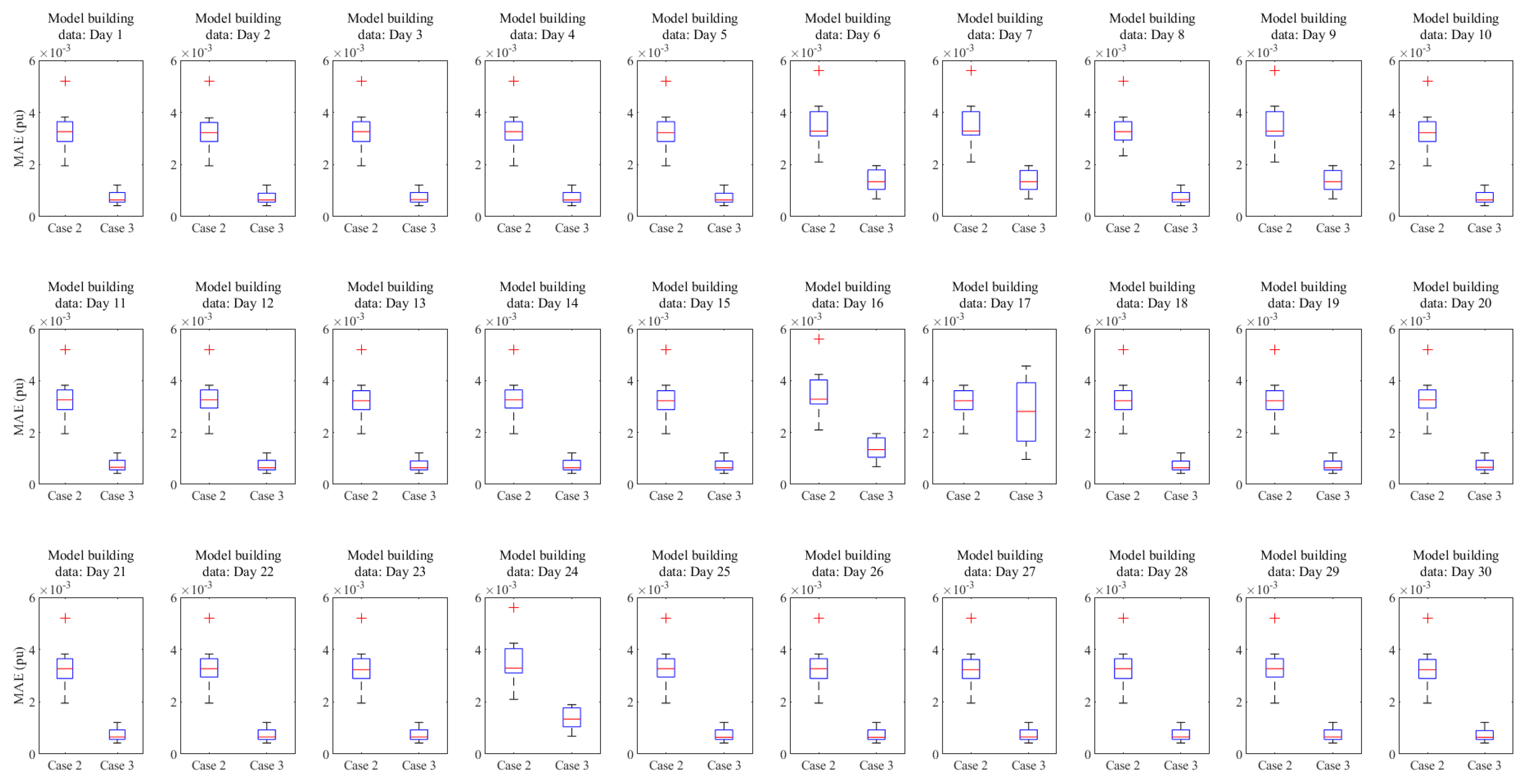
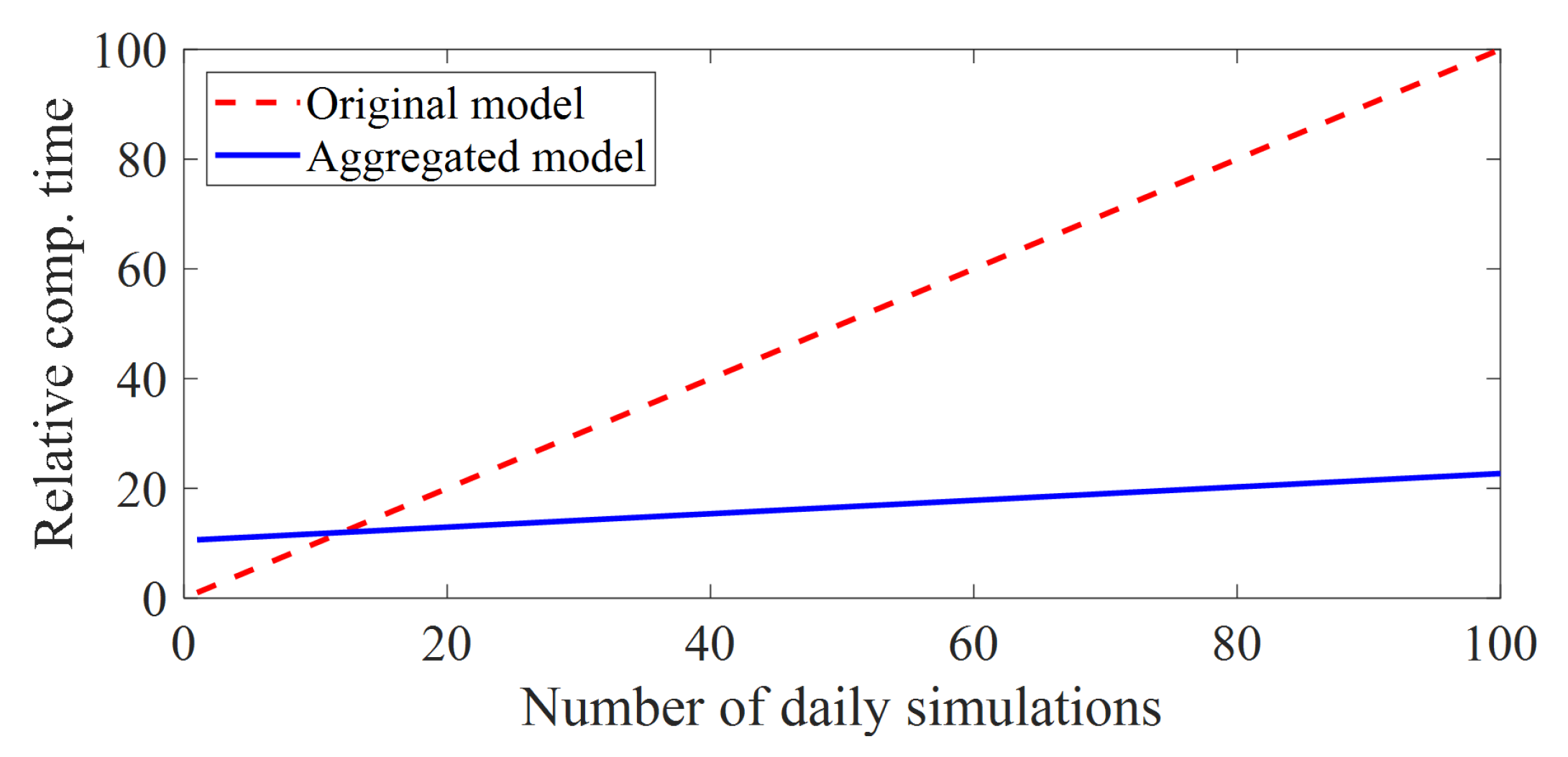
• To validate the effectiveness of the proposed method in terms of the voltage error and relative computational time as well as the versatility of the proposed method, that is, whether the aggregated model built by using historical data pertaining to a limited number of days is applicable to the rest of the days.

The remainder of the paper is organized as follows: Section 2 describes the procedure of the proposed bus aggregation method. The details about simulation studies and the obtained results are given in Section 3. Section 4 concludes the paper.

2. Aggregation of DS Buses with DERs Operationg with Volt-Var Control

This paper focuses on the bus aggregation to reduce the computational burden of QSTS analysis. The proposed method creates an aggregated DS model from an original one by aggregating any bus and the other subsequent buses to one bus. This approach is beneficial to consider, for example, coordination of an OLTC and numerous inverters, which operate with volt-var control, connected to subsequent buses and the monitoring of local voltages. Additionally, the proposed method is addressed to reduce the error due to the bus aggregation by determining a volt-var curve for the aggregated bus on the basis of historical data.

This section first describes a general circuit model to be aggregated. Then, the proposed bus aggregation approach is explained step-by-step, starting with the original full circuit model until the aggregated model.

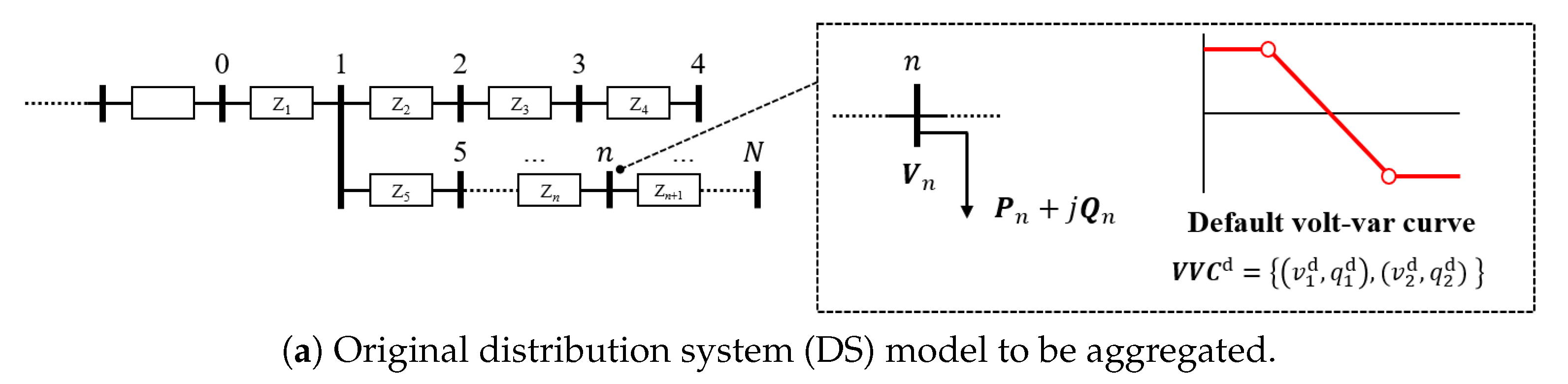
2.1. Original Circuit Model with Volt-Var Control

A part of the radial DS to be aggregated is shown in Figure 1a. Let $t\in \{1,\dots ,T\}$ be the time in simulation where T is the total simulation time, and $n\in \{0,1,\dots ,N\}$ be the index of the bus to be aggregated where N is the total number of them. Sequences of active power, reactive power, and voltage at bus n are represented by ${\mathit{P}}_n=(P_{t,n};t\in \{1,\dots ,T\})$, ${\mathit{Q}}_n=(Q_{t,n};t\in \{1,\dots ,T\})$, and ${\mathit{V}}_n=(V_{t,n};t\in \{1,\dots ,T\})$. Generally, the bus voltage ${\mathit{V}}_n$ can be calculated by the QSTS simulation when the active power ${\mathit{P}}_n$ and reactive power ${\mathit{Q}}_n$ are given. The active power ${\mathit{P}}_n$ and reactive power ${\mathit{Q}}_n$ can be divided into a passive part and active part, respectively, as follows:

$${\mathit{P}}_n={\mathit{P}}_n^{\mathrm{p}}+{\mathit{P}}_n^{\mathrm{a}},$$

(1)

$${\mathit{Q}}_n={\mathit{Q}}_n^{\mathrm{p}}+{\mathit{Q}}_n^{\mathrm{a}},$$

(2)

where superscripts $\mathrm{p}$ and $\mathrm{a}$ indicate a passive part and active part. The passive part represents the constant value, which is given time-series variation data in the simulation and does not depend on power flow results. Meanwhile, the active part consists of variable values depending on the power flow results given by

$${\mathit{P}}_n^{\mathrm{a}}=g_n\left({\mathit{x}}_n\right),$$

(3)

$${\mathit{Q}}_n^{\mathrm{a}}=f_n\left({\mathit{x}}_n\right),$$

(4)

where ${\mathit{x}}_n$ represents the input of control, such as local voltage and grid frequency, depending on the power flow results; and $g_n$ and $f_n$ indicate the functions of control algorithm of active parts of active power and reactive power. In the case of the volt-var control, the active part of reactive power is calculated in each time-step as follows:

$${\mathit{Q}}_n^{\mathrm{a}}=f^{\mathrm{vvc}}({\mathit{V}}_n,{\mathit{V}\mathit{V}\mathit{C}}_n),$$

(5)

where ${\mathit{V}\mathit{V}\mathit{C}}_n=\{(v_1,q_1),(v_2,q_2)\}$ indicates the volt-var curve at bus n, which can be defined by two points of voltage and a reactive power value set shown in Figure 1. $f^{\mathrm{vvc}}$ indicates the function of volt-var control, which derives a reactive power output when the volt-var curve and voltage are given. Here, the volt-var curve defined in IEC 61850-90-7 [28] is adopted. In the original model, we suppose that a reasonable default volt-var curve ${\mathit{V}\mathit{V}\mathit{C}}^{\mathrm{d}}=\{(v_1^{\mathrm{d}},q_1^{\mathrm{d}}),(v_2^{\mathrm{d}},q_2^{\mathrm{d}})\}$ for a distribution system operator (DSO) is set for all DERs.

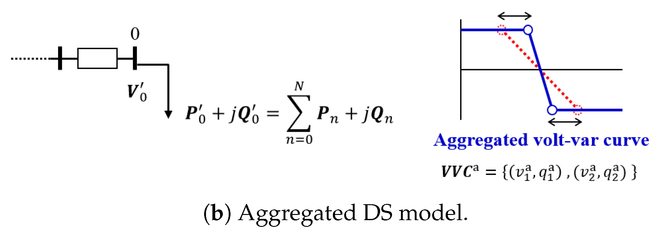
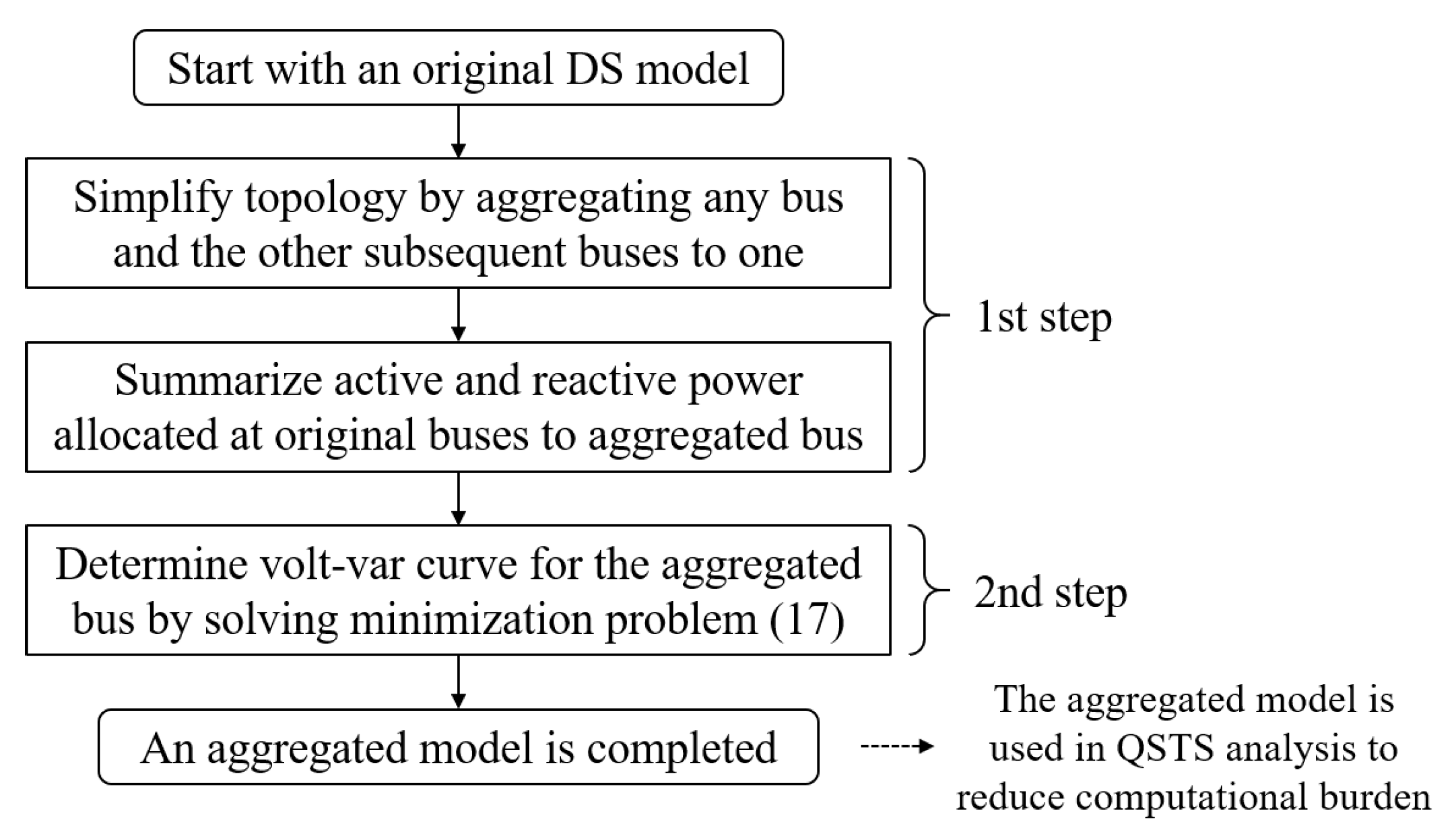
2.2. Bus Aggregation and Determination of Aggregated Volt-Var Curve

The flow of our proposed approach is shown in Figure 2. The approach can be divided into two major steps: aggregation of network topology and determination of the volt-var curve for the aggregated bus. These processes are supposed to be executed before main QSTS analysis to reduce its computational burden; that is, these are executed offline.

The first step is a straightforward aggregation to simplify the circuit topology. An arbitrary bus and the other subsequent buses in the original DS model are aggregated into one. In Figure 1, bus 0 is selected as an arbitrary bus, and buses 1 to N are aggregated into bus 0. The passive parts of active and reactive power, which should be given data in the simulation, at subsequent buses are also aggregated as follows:

$${{\mathit{P}}_0^{\mathrm{p}}}^{\prime }=\sum _{n=0}^N{\mathit{P}}_n^{\mathrm{p}},$$

(6)

$${{\mathit{Q}}_0^{\mathrm{p}}}^{\prime }=\sum _{n=0}^N{\mathit{Q}}_n^{\mathrm{p}},$$

(7)

where prime (${}^{\prime }$) represents the value of the aggregated model. Meanwhile, their active parts are represented by

$${{\mathit{P}}_0^{\mathrm{a}}}^{\prime }=g_n^{\prime }\left({\mathit{x}}_n\right),$$

(8)

$${{\mathit{Q}}_0^{\mathrm{a}}}^{\prime }=f_n^{\prime }\left({\mathit{x}}_n\right).$$

(9)

Replacing it with volt-var control, the active parts of them at bus 0 are represented by

$${{\mathit{P}}_0^{\mathrm{a}}}^{\prime }=0,$$

(10)

$${{\mathit{Q}}_0^{\mathrm{a}}}^{\prime }=f^{\mathrm{vvc}}({\mathit{V}}_0^{\prime },{\mathit{V}\mathit{V}\mathit{C}}^{\mathrm{a}}),$$

(11)

where ${\mathit{V}\mathit{V}\mathit{C}}^{\mathrm{a}}=(q_1^a,v_1^a),(q_2^a,v_2^a)$ represents the volt-var curve for the aggregated bus (hereinafter called aggregated volt-var curve). It is important to note that the active part of reactive power in the original model depends on each local bus voltage as shown in (5), while that in the aggregated model depends on the voltage at only bus 0, as shown in (11). Therefore, even if the default volt-var curve ${\mathit{V}\mathit{V}\mathit{C}}^{\mathrm{d}}$ at each bus in the original model is set to the same setting, it is not appropriate to use it as the aggregated volt-var curve ${\mathit{V}\mathit{V}\mathit{C}}^{\mathrm{a}}$. If they are not the same originally, ${\mathit{V}\mathit{V}\mathit{C}}^{\mathrm{d}}$ is still necessary to be given in the aggregated model. The solution to this issue is provided in the second step of the proposed method.

Here, the aggregation of apparent power should also be mentioned as a necessary perspective of bus aggregation with volt-var control. We let $S_n^{\mathrm{DER}}$ be the apparent power rating of the DER inverter at bus n, while that in the aggregated bus is the sum of them given by

$${S^{\mathrm{DER}}}^{\prime }=\sum _{n=0}^N{S}_n^{\mathrm{DER}}.$$

(12)

Let $P_{t,n}^{\mathrm{DER}}$ and $Q_{t,n}^{\mathrm{DER}}$ be the active and reactive powers of the DER inverter output in bus n at time t. Since there is a relation between apparent, active, and reactive powers of the DER inverter output as expressed in (13):

$$S_n^{\mathrm{DER}}\ge \sqrt{P_{t,n}^{{\mathrm{DER}}^2}+Q_{t,n}^{{\mathrm{DER}}^2}}.$$

(13)

This means that the apparent power rating is a constraint of the maximum reactive power output.

In the second step, which is our key approach, the volt-var curve for the aggregated bus is determined so that the aggregated bus voltage ${\mathit{V}}_0^{\prime }$ approximates the original one ${\mathit{V}}_0$ on the basis of historical data. Let ${\mathit{V}\mathit{V}\mathit{C}}^{\mathrm{a}}=(q_1^a,v_1^a),(q_2^a,v_2^a)$ be the volt-var curve for the aggregated bus (hereinafter called the aggregated volt-var curve), ${\mathit{P}}_n^{\mathrm{p}*}=({\mathit{P}}_{t,n}^{\mathrm{p}*};t\in \{1,\dots ,T\})$ and ${\mathit{Q}}_n^{\mathrm{p}*}=({\mathit{Q}}_{t,n}^{\mathrm{p}*};t\in \{1,\dots ,T\})$ be the historical data of passive parts of active and reactive powers at bus n, where the asterisk (*) indicates historical data. Suppose that the DERs with volt-var control are the only active devices in the circuit, and the active part of active power at bus n in the original model becomes ${\mathit{P}}_n^{\mathrm{a}*}=({\mathit{P}}_{t,n}^{\mathrm{a}*};t\in \{1,\dots ,T\})=\mathbf{0}$. Meanwhile, the historical sequences of the passive part of active, reactive powers, and active part of active power for the aggregated bus are derived as follows:

$${{{\mathit{P}}_0^{\mathrm{p}}}^{\prime }}^{*}=\sum _{n=0}^N{\mathit{P}}_n^{\mathrm{p}*},$$

(14)

$${{{\mathit{Q}}_0^{\mathrm{p}}}^{\prime }}^{*}=\sum _{n=0}^N{\mathit{Q}}_n^{\mathrm{p}*},$$

(15)

$${{{\mathit{P}}_0^{\mathrm{a}}}^{\prime }}^{*}=\sum _{n=0}^N{\mathit{P}}_n^{\mathrm{a}*}=\mathbf{0}.$$

(16)

To determine the aggregated volt-var curve ${\mathit{V}\mathit{V}\mathit{C}}^{\mathrm{a}}$ so that the voltage at bus 0 in the aggregated model ${\mathit{V}}_0^{\prime }$ approximates that in the original one ${\mathit{V}}_0$, the following minimization problem is solved:

$${\mathit{V}\mathit{V}\mathit{C}}^{\mathrm{a}}=\underset{\mathit{V}\mathit{V}\mathit{C}\in \mathbf{\psi }}{\mathrm{argmin}}\frac{1}{T}\sum _{t=1}^T|V_{t,0}({\mathit{P}}_n^{\mathrm{p}*},{\mathit{Q}}_n^{\mathrm{p}*},{\mathit{P}}_n^{\mathrm{a}*},{\mathit{V}\mathit{V}\mathit{C}}^{\mathrm{d}})-V_{t,0}^{\prime }({{{\mathit{P}}_0^{\mathrm{p}}}^{\prime }}^{*},{{{\mathit{Q}}_0^{\mathrm{p}}}^{\prime }}^{*},{{{\mathit{P}}_0^{\mathrm{a}}}^{\prime }}^{*},\mathit{V}\mathit{V}\mathit{C})|,$$

(17)

where $\mathbf{\psi }$ represents the set of volt-var curve candidates within the practical usage range. The voltage at bus 0 in the original model $V_{t,0}$ and that in the aggregated model $V_{t,0}^{\prime }$ can be derived by the power flow calculation when the historical data of active power, that of reactive power, and the volt-var curve setting for each model are given. The optimization problem can be solved by comparing the results of power flow calculation for all volt-var curve candidates $\mathit{V}\mathit{V}\mathit{C}\in$$\mathbf{\psi }$ of the aggregated model. Note that the mean absolute error (MAE) is adopted here, while other indices could be available depending on the purpose. Consequently, in the aggregated bus, the active part of reactive power is derived by (11) and (17).

3. Numerical Simulation

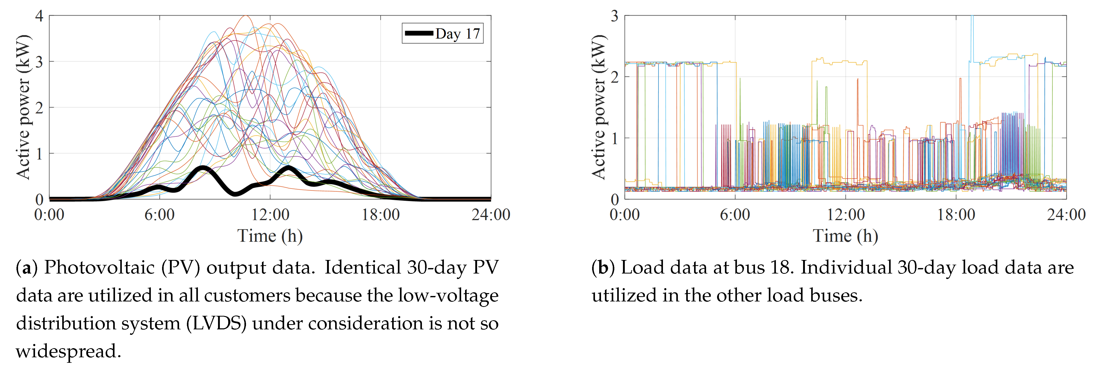
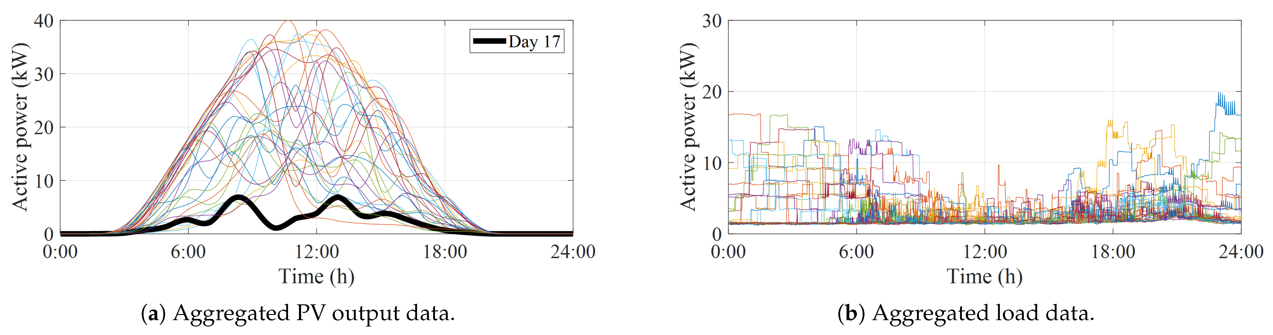
3.1. Simulation Outline

The numerical simulation is conducted to verify the effectiveness of the proposed method. The simulation models are developed in OpenDSS [29]. A Japanese general low-voltage distribution system (LVDS) model shown in Figure 3 is utilized for the simulation. The LVDS is a single-phase three-line system with 105 V and 210 V lines, thanks to the center-tapped secondary of the distribution transformer. Figure 3a,b shows the topology of original and aggregated LVDS models, respectively. In this simulation, the secondary side bus of the transformer (bus 0) and all subsequent buses (buses 1–18) are aggregated into one bus. The original model has 10 loads and PVs at buses 5–9 and 14–18. All PV inverters are equipped with volt-var control. The apparent power ratings of PV inverters are set 4.8 kW, which is 1.2 times that of PV panels. All PVs and loads are connected to the phase of 210 V, and the average of voltages in the two phases of 105 V is used for the evaluation.

The 30-day time-series data of PVs and loads with one-minute intervals, which are generated by the MATLAB application [30], are utilized in every single customer. Therefore, the total time-step T of daily simulation becomes 1440. The PV data in the original model are identical in all buses because the LVDS under consideration is not so widespread. Figure 4a shows the 30-day PV data of active power for all PV buses. Meanwhile, the individual load data are employed for each bus. Figure 4b shows the 30-day load data of active power at bus 18. Other 30-day load data for nine load buses are prepared as well. These net totals of PV and load data at each bus corresponds to the passive part of active power ${\mathit{P}}_n^{\mathrm{p}}$. That of reactive power ${\mathit{Q}}_n^{\mathrm{p}}$, the active part of active power ${\mathit{P}}_n^{\mathrm{a}}$ are set to zero. The 30-day load and PV data in the aggregated model derived on the basis of (6) are shown in Figure 5a,b, respectively. The net total of them similarly corresponds to the passive part of the active power at aggregated bus ${{\mathit{P}}_0^{\mathrm{p}}}^{\prime }$. The 30-day data are divided into one-day model-building data and 29-day validation data, and utilized in the case studies.

The aggregated volt-var curve ${\mathit{V}\mathit{V}\mathit{C}}^{\mathrm{a}}$ for the aggregated PV inverter at bus 0 is determined by solving (17). The one-day model-building data are utilized as the historical data of the passive part of active power ${\mathit{P}}_n^{\mathrm{p}*}$, ${{{\mathit{P}}_0^{\mathrm{p}}}^{\prime }}^{*}$. Note that the other historical data ${\mathit{Q}}_n^{\mathrm{p}*}$, ${\mathit{P}}_n^{\mathrm{a}*}$, ${{{\mathit{Q}}_0^{\mathrm{p}}}^{\prime }}^{*}$, ${{{\mathit{P}}_0^{\mathrm{a}}}^{\prime }}^{*}$ given in (17) is zero because the simulation focuses on the LVDS and volt-var control. As mentioned above, the default volt-var curve ${\mathit{V}\mathit{V}\mathit{C}}^{\mathrm{d}}$ given in (17) is assumed to be determined in a reasonable way. Here, it is determined in order to minimize the total difference between the voltages $V_{t,n}$ and $V^{\mathrm{ref}}$ as expressed in (18):

$${\mathit{V}\mathit{V}\mathit{C}}^{\mathrm{d}}=\underset{\mathit{V}\mathit{V}\mathit{C}\in \mathbf{\psi }}{\mathrm{argmin}}\sum _{n=0}^N\sum _{t=1}^T\{V_{t,n}({\mathit{P}}^{\mathrm{p}*},{\mathit{Q}}^{\mathrm{p}*},{\mathit{P}}^{\mathrm{a}*},\mathit{V}\mathit{V}\mathit{C})-V^{\mathrm{ref}}\},$$

(18)

where $V^{\mathrm{ref}}$ indicates the reference voltage. $V^{\mathrm{ref}}$ is assumed to be 101 V, where the median of the appropriate voltage range is in the Japanese LVDS. The Equation (18) can be solved by running the power flow calculation for the search range of $\mathit{V}\mathit{V}\mathit{C}$, that is, $\mathbf{\psi }$, as well as solving (17).

The proposed method is evaluated in terms of the accuracy and computational time. The aggregated model is built using one-day model-building data and evaluated by the other 29-day validation data. The evaluation in this manner is carried out for all combinations of thirty days, that is, aggregations based on thirty different model-building data were conducted.

3.2. Simulation Results

The effectiveness of the proposed method is evaluated by comparing the following three cases.

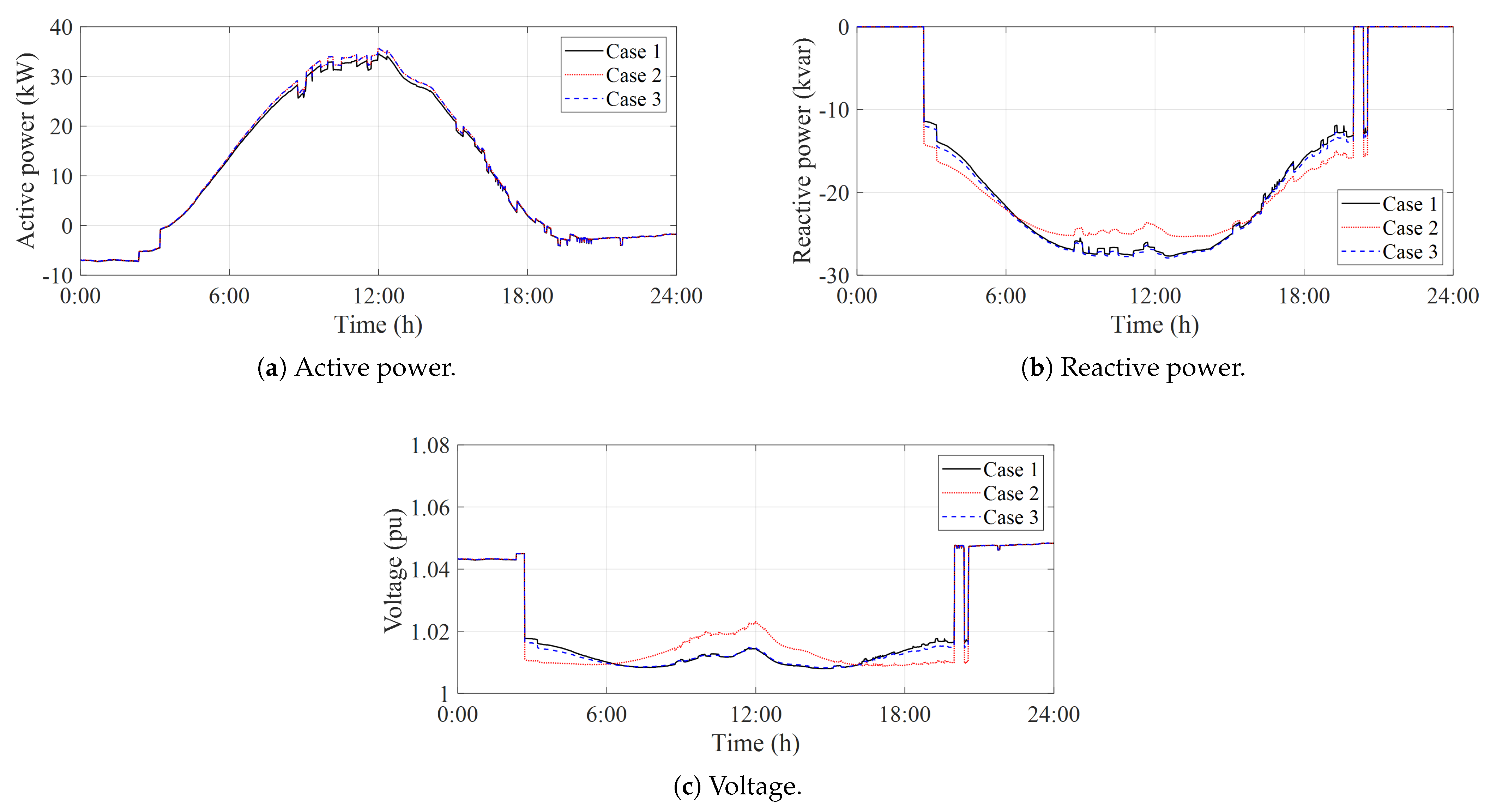
• Case 1: Original model with the default volt-var curve ${\mathit{V}\mathit{V}\mathit{C}}^{\mathrm{d}}$ on all PV inverters, that is, the original condition as a reference.
• Case 2: Aggregated model with the default volt-var curve ${\mathit{V}\mathit{V}\mathit{C}}^{\mathrm{d}}$ on aggregated PV at bus 0, that is, the conventional and straightforward aggregation method.
• Case 3: Aggregated model with the aggregated volt-var curve ${\mathit{V}\mathit{V}\mathit{C}}^{\mathrm{a}}$ on aggregated PV at bus 0, that is, our proposed aggregation method.

Table 1. MAEs of conventional (Case 2) and proposed (Case 3) methods over Case 1.

	Active Power (kW)	Reactive Power (kvar)	Voltage (pu)
Case 2	0.241	1.30	0.00330
Case 3	0.239	0.412	0.000891

shows the MAEs of daily active power, reactive power, and voltage at bus 0. The values show the MAEs of Case 2 and Case 3 over Case 1. These are averages of the daily MAE results for all case studies, that is, cases of all combinations to select model-building data. Furthermore, the randomly extracted daily profiles of each value are compared in Figure 6. Figure 6a shows there is no significant difference between three cases in the active power because the major thing that can make a difference is originally a small line loss.

In contrast, Case 2 of Table 1 and Figure 6a shows the reactive power has a much larger error over Case 1. The reason is activation of the volt-var control and its reactive power injection of PV inverters due to the voltage rise on their terminal. In the original model, farther inverters from bus 0 experience higher voltage rises and need to be compensated by absorbing reactive power. Meanwhile, in the aggregated model, an aggregated large PV is connected to bus 0 and experiences a smaller voltage rise.

Therefore, if the same volt-var curve ${\mathit{V}\mathit{V}\mathit{C}}^{\mathrm{d}}$ is implemented in both models, a mismatch occurs. When this is rectified by replacing ${\mathit{V}\mathit{V}\mathit{C}}^{\mathrm{d}}$ in an aggregated model with ${\mathit{V}\mathit{V}\mathit{C}}^{\mathrm{a}}$, it is observed that the results are explicitly close. The same discussion can be made for the voltage profile as there is a huge error, only when the PV generates, in Case 2 of Table 1 and Figure 6c, which is fixed with the use of ${\mathit{V}\mathit{V}\mathit{C}}^{\mathrm{a}}$. As a quantitative evaluation in Table 1, the MAEs of reactive power and voltage are reduced by 68.3% (1.30 to 0.412) and 73.0% (0.00330 to 0.000891), respectively, from Case 2 to Case 3.

Figure 7 shows ${\mathit{V}\mathit{V}\mathit{C}}^{\mathrm{d}}$, and the default volt-var curve determined for the original model, and ${\mathit{V}\mathit{V}\mathit{C}}^{\mathrm{a}}$, that is for the aggregated model in a case. It is found that the latter is narrower than the former. The trend is observed in the other cases. Since the aggregated model needs to represent all the PVs and loads in the LVDS, ${\mathit{V}\mathit{V}\mathit{C}}^{\mathrm{a}}$ shows the late operation of volt-var control and has a steeper curve. This suggests that it takes longer to start reactive power injection in the aggregated model, but it has a much quicker response to changes. This is reasonable, as it represents a collection of several PV inverters and their reaction.

Figure 8 shows the cross-validation results on all the combinations that select one-day model-building data and 29-day validation data from the 30-day data set. Each figure shows the boxplot of MAEs in voltages at bus 0 of case 2 and case 3, which are on the left and right side, respectively. On each box, the central mark indicates the median, and the bottom and top edges of the box indicate the 25th and 75th percentiles, respectively. The whiskers extend to the most extreme data points not considered outliers, and the outliers are plotted individually using the ‘+’ symbol. The outliers are values that are greater than $q_3+w\times (q_3-q_1)$ or less than $q_1-w\times (q_3-q_1)$, where w is the maximum whisker length 1.5, and $q_1$ and $q_3$ are the 25th and 75th percentiles of the sample data, respectively. The sample data here means validation results of every 29th day.

The validation results suggest the MAE in the voltage is explicitly reduced from Case 2 to Case 3 in each case except when Day 17 is used for the model-building data. The results suggest the proposed aggregation method is a robust scheme that can build the accurate aggregation model no matter what model-building data are given. The small amount of model-building data are also an advantage because it can reduce the computation time to build the aggregated model additionally required before the main QSTS simulation (see Figure 2). Although the results using Day 17 as model-building data are worse than the others, it reveals the data with small PV generation (see a bold profile in Figure 4a) should not be used as model-building data.

Finally, the proposed method is evaluated in terms of the calculation burden. Let the relative computational time required for daily QSTS simulation using the original model be 1, where that using the aggregated model is 0.1219. The computational times are average times of 2340 daily simulations in each model. The relative computational time using the aggregated model decreases by 88%. Meanwhile, the proposed method builds the aggregated model before the main QSTS simulation, therefore the additional computational time needs to be evaluated. Figure 9 shows the increase of relative computational time according to the number of daily QSTS simulations. The values are theoretical ones derived on the basis of each average computational time. The intercept of the aggregated model indicates the additional computational time for aggregation procedures. In this simulation, a daily QSTS simulation and 78 ones are carried out in the original and aggregated models, respectively, for solving (17), that is, the additional computational time becomes $1+(0.1219\times 78)=10.51$. As a result, the computational time of the aggregated model becomes shorter than that of the original model when the number of daily simulations is larger than 12.

4. Conclusions

This paper proposed a circuit reduction method in the DS with multiple volt-var control devices. While the penetration of DER with volt-var control has been increased, there have been few circuit reduction methods that can handle the DS model with such DERs implementing voltage control. Our proposed method aggregates an arbitrary bus and the other subsequent buses to one. The active power and reactive power at the original buses were also aggregated. Then, as a key point of our method, the volt-var curve for the aggregated bus was determined on the basis of the historical data so that the aggregated bus voltage behaves like that in the original model. Moreover, the proposed method is free from the computational convergence issue concerned in the online method because it is conducted offline.

The effectiveness of the proposed method was validated using the Japanese LVDS model. The aggregated model was built using one-day data and evaluated using the other 29-day data. To verify the versatility, that is, that the performance of the method does not heavily depend on how to choose model-building data, it was also evaluated when the other 29 days were respectively selected as the model-building data. The simulation results showed the proposed method reduces voltage error at the aggregated bus by 83% than the straightforward method. The results also showed the versatility of the proposed method. The most historical data excepting the day with low PV generation is applicable as the model-building data.

Meanwhile, in terms of the computational burden, the aggregated model built by the proposed method reduces the computational time required for the daily QSTS simulation by 88% compared to the original model. Although the proposed method needs additional computation before the main QSTS analysis, it was shown to be superior when the number of daily simulations exceeded 12. This superiority will become more prominent if the determination of the aggregated volt-var curve is sophisticated, which reduces the additional computational time for the aforementioned model aggregation.

The proposed method is beneficial to study coordination of the arbitrary bus and other subsequent buses with DERs that operate according to local voltages, for example, the coordination of an OLTC and multiple DERs with volt-var control. Although the method was validated by using the LVDS model and the implemented volt-var curve had no dead band, it can be applied to DS models with a larger number of buses and DERs implementing various volt-var curves. The offline nature of the method will become more effective in terms of reducing the computational burden when aggregating larger DS models. Meanwhile, aggregating larger models may require the option to maintain multiple critical buses. Therefore, future work should include validating the method when applied to larger DS models and selecting multiple critical buses to remain. The various volt-var curves also need to be considered.

References

1. IEA. World Energy Outlook 2018; IEA: Paris, France, 2018; Available online: https://www.iea.org/reports/world-energy-outlook-2018 (accessed on 1 June 2021).
2. IEEE Standard for Interconnecting Distributed Resources with Electric Power Systems; IEEE Std 1547-2003; IEEE: Piscataway, NJ, USA, 2003; pp. 1–28.
3. IEEE Standard for Interconnection and Interoperability of Distributed Energy Resources with Associated Electric Power Systems Interfaces; IEEE Std 1547-2018 (Revision of IEEE Std 1547-2003); IEEE: Piscataway, NJ, USA, 2018; pp. 1–138.
4. Akagi, S.; Takahashi, R.; Kaneko, A.; Ito, M.; Yoshinaga, J.; Hayashi, Y.; Asano, H.; Konda, H. Upgrading Voltage Control Method Based on Photovoltaic Penetration Rate. IEEE Trans. Smart Grid 2018, 9, 3994–4003. [Google Scholar] [CrossRef]
5. Kikusato, H.; Kobayashi, M.; Yoshinaga, J.; Fujimoto, Y.; Hayashi, Y.; Kusagawa, S.; Motegi, N. Coordinated voltage control of load tap changers in distribution networks with photovoltaic system. In Proceedings of the 2016 IEEE PES Innovative Smart Grid Technologies Conference Europe (ISGT-Europe), Ljubljana, Slovenia, 9–12 October 2016; pp. 1–6. [Google Scholar]
6. Zeraati, M.; Hamedani Golshan, M.E.; Guerrero, J.M. A Consensus-Based Cooperative Control of PEV Battery and PV Active Power Curtailment for Voltage Regulation in Distribution Networks. IEEE Trans. Smart Grid 2019, 10, 670–680. [Google Scholar] [CrossRef] [Green Version]
7. Kikusato, H.; Fujimoto, Y.; Hanada, S.; Isogawa, D.; Yoshizawa, S.; Ohashi, H.; Hayashi, Y. Electric Vehicle Charging Management Using Auction Mechanism for Reducing PV Curtailment in Distribution Systems. IEEE Trans. Sustain. Energy 2020, 10, 1394–1403. [Google Scholar] [CrossRef] [Green Version]
8. Smith, J.W.; Sunderman, W.; Dugan, R.; Seal, B. Smart inverter volt/var control functions for high penetration of PV on distribution systems. In Proceedings of the 2011 IEEE/PES Power Systems Conference and Exposition, Phoenix, AZ, USA, 20–23 March 2011; pp. 1–6. [Google Scholar]
9. Ustun, T.S.; Aoto, Y. Analysis of Smart Inverter’s Impact on the Distribution Network Operation. IEEE Access 2019, 7, 9790–9804. [Google Scholar] [CrossRef]
10. Ku, T.; Lin, C.; Chen, C.; Hsu, C. Coordination of Transformer On-Load Tap Changer and PV Smart Inverters for Voltage Control of Distribution Feeders. IEEE Trans. Ind. Appl. 2019, 55, 256–264. [Google Scholar] [CrossRef]
11. Fujimoto, Y.; Kikusato, H.; Yoshizawa, S.; Kawano, S.; Yoshida, A.; Wakao, S.; Murata, N.; Amano, Y.; Tanabe, S.; Hayashi, Y. Distributed Energy Management for Comprehensive Utilization of Residential Photovoltaic Outputs. IEEE Trans. Smart Grid 2018, 9, 1216–1227. [Google Scholar] [CrossRef]
12. IEEE Guide for Conducting Distribution Impact Studies for Distributed Resource Interconnection; IEEE Std 1547.7-2013; IEEE: Piscataway, NJ, USA, 2014; pp. 1–137.
13. Reno, M.J.; Deboever, J.; Mather, B. Motivation and requirements for quasi-static time series (QSTS) for distribution system analysis. In Proceedings of the 2017 IEEE Power & Energy Society General Meeting, Chicago, IL, USA, 16–20 July 2017; pp. 1–5. [Google Scholar]
14. Qureshi, M.U.; Grijalva, S.; Reno, M.J.; Deboever, J.; Zhang, X.; Broderick, R.J. A Fast Scalable Quasi-Static Time Series Analysis Method for PV Impact Studies Using Linear Sensitivity Model. IEEE Trans. Sustain. Energy 2018, 10, 301–310. [Google Scholar] [CrossRef]
15. Mahmoud, K.; Abdel-Nasser, M. Fast yet Accurate Energy-Loss-Assessment Approach for Analyzing/Sizing PV in Distribution Systems Using Machine Learning. IEEE Trans. Sustain. Energy 2019, 10, 1025–1033. [Google Scholar] [CrossRef]
16. Valdivia, V.; Gonzalez-Espin, F.; Diaz, D.; Foley, R. Low-frequency reduced-order modeling approach and implementation of grid emulation in hardware-in-the-loop platforms. In Proceedings of the 2015 17th European Conference on Power Electronics and Applications (EPE’15 ECCE-Europe), Geneva, Switzerland, 8–10 September 2015; pp. 1–7. [Google Scholar]
17. Nagarajan, A.; Nelson, A.; Prabakar, K.; Hoke, A.; Asano, M.; Ueda, R.; Nepal, S. Network reduction algorithm for developing distribution feeders for real-time simulators. In Proceedings of the 2017 IEEE Power & Energy Society General Meeting, Chicago, IL, USA, 16–20 July 2017; pp. 1–5. [Google Scholar]
18. Purba, V.; Johnson, B.B.; Jafarpour, S.; Bullo, F.; Dhople, S.V. Dynamic Aggregation of Grid-Tied Three-Phase Inverters. IEEE Trans. Power Syst. 2020, 35, 1520–1530. [Google Scholar] [CrossRef]
19. Leung, J.; Kinnaert, M.; Maun, J.C.; Villella, F. Model reduction in power systems using a structure-preserving balanced truncation approach. Electrric Power Syst. Res. 2020, 177, 106002. [Google Scholar] [CrossRef]
20. Zhu, Z.; Geng, G.; Jiang, Q. Power System Dynamic Model Reduction Based on Extended Krylov Subspace Method. IEEE Trans. Power Syst. 2016, 31, 4483–4494. [Google Scholar] [CrossRef]
21. Pecenak, Z.K.; Disfani, V.R.; Reno, M.J.; Kleissl, J. Multiphase Distribution Feeder Reduction. IEEE Trans. Power Syst. 2018, 33, 1320–1328. [Google Scholar] [CrossRef]
22. Pecenak, Z.K.; Disfani, V.R.; Reno, M.J.; Kleissl, J. Inversion Reduction Method for Real and Complex Distribution Feeder Models. IEEE Trans. Power Syst. 2019, 34, 1161–1170. [Google Scholar] [CrossRef]
23. Santos-Martin, D.; Lemon, S. Simplified Modeling of Low Voltage Distribution Networks for PV Voltage Impact Studies. IEEE Trans. Smart Grid 2016, 7, 1924–1931. [Google Scholar] [CrossRef]
24. Reiman, A.P.; McDermott, T.E.; Akcakaya, M.; Reed, G.F. Electric Power Distribution System Model Simplification Using Segment Substitution. IEEE Trans. Power Syst. 2018, 33, 2874–2881. [Google Scholar] [CrossRef]
25. Casolino, G.M.; Losi, A. Reduced Modeling of Unbalanced Radial Distribution Grids in Load Area Framework. IEEE Access 2020, 8, 179931–179941. [Google Scholar] [CrossRef]
26. Pecenak, Z.K.; Haghi, H.V.; Li, C.; Reno, M.J.; Disfani, V.R.; Kleissl, J. Aggregation of Voltage-Controlled Devices During Distribution Network Reduction. IEEE Trans. Smart Grid 2020, 12, 33–42. [Google Scholar] [CrossRef]
27. Kikusato, H.; Ustun, T.S.; Hashimoto, J.; Otani, K. Aggregate Modeling of Distribution System with Multiple Smart Inverters. In Proceedings of the 2019 International Conference on Smart Energy Systems and Technologies (SEST), Porto, Portugal, 9–11 September 2019; pp. 1–6. [Google Scholar]
28. IEC/TR 61850-90-7. Communication Networks and Systems for Power Utility Automation, Part 90-7: Object Models for Power Converters in Distributed Energy Resources (DER) Systems; International Electrotechnical Commission (IEC): Geneva, Switzerland, 2013. [Google Scholar]
29. Smith, J. Modeling High-Penetration PV for Distribution Interconnection Studies, Smart Inverter Function Modeling in OpenDSS, Rev. 2, 3002002271; Electric Power Research Institure (EPRI): Palo Alto, CA, USA, 2013; Available online: https://www.epri.com/research/products/000000003002002271 (accessed on 1 June 2021).
30. Brodén, D.A.; Paridari, K.; Nordström, L. Matlab applications to generate synthetic electricity load profiles of office buildings and detached houses. In Proceedings of the 2017 IEEE Innovative Smart Grid Technologies-Asia (ISGT-Asia), Auckland, New Zealand, 4–7 December 2017; pp. 1–6. [Google Scholar]
Figure 1. Schematic image of (a) original and (b) aggregated models. The proposed method aggregates an arbitrary bus (bus 0) and the other subsequent buses with active power and reactive power. Then, the volt-var curve for the aggregated bus is determined so that the voltage variations at bus 0 become similar.
Energies 14 05390 g001aEnergies 14 05390 g001b
Figure 2. Flow of proposed bus aggregation approach.
Energies 14 05390 g002
Figure 3. Simulation models of a Japanese LVDS. (a) The original model with 19 buses, including 10 PV and load buses, are (b) aggregated into one bus. Volt-var control is implemented in all PV inverters.
Energies 14 05390 g003
Figure 4. The 30-day time-series data in the original model. The net total of PV and load data at each bus corresponds to the passive part of active power P n p .
Energies 14 05390 g004
Figure 5. The 30-day time-series data in the aggregated model. The net total of them similarly corresponds to the passive part of the active power at aggregated bus P 0 p * . The profiles are derived on the basis of (6).
Energies 14 05390 g005
Figure 6. Profiles at bus 0 in original and aggregated models with volt-var control. These are randomly extracted one-day results of all case studies.
Energies 14 05390 g006
Figure 7. Volt-var curves determined in a case study. That for an aggregated bus V V C a is steeper than the default one V V C d . Similar trends are observed in the other cases.
Energies 14 05390 g007
Figure 8. Boxplot of mean absolute error (MAE) in the voltage of Case 2 (left bars) and Case 3 (right bar) over Case 1. The result of each case study, which uses each Day 1 to 30 as model-building data, is compared. The implementation of the proposed method (left bar to right bar) reduces the MAE in the voltage in almost all cases. The result whose model-building data are Day 17 reveals the PV profile with small generation (see Figure 4a) should not be used for the model-building data.
Energies 14 05390 g008
Figure 9. Relation between the number of daily simulations and relative computational time.
Energies 14 05390 g009