Configuring a UWB Based Location System for a UGV Operating in a Follow-Me Scenario

Abstract

Unmanned Ground Vehicles (UGV) are devices capable of performing basic working movements without the operator being in their immediate working environment. Their capabilities include but are not limited to the perception of the environment with the use of sensors, determining the platform’s position, and planning and executing its movement. Ultra Wideband (UWB) is one of the wireless communication technologies which is increasingly used in location systems. This article presents the use of UWB technology in developing a guide localization system for a UGV (one of the stages of implementing a follow-me system). The article describes tests carried out on the developed testbed. Their aim was to determine the hardware configuration of the anchor arrangement characterized by the minimum number of lost data packets during operation. In order to determine the influence of the analysed variables on the output values, the method of global sensitivity analysis for neural networks was used.

1. Introduction

The emerging challenges in transport, as well as the new tasks requiring an appropriate level of safety in systems supporting unmanned vehicle operators, require the use of the latest solutions and concepts, such as Unmanned Ground Vehicles (UGV) or unmanned aerial vehicles (UAVs) [1]. UGVs, depending on the application, can operate autonomously or be remotely controlled by the operator from the immediate vicinity of the platform or from a remote position outside of the working area.

Autonomous ground vehicles cover a broad range of technologies related to control. They include navigation systems, mission planning (which is related to object recognition), communication, algorithms for planning, learning, and analyzing data as well as Human Machine Interfaces (HMIs) [2].

The follow-me mode does not require such complex systems or manual control of the platform by the operator [3,4]. In this mode, the vehicle follows the route set by the guide. An important aspect of UGV navigation in the follow-me mode is the process of determining the exact location of the guide. Currently used approaches are distinguished based solely on on-board sensors, which include vision systems or lidars [5], stationary environmental features of the recognized environment, such as vision markers [6], or radio navigation signals [7]. For robots operating in a devastated environment, determining the exact location creates additional challenges. UGVs often use satellite navigation systems for both locating and autonomous navigation [8]. However, in many application areas, it is possible to navigate without the use of satellite systems. This applies to both emergency situations and natural disasters [9] as well as navigation in an industrial environment, which can include factory and warehouse halls [10]. There are many applications related to the use of odometry based on onboard sensors to accurately and reliably locate autonomously moving vehicles [5], although the greatest disadvantage of most existing wireless location solutions is their increasing location error [8]. One of the advantages of radio methods is that they are less sensitive to environmental conditions related to poor visibility caused by fog or smoke [11].

The first step in building a follow-me system is having the ability to determine the precise position of the guide in relation to the UGV. This is the premise for the study presented in the following paper, where this process forms a basis for the subsequent determination of the desired UGV trajectory [12]. A trajectory of the guide’s movement is generated that connects two or more of the guide’s locations. Then, the trajectory planning subsystem builds the path based on successive guide positions. The main task of the trajectory planning system is to generate input signals to the platform control system to ensure smooth movement of the UGV following the guide.

There are currently several technologies widely used to detect guides of certain environmental components, like laser, vision systems, ultrasound signals, GPS, and wireless technologies (like Bluetooth, Wi-Fi, etc.) [13,14]. Both vision systems and laser rangefinders are being used often because they offer additional functionalities regarding the observation of the UGV surroundings (with particular emphasis on the guide) [15,16]. Considering the case of working in an outdoor environment, vision systems are very susceptible to changing lighting conditions (mainly uneven lighting and poor visibility in dark conditions). On the other hand, laser rangefinders do not recognize environments in which there are transparent objects (e.g., glass) or dark surfaces and unfavorable weather conditions, such as snow or rain. On the other hand, ultrasonic sensors are sensitive to reflection phenomena and are susceptible to temperature changes, which may disrupt their proper operation [16]. Satellite navigation systems provide the determination of the absolute location of the receiver, but in turn are exposed to signal interference (electronic interference and jamming), the presence of multipath signals, and the presence of land covers (e.g., forest), which may make it impossible to detect desired locations [17]. In recent years, Ultra-Wideband (UWB) location systems have been gaining more and more popularity. These systems with high accuracy, down to single centimeters [18], are based on radio modules. In location systems that are based on UWB modules, the location of a mobile UWB node can be determined on the basis of measurements of the distance to UWB nodes located in known locations. UWB systems can be used in applications where the location accuracy of several dozen centimeters is sufficient instead of more complex and more expensive systems for determining the trajectory based on vision markers [19]. In addition, these units have a low power requirement, are resistant to radio interference (and do not interfere with most radio systems themselves), have high resistance to signal multiplication, both in LOS (Line of Sight) and NLOS (Non-Line) modes. of Sight), and the ability of signal propagation through objects [12,20].

In addition, the undoubted advantage of the UWB-based systems is a much larger area of their operation, because the latest solutions of the modules provide connectivity up to 60 m while ensuring the visibility of the antennas. The latest reports show studies that enable localization also outside the line of sight with similar accuracy [21]. Many studies have used UWB to locate certain nodes in sensor networks in the Internet of Things (IoT) environments [22] and detect moving robots or people indoors [23].

Locating objects based on UWB technology consists in sending very short data packets and uses radio energy scattering techniques (into frequency bands) with a very low power spectral density [24]. This provides the amount of bandwidth that allows large amounts of data to be transferred. The frequency ranges are used to ensure that UWB pulses can penetrate objects such as walls.

UWB technology also has several disadvantages. As these systems are low-power, their range is largely dependent on the type and number of objects in the environment. In addition, the location of UWB modules close to the conductor body is a factor that degrades accuracy and reduces range, because the human body consists mainly of water (which introduces additional electromagnetic wave scattering) [20,25].

Regardless of the presented limitations, UWB technology meets all the criteria for a guide’s detection system. Moreover, based on existing literature [15], it seems justified to base the operation of our system on UWB technology. We also wanted to use this opportunity to tackle some of the problems which may stem from the presented limitations. Many research questions in this area still remain open. This work is intended to complement the knowledge base in the field of UWB sensing, which has seen rapidly growing in the last few years.

2. Materials and Methods

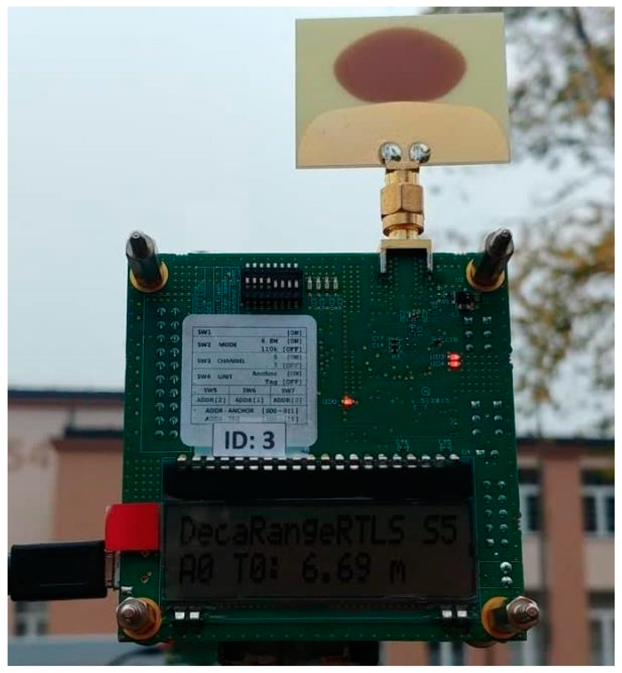
A UWB Decawave TREK 1000 is one of the available location systems on the market, and it was used in the research [26]. Mentioned system (Figure 1) allows the distance measurements between a portable transmitter called a tag and a receiver called an anchor. The discussed system consists of four anchors and one tag. The UWB modules use a two-way distance determination method which is called Two Way Ranging, and it is described schematically in Figure 2 [12].

The anchor–tag distance (between the anchor to the tag) can be calculated using the following mathematical formula:

$$\mathrm{d}=\mathrm{c}\left[\frac{\left({\mathrm{T}}_{\mathrm{RR}}-{\mathrm{T}}_{\mathrm{SP}}\right)-\left({\mathrm{T}}_{\mathrm{SR}}-{\mathrm{T}}_{\mathrm{RP}}\right)+\left({\mathrm{T}}_{\mathrm{RF}}-{\mathrm{T}}_{\mathrm{SR}}\right)-\left({\mathrm{T}}_{\mathrm{SF}}-{\mathrm{T}}_{\mathrm{RR}}\right)}{4}\right]$$

where c is the speed of light, T_SP, T_SR, and T_SF are the times of sending the polls and the packet responses by the anchor and the tag; and T_RP, T_RR, and T_RF are the times of receiving the polls and the packet responses by the anchor and the tag [12,27].

UWB modules can be described as wireless distance sensors. The refresh rate (3.57 Hz or 10 Hz) is dependent on the configuration of the module’s operational band (3.993 GHz or 6.489 GHz) [12].

The “Dromader” UGV (Figure 3a,b) was created at the Military University of Technology in Warsaw as part of the ICAR project (European Defence Agency). The anchors of the location system were placed on the UGV in the following configuration shown in Figure 3a,b. The present article is an extension of the research carried out in [12].

3. Configuring the UWB System

Conducted identification and simulation tests [4] have proven that it is possible to determine the position of a guide in a follow-me scenario and that this can be achieved using UWB technology. The next step in the process of developing a follow-me system was to determine the final hardware configuration, which would allow the minimization of data loss during wireless communication when the UGV is operational. Additionally, 4 UWB module configuration has possibilities for creating a follow-me solution [12].

This paper focuses on two placement configurations for the anchors (connected to the UGV). The first one, called the vertical configuration (Figure 3a), is a basic setup, which maximizes tag to anchor antenna visibility [4]. The second solution, called a spatial configuration (Figure 3b), is characterized by the distribution of anchors in a 3D space, as opposed to a planar placement from the vertical configuration. This solution is popular in >2 anchor configurations [12]. Spatial configuration provides more reliable data streams, which could be used to determine guide’s position. Because of this, the spatial configuration had been chosen for further development.

Because the UWB is capable of generating low-power radio signals, its range is limited in open environments. This poses an additional problem when taking the UGV into account. Not only spatial distribution on a ground-plane makes a difference in signal registration. The height on which the sensors are positioned on the UGV also plays a role in creating a robust and reliable guide detection system.

3.1. Testbed Setup

In order to conduct field tests, a special test site has been built in the Military University of Technology that spans 20 × 20 m². The selected UGV has been positioned on one of the edges of the site (Figure 4), and a special checkered net has been spun on it. The net consists of nodes 1 m apart from each other (Figure 5). The spatial configuration of 4 anchors has been deployed on the UGV (Figure 4), whereas the tag has been mounted on a tripod with the ability to be moved between nodes.

The test checkered net allows for fast redeployment of the tag when it’s time to reposition it during testing.

3.2. Testing Methodology

In order to assess the effectiveness of the spatial configuration, a series of data packets was registered. Each packet was set to last 30 s, during which data from four anchors (LF-left front, RF-right front, LB-left back, RB-right back) were recorded. The anchors were distributed as shown in Figure 6. Their vertical placement height was subjected to change during testing. A mobile tag was positioned in one of twelve test positions (T1–T12) shown in Figure 7, and its position’s height has also been subjected to change during testing. These changes represent the possibility for the guide to change elevation in relation to the UGV, similarly to when he would traverse an obstacle or a ditch. Additionally, the UGV was stationary during testing.

Registered data was later used in order to determine the data availability in the areas in front of the UGV. To do this, a percentage of lost data packets was calculated. These lost packets are symptoms of communication interference and breakdown. Since different UGVs may be used in follow-me scenarios, as mentioned before, the anchor’s vertical positions were changed during testing (configurations K1–K13,

Table 1. Anchor vertical placement in the UGV’s coordinate system.

Configuration	ZLF [m]	ZRF [m]	ZLB [m]	ZRB [m]
K1	1.12	1.12	1.12	1.12
K2	1.12	1.12	1.47	1.47
K3	1.12	1.12	1.82	1.82
K4	1.47	1.47	1.47	1.47
K5	1.47	1.47	1.82	1.82
K6	1.82	1.82	1.82	1.82
K7	1.47	1.47	1.12	1.12
K8	1.62	1.62	1.32	1.32
K9	1.62	1.62	1.82	1.82
K10	1.32	1.32	1.62	1.62
K11	1.82	1.82	1.62	1.62
K12	1.32	1.32	1.82	1.82
K13	1.82	1.82	1.32	1.32

). Additionally, each of the previously mentioned anchor positions has been tested, for each of the three tag position heights (H1–H3,

Table 2. Tag vertical placement in the UGV’s coordinate system.

Tag Height Name	Tag Height Value [m]
H1	0.6
H2	1.1
H3	1.6

). As it has been stated before, this parameter also influences the overall hardware system configuration for a follow-me scenario.

During testing, all data frames were registered for each of the four anchors for a set period. Based on that, the received data packet number (${\mathrm{l}}_{\mathrm{p}}$) was calculated for each anchor. In situations where at least one data frame was corrupted or incomplete, the entire packet was considered incomplete and was not calculated into the ${\mathrm{l}}_{\mathrm{p}}$ value. Additionally, knowing the period value and data rates of the anchors, the reference data packet number was calculated (${\mathrm{l}}_{\mathrm{r}}$) as follows:

$${\mathrm{l}}_{\mathrm{r}}=\mathrm{tf}$$

where t is record time (s) and f is sampling frequency (Hz).

The percentage of the correct sensor data packets (${\mathrm{l}}_{\%}$) was calculated using the following expression:

$${\mathrm{l}}_{\%}=\left(\frac{{\mathrm{l}}_{\mathrm{r}}-{\mathrm{l}}_{\mathrm{p}}}{{\mathrm{l}}_{\mathrm{r}}}\right)·100\%$$

where l_r is reference data packet number and l_p is received data packet number.

It has been assumed that in order to claim that a certain hardware configuration is usable for a follow-me scenario, the targeted minimum percentage of correct sensor data packets should be 90%. In further work, the percentage of correct sensor data ${\mathrm{l}}_{\%}$ has been substituted with a percentage of lost data packets P:

$$\mathrm{P}=100\%-{\mathrm{l}}_{\%}$$

where l_% is the percentage number of correct distance measurements.

Anchors were paired together into two groups: forward group and back group. Anchor height changes were done in said pairs, so that during reconfiguration two anchors always moved vertically. Height values represent the geometrical center point of each anchor’s antenna. Tag positions were labeled X_tag, Y_tag, Z_tag, and the percentage of lost data packets for each of the anchor were labeled LF, RF, LB, RB.

In conclusion, during testing a dataset containing 456 records was created, representing the LF, RF, LB, and RB values for each of the tag positions and height in relation to each of the anchor positions. The mentioned dataset includes the following records (variables):

• H_front—height of the front anchors in relation to ground plane (H_front = Z_LF = Z_RF),
• H_back—height of the back anchors in relation to ground plane (H_back = Z_LB = Z_RB),
• X_tag—position of the geometric center of the tag’s antenna cast on the x axis of the UGV’s coordinate system,
• Y_tag—position of the geometric center of the tag’s antenna cast on the y axis of the UGV’s coordinate system,
• H_tag—position of the geometric center of the tag’s antenna cast on the z axis of the UGV’s coordinate system,
• LF—percentage of lost data packets for the left-front anchor,
• RF—percentage of lost data packets for the right-front anchor,
• LB—percentage of lost data packets for the left-back anchor,
• RB—percentage of lost data packets for the right-back anchor.

Table 1, Table 2 and

Table 3. Tag positions in the UGV’s coordinate system.

Position	Xtag [m]	Ytag [m]	Ztag [m]
T1	−5	5	H1,H2,H3
T2	0	5	H1,H2,H3
T3	5	5	H1,H2,H3
T4	−5	10	H1,H2,H3
T5	0	10	H1,H2,H3
T6	5	10	H1,H2,H3
T7	−5	15	H1,H2,H3
T8	0	15	H1,H2,H3
T9	5	15	H1,H2,H3
T10	−5	20	H1,H2,H3
T11	0	20	H1,H2,H3
T12	5	20	H1,H2,H3

present values for each of the changed parameters. Table 1 shows data regarding anchor vertical positions. Table 2 shows data regarding tag vertical positions. Table 3 shows tag positions in the UGV’s coordinate system.

During testing, data packets were recorded using a laptop with a Matlab/Simulink suite.

• Testing procedure included the following steps:
• Setting up anchor positions to K1;
• Setting up tag height to H1;
• Setting up tag position to T1;
• Registering data packets;
• Moving tag position to T2;
• Registering data packets;
• Repeating steps 5 and 6 until reaching the T12 position;
• Changing tag height to H2;
• Repeating steps from 2 to 7;
• Changing tag height to H3;
• Repeating steps from 2 to 7;
• Changing anchor positions from K2 to K13 repeating steps from 2 to 11 each time.

4. Configuration Results

Results from testing on the number of data packets lost are shown in Figure 8. Figure 9 shows the average value of data packets lost for each configuration (the value was calculated from a series of 36 tests).

The average values of the number of data packets lost show that configurations no. 3, 8, and 9 (Figure 9) do not meet the set up requirement of 10% possible data packets lost, thus rendering them unusable for further testing and analysis. Removing these configurations allows for a more precise data analysis. Figure 10 and Figure 11 show the same data types as Figure 8 and Figure 9, but without said configurations.

Further analysis of registered data saw a histogram breakdown of variables LF, RF, LB, and RB (Figure 12). In all cases, a larger count correlates with a set of lower amounts of data packets lost.

Table 4. Basic statistical values of variables LF, RF, LB, RB.

Variable	Arithmetic Mean Value [%]	Minimum [%]	Maximum [%]	Standard Deviation [%]
LF	0.51	0	8.00	0.70
RF	0.42	0	5.50	0.57
LB	0.59	0	6.83	0.82
RB	0.84	0	7.33	1.10

shows statistical values of registered LF, RF, LB, and RB values. Their averages are less than 1% and the maximum values don’t exceed 8%. In each case, the standard deviation is greater than the arithmetic mean value but is less than twice the arithmetic mean value.

Figure 13, Figure 14 and Figure 15 show the consecutive dotted graphs of relations between variables LF, RF, LB, RB, and coordinates X_tag, Y_tag, and Z_tag.

Because of the discrete nature of the dataset as well as the limited volume of data points, it was impossible to use approximation methods to plot correlations between (a) LF, (b) RF, (c) LB, and (d) RB values and X_tag, Y_tag, Z_tag coordinates. Because of this, a method of global sensitivity analysis for neural networks was employed.

5. Global Sensitivity Analysis

The global sensitivity analysis module was implemented using the Statistica environment and was based on a data model described with the use of neural networks. This is further supported by the ability to design and train neural networks using the Statistica Automatic Neural Networks (SANN) module [27,28].

The global sensitivity analysis method allows determining the importance of individual input variables in the neural network [28]. It works by examining the prediction error of a trained neural network when for each mentioned input its values are changed with their arithmetic average (obtained from the training set). This method stops the input variables from providing new information to the neural network, which may cause the change of the final prediction error. It also shows that the trained neural network is characterized by a specified sensitivity to each input variable. Every trained neural network is then characterized by a variable illustrating the increase in error after removal of a certain input variable (the quotient of the network error without an individual variable to the error with a full set of inputs) is calculated. If the aforementioned value is less than or equal to 1, the analysis input variable can be permanently removed without the loss of quality of the neural network [28].

The global sensitivity analysis method is not free from limitations. For a given data set, global sensitivity analysis is not a universal method, i.e., the obtained results refer only to the created neural network. This is due to the fact that the analyzed variables can be correlated with each other, while the multitude of parameters of the neural network, i.e., the number of neurons in the layers, teaching algorithms, and the method of initializing the input weights of the neural network generate a variety of results of the global sensitivity analysis. For these reasons, conclusions should not be drawn from a single neural network. Performing the sensitivity analysis for a series of neural models and the obtained reproducibility of the results provide the necessary basis for the possibility of determining conclusions about the importance of each of the analyzed variables.

In order to prepare a global sensitivity analysis using the Statistica software, it was required to create a neural network model describing the data set. The first stage of building a neural model is the division of variables into inputs and outputs. Therefore, the nine described variables were divided into five input variables: H_front, H_back, X_tag, Y_tag, and H_tag, and four output variables: LF, RF, LB, and RB.

The next step saw the determination of the number of samples in random data. The training set contained the input data (H_front, H_back, X_tag, Y_tag, and H_tag) and associated responses (LF, RF, LB, and RB). It was then divided into three parts in order to train the network with the use of the learning algorithm, test set, and validation set.

The validation set carried out periodical validation during the training process in order to prevent the overlearning phenomenon, while the test set was intended for the final verification of the results of the neural network (checking if the network can generalize the results). The discussed sets were selected randomly, but their number was adopted as follows: the training set consisted of 60% of the original data set, the validation set consisted of 20% of the original data set, and the test set also consisted of 20% of the original data set.

Further work saw the construction of an MLP neural network with one hidden layer. To determine the number of neurons in the hidden layer and the activation function of the neural network in the hidden and output layers, it was assumed that the number of neurons should be within the range (25,50), while in the case of the activation function, the functions available in the software were selected, including linear, logistic, exponential, and hyperbolic tangent functions. Then, the SANN created and taught 5000 neural networks from which 100 of the best variants were selected for further analysis. Examples of those networks are presented in

Table 5. Examples of a teaching process of selected neural networks.

Netw. ID	Network Name	Quality (Teaching)	Quality (Testing)	Quality (Valid.)	Error (Teaching)	Error (Test)	Error (Valid.)	Activ. Function (Hidden Layer)	Activ. Function (Output Layer)
1	MLP 5-49-4	0.85	0.75	0.99	3.49	5.56	1.87	Log.	Exp.
2	MLP 5-32-4	0.99	0.95	0.99	0.13	1.11	0.09	Tanh.	Log.
7	MLP 5-35-4	0.83	0.79	0.99	3.80	4.68	0.06	Log.	Log.
8	MLP 5-35-4	0.94	0.76	0.99	1.27	5.86	0.18	Tanh.	Log.
13	MLP 5-36-4	0.92	0.83	0.99	1.71	3.93	0.05	Tanh.	Log.
18	MLP 5-25-4	0.97	0.94	0.99	0.65	1.42	0.07	Tanh.	Log.
23	MLP 5-38-4	0.85	0.75	0.99	3.51	5.61	0.98	Log.	Exp.
24	MLP 5-29-4	0.95	0.82	0.99	1.04	4.27	1.27	Tanh.	Log.
48	MLP 5-28-4	0.83	0.78	0.99	3.81	5.10	0.06	Log.	Log.
49	MLP 5-45-4	0.85	0.80	0.99	3.48	4.61	0.02	Tanh.	Log.
57	MLP 5-25-4	0.98	0.95	0.99	0.30	1.01	0.06	Log.	Log.
73	MLP 5-42-4	0.84	0.79	0.99	3.60	4.91	0.13	Log.	Log.
78	MLP 5-25-4	0.95	0.87	0.99	1.11	3.13	0.07	Log.	Log.
79	MLP 5-36-4	0.84	0.79	0.99	3.58	4.76	0.19	Tanh.	Log.
90	MLP 5-35-4	0.99	0.96	0.99	0.11	1.16	0.20	Tanh.	Log.

.

The neural networks’ teaching results have been shown in Table 5. These values indicate a large diversity in results among the network quality values: 0.83–0.99 (learning), 0.75–0.96 (testing); error values: 0.10–3.81 (learning), 1.01–5.86 (testing), 0.02–1.27 (validation); and the number of neurons in the hidden layer: 25–49. The logistic function (Log.), the hyperbolic tangent (Tanh.), and exponential function (Exp.) were used in the neural network teaching activation functions (Table 5). All presented neural networks are characterized by a high value of validation quality equal to 0.99. The error function is the sum of squares (SOS) between the setpoints and the output values from the neural network. The results of global sensitivity analysis for selected neural network models are presented in

Table 6. The results of global sensitivity analysis for selected 15 neural network models.

Network Name	Global Sensitivity Analysis
	Hfront	Hback	Xtag	Ytag	Htag
2. MLP 5-32-4	29.11	21.36	14.35	3.78	1.89
18. MLP 5-25-4	15.18	14.93	8.11	2.14	1.05
24. MLP 5-29-4	6.07	6.30	4.01	1.40	0.76
29. MLP 5-29-4	21.98	16.38	11.08	2.72	1.33
33. MLP 5-38-4	12.47	11.51	5.99	1.95	1.24
34. MLP 5-41-4	7.01	6.96	4.51	1.31	0.84
38. MLP 5-31-4	12.56	5.85	4.08	1.78	1.15
41. MLP 5-29-4	8.95	5.88	4.59	1.55	1.10
45. MLP 5-40-4	6.50	5.11	4.79	1.40	0.84
57. MLP 5-25-4	26.73	25.44	16.56	3.08	1.39
63. MLP 5-27-4	26.79	12.83	9.00	2.16	2.09
64. MLP 5-33-4	20.96	8.20	5.82	1.97	1.08
69. MLP 5-37-4	20.83	9.62	6.09	2.23	1.03
76. MLP 5-26-4	9.77	7.46	5.86	1.38	0.97
89. MLP 5-45-4	18.33	17.50	8.50	2.57	1.38
90. MLP 5-35-4	30.42	20.87	17.77	3.72	2.19
Arithmetic average	17.11	12.26	8.19	2.20	1.27

.

The above results show that none of the analyzed variables obtained the mean value lower than 1, which indicates a significant impact of each of them on the input variables. The variables most strongly influencing the output variables are H_front (17.11) and H_back (12.26). The remaining variables achieved the following results: X_tag (8.19), Y_tag (2.20), and H_tag (1.27). Global sensitivity analysis proves the relevance of the mentioned variables in configuring a UWB based location system.

6. Summary

The experimental research has shown that the average value of the percentage of lost data packages for the front anchors was less than 8%, and about 10% for the rear anchors, which translates into the percentage of the average number of correct measurements equal to 92% for the front anchors and 90% for the rear anchors. This proves that within the 4 UWB module configurations which had been looked into there are possibilities for creating a follow-me solution. The positioning of anchors on the UGV plays a significant role in the effectiveness of the developed solution, as seen in configurations K3, K8, and K9, which have exceeded the maximum amount of data packets lost for a follow-me system. When looking into the average amount of data packets lost, it is possible to pick configuration K11 as the one having the lowest value of the said parameter.

Conducted global sensitivity analysis has shown that all analyzed input variables play an important role in this setup and that none of them can be removed without impacting the effectiveness of the guide detection component. The height of the front and rear anchors in relation to the ground seems to have the greatest impact on the amount of data packets lost in UWB wireless communication in the considered measurement variant of the UGV. Next in line of importance is the X_tag variable, which has a greater impact on communication stability in the UWB wireless communication than Y_tag. This is due to hindered propagation of the radio signals in the extreme tag positions (T1,T3, etc.). Tag height relative to the ground has the least impact on the number of packet losses in wireless UWB communication, which bodes well for using this technology in unstructured terrain.

In summary, the proposed testing methodology as well as achieved results allowed the research team to determine the desired hardware configuration for a UWB guide detection system that would be used in a follow-me scenario alongside the “Dromader” UGV.

Moving on with the development of a follow-me system, a set of functionalities will have to be developed. One of them would be safety functions influencing the UGV’s engine, hydraulic drive pumps, and turn actuators. This is crucial, as the currently developed solution interprets drops in the guide’s position as simple data loss. Considering that the UGV in question is weighing hundreds of kilograms and can generate large amounts of torque, it needs to be strictly managed. Employing the system of system’s approach, the team has decided that the so called “safety layer” will not be a part of the guide’s detection system but instead will be a separate entity within the system, as the team is looking into other sensor types to be injected into the follow-me system.

Future work on the follow-me system will focus on developing both the mentioned safety layer as well as the low-level UGV layer, to allow the UGV to drive itself.

References

- Galar, D.; Kumar, U.; Senevirante, D. Robots, Drones, UAVs and UGVs for Operation and Maintenance; CRC Press, Taylor & Francis Group: Boca Raton, FL, USA, 2020. [Google Scholar]
- Ivanova, K.; Gallasch, G.E.; Jordans, J. Automated and Autonomous Systems for Combat Service Support: Scoping Study and Technology Prioritization; Defence Science and Technology Group Edinburgh SA Australia, Australian Government, Department of Defense: Edinburgh, Australia, 2016. Available online: https://www.dst.defence.gov.au/sites/default/files/publications/documents/DST-Group-TN-1573.pdf (accessed on 10 June 2021).
- Meet Burro. Available online: https://www.augeanrobotics.com (accessed on 10 June 2021).
- Malon, K.; Łopatka, J.; Rykala, Ł.; Łopatka, M. Accuracy Analysis of UWB Based Tracking System for Unmanned Ground Vehicles. In Proceedings of the 2018 New Trends in Signal Processing (NTSP), Demänovská Dolina, Slovakia, 10–12 October 2018; pp. 1–7. [Google Scholar]
- Qingqing, L.; Queralta, J.P.; Gia, T.N.; Tenhunen, H.; Zou, Z.; Westerlund, T. Visual odometry offloading in Internet of vehicles with compression at the edge of the network. In Proceedings of the 2019 Twelfth International Conference on Mobile Computing and Ubiquitous Network (ICMU), Kathmandu, Nepal, 4–6 November 2019; pp. 1–2. [Google Scholar]
- Kong, W.; Zhang, D.; Wang, X.; Xian, Z.; Zhang, J. Autonomous landing of an UAV with a ground-based actuated infrared stereo vision system. In Proceedings of the 2013 IEEE/RSJ International Conference on Intelligent Robots and Systems, Tokyo, Japan, 3–7 November 2013; pp. 2963–2970. [Google Scholar]
- Faragher, R.; Harle, R. An analysis of the accuracy of bluetooth low energy for indoor positioning applications. In Proceedings of the 27th International Technical Meeting of The Satellite Division of the Institute of Navigation (ION GNSS+ 2014), Tampa, FL, USA, 8–12 September 2014; pp. 201–210. [Google Scholar]
- Stempfhuber, W.; Buchholz, M. A precise, low-cost RTK GNSS system for UAV applications. In Proceedings of the Unmanned Aerial Vehicle in Geomatics (ISPRS), Zurich, Switzerland, 14–16 September 2011; pp. 289–293. [Google Scholar]
- Cui, J.Q.; Phang, S.K.; Ang, K.Z.; Wang, F.; Dong, X.; Ke, Y.; Chen, B.M. Drones for cooperative search and rescue in post-disaster situation. In Proceedings of the 2015 IEEE 7th International Conference on Cybernetics and Intelligent Systems (CIS) and IEEE Conference on Robotics, Automation and Mechatronics (RAM), Siem Reap, Cambodia, 15–17 July 2015; pp. 167–174. [Google Scholar]
- Tiemann, J.; Wietfeld, C. Scalable and precise multi-UAV indoor navigation using TDOA-based UWB localization. In Proceedings of the 2017 International Conference on Indoor Positioning and Indoor Navigation, Sapporo, Japan, 18–21 September 2017; pp. 1–7. [Google Scholar]
- Hightower, J.; Borriello, G. Location systems for ubiquitous computing. IEEE Comput. 2001, 34, 57–66. [Google Scholar] [CrossRef] [Green Version]
- Rykała, Ł.; Typiak, A.; Typiak, R. Research on Developing an Outdoor Location System Based on the Ultra-Wideband Technology. Sensors 2020, 20, 6171. [Google Scholar] [CrossRef] [PubMed]
- Cifuentes, C.A.; Frizera, A.; Carelli, R.; Bastos, T. Human–robot interaction based on wearable IMU sensor and laser range finder. Robot. Auton. Syst. 2014, 62, 1425–1439. [Google Scholar] [CrossRef]
- Germa, T.; Lerasle, F.; Ouadah, N.; Cadenat, V. Vision and RFID data fusion for tracking people in crowds by a mobile robot. Comput. Vis. Image Underst. 2010, 114, 641–651. [Google Scholar] [CrossRef]
- Guevara, A.E.; Hoak, A.; Bernal, J.T.; Medeiros, H. Vision-based self-contained target following robot using bayesian data fusion. In Proceedings of the International Symposium on Visual Computing, Las Vegas, NV, USA, 12–14 December 2016; pp. 846–857. [Google Scholar]
- Peng, W.; Wang, J.; Chen, W. Tracking control of human-following robot with sonar sensors. In Proceedings of the International Conference on Intelligent Autonomous Systems, Shanghai, China, 3–7 July 2016; pp. 301–313. [Google Scholar]
- GPS: Emerging Trends. Available online: https://www.imua.org/Files/reports/999110.html (accessed on 10 June 2021).
- Peña Queralta, J.; Martínez Almansa, C.; Schiano, F.; Floreano, D.; Westerlund, T. UWB-based system for UAV Localization in GNSS-Denied Environments: Characterization and Dataset. In Proceedings of the 2020 IEEE/RSJ International Conference on Intelligent Robots and Systems (IROS), Las Vegas, NV, USA, 25–29 October 2020; pp. 4521–4528. [Google Scholar]
- Furtado, J.S.; Liu, H.H.; Lai, G.; Lacheray, H.; Desouza-Coelho, J. Comparative analysis of optitrack motion capture systems. In Advances in Motion Sensing and Control for Robotic Applications; Springer: Heidelberg, Germany, 2019; pp. 15–31. [Google Scholar]
- Alarifi, A.; Al-Salman, A.; Alsaleh, M.; Alnafessah, A.; Al-Hadhrami, S.; Al-Ammar, M.A.; Al-Khalifa, H.S. Ultra-Wideband indoor positioning technologies: Analysis and recent advances. Sensors 2016, 16, 707. [Google Scholar] [CrossRef]
- Prorok, A.; Tomé, P.; Martinoli, A. Accommodation of NLOS for Ultra-Wideband TDOA localization in single-and multi-robot systems. In Proceedings of the 2011 International Conference on Indoor Positioning and Indoor Navigation, Guimarães, Portugal, 21–23 September 2011; pp. 1–9. [Google Scholar]
- Chen, Y.C.; Alexsander, I.; Lai, C.; Wu, R.B. UWB-Assisted High-Precision Positioning in a UTM Prototype. In Proceedings of the 2020 IEEE Topical Conference on Wireless Sensors and Sensor Networks (WiSNeT), San Antonio, TX, USA, 26–29 January 2020; pp. 42–45. [Google Scholar]
- Raza, U.; Khan, A.; Kou, R.; Farnham, T.; Premalal, T.; Stanoev, A.; Thompson, W. Dataset: Indoor Localization with Narrow-band, Ultra-Wideband, and Motion Capture Systems. In Proceedings of the 2nd Workshop on Data Acquisition to Analysis, New York, NY, USA, 10 November 2019; pp. 34–36. [Google Scholar]
- Ghavami, M.; Michael, L.B.; Kohno, R. Front Matter Ultra Wideband Signals and Systems in Communication Engineering; John Wiley & Sons, Ltd.: Newark, NJ, USA, 2006; pp. 1–100. [Google Scholar]
- Miller, L.E. Why UWB? A Review of Ultrawideband Technology. In Report to NETEX Project Office; DARPA National Institute of Standards and Technology: Gaithersburg, MD, USA, 2013; pp. 30–70. [Google Scholar]
- TREK 1000. Available online: https://www.decawave.com/product/evk1000-evaluation-kit/ (accessed on 10 June 2021).
- Rykała, Ł.; Typiak, R.; Typiak, A. Analiza wrażliwości neuronowego modelu w aspekcie kształtowania systemu lokalizacji przewodnika. In Proceedings of the Wiedza i Innowacje—wiWAT 2019, Nowy Dwór Mazowiecki, Poland, 3–5 December 2019; pp. 1–13. (In Polish). [Google Scholar]
- Rykała, M.; Rykała, Ł. Economic Analysis of a Transport Company in the Aspect of Car Vehicle Operation. Sustainability 2021, 13, 427. [Google Scholar] [CrossRef]
Figure 1.
TREK1000 module.
Figure 2.
UWB Tag-Anchor communication diagram.
Figure 3.
Anchor placement configurations addressed in the following paper. Four anchors present: A0, A1, A2, A3. Two anchor configurations: (a) vertical configuration, (b) spatial configuration.
Figure 4.
UGV with the location of the anchors and the tag.
Figure 5.
Tag on the measurement grid.
Figure 6.
Anchor naming convention and placement on the UGV in and xyz coordinate system.
Figure 7.
Tag positions with regard to the UGV.
Figure 8.
The number of data packets lost in each of the tests carried out.
Figure 9.
Average values of the number of data packets lost for each of the tested configurations.
Figure 10.
The number of data packets lost in each of the tests carried out (without configurations 3, 8, and 9).
Figure 11.
Average values of the number of data packets lost for each of the tested configurations (without configurations 3, 8 and 9).
Figure 12.
Histogram values of: (a) LF, (b) RF, (c) LB, (d) RB.
Figure 13.
Relations between the number of lost data packets from Anchors: (a) LF, (b) RF, (c) LB, (d) RB, and the Xtag coordinate.
Figure 14.
Relations between the number of lost data packets from Anchors: (a) LF, (b) RF, (c) LB, (d) RB, and the Ytag coordinate.
Figure 15.
Relations between the number of lost data packets from Anchors: (a) LF, (b) RF, (c) LB, (d) RB, and the Ztag coordinate.