Comparison of Flame Propagation Statistics Extracted from Direct Numerical Simulation Based on Simple and Detailed Chemistry—Part 1: Fundamental Flame Turbulence Interaction

Abstract

In the present study, flame propagation statistics from turbulent statistically planar premixed flames obtained from simple and detailed chemistry, three-dimensional Direct Numerical Simulations, were evaluated and compared to each other. To this end, a new database was established encompassing five different conditions on the turbulent premixed combustion regime diagram, using nearly identical numerical methods and the same initial and boundary conditions. A detailed discussion of the advantages and limitations of both approaches is provided, including the difference in carbon footprint for establishing the database. It is shown that displacement speed statistics and their interrelation with curvature and tangential strain rate are in very good qualitative and reasonably good quantitative agreement between simple and detailed chemistry Direct Numerical Simulations. Hence, it is concluded that simple chemistry simulations should retain their importance for future combustion research, and the environmental impact of high-performance computing methods should be carefully chosen in relation to the goals to be achieved.

1. Introduction

Achieving emission targets requires an approach that is available to all technologies that might at least be required during the transition of an energy system. This includes thermochemical energy conversion using new combustion concepts and alternative fuels. Therefore, turbulent combustion remains a topic of considerable importance, with many applications for transportation and power generation [1]. Since the 1980s, Direct Numerical Simulation (DNS) has been used for analysis and model developments for turbulent combustion processes [2]. With recent advances in computational power, DNS has become an important research tool in the combustion community, as reviewed by Chen [3].

Assuming that Navier–Stokes equations accurately describe (turbulent) fluid flows, the term DNS for single-phase flows generally refers to a computationally large-scale simulation that resolves all relevant temporal and spatial scales of turbulence. Such assumptions cannot be maintained for turbulent combustion, where additional constitutive models are required to represent chemical kinetics, molecular transport, and thermochemical properties. In contrast to momentum equations that, apart from viscous stresses, can be derived based on mathematical principles, these constitutive relations should be considered approximations to real physics, with a largely varying level of fidelity and complexity. For example, typical levels of description for molecular transport include the constant Lewis number approximation, the use of mixture-averaged diffusion coefficients, or the solution of the so-called multicomponent diffusion equations [4]. The complexity for parameterizing chemical kinetics can, even for simple fuels such as methane, reach from one reaction progress variable and one irreversible reaction to 16 species and 25 reactions for a skeletal mechanism [5] to 53 species and 325 reactions in GRI Mech 3.0 and up to 253 species and 1542 elementary reactions [6]. Even for simple fuels such as methane and for standard atmospheric conditions, there are non-negligible differences in global quantities, such as the laminar unstretched flame speed $S_L$ obtained from different chemical mechanisms, reaching differences of up to 10%. A similar order of magnitude is reported for the uncertainty in experimental measurements of $S_L$ [7]. It becomes clear from the foregoing discussion that it is impossible to choose the one, correct physical system that can be represented by a combustion DNS. Rather, there is a variety of models representing a comparable level of fidelity, associated with a largely different computational cost but with a certain uncertainty remaining, even for the most complex models. Finally, another form of simplification of this multiscale problem concerns the dimensionality in space and two-dimensional simulations might become necessary to allow for a higher degree of complexity in terms of chemistry [8] or for conducting parametric variations. As two-dimensional turbulence is not representative of the three-dimensional flow physics (e.g., due to the absence of vortex stretching), turbulence–chemistry interaction must be analyzed with caution [8]. There is a qualitative difference between the physical description of momentum transport and reactive species transport. While it is possible to perform a DNS in terms of momentum transport, the description of chemical kinetics (and often molecular transport) remains an approximation whose complexity depends strongly on the scientific objective [1]. Typically, combustion DNS using detailed chemistry requires dozens of millions of CPU hours and generates hundreds of Terabytes (TBs) of data [3]. While access to supercomputers is typically free of charge for academic researchers with relevant scientific project proposals after a technical and scientific review process, it is worth noting that High-Performance Computing (HPC) consumes a large amount of energy and is responsible for a significant amount of greenhouse gas emissions [9]. The performance per watt of typical HPC systems during the last decade ranges from $0.2 \mathrm{TFLOP}/\mathrm{kW}$ to $20.0 \mathrm{TFLOP}/\mathrm{kW}$ [10]. Assuming a processor frequency of roughly $3\mathrm{GHz}$ and a specific carbon dioxide emission of $0.4 \mathrm{kg}/\mathrm{kWh}$ (Germany, 2019 [11]) easily results in several tons of ${\mathrm{CO}}_2$ emissions per year, per researcher, the same order of magnitude or larger than the emissions caused by international flights of individuals [9]. Therefore, it should be self-evident that the methods for scientific analysis should be judiciously chosen in accordance with the requirements of a specific scientific purpose.

In the context of this work, it will be addressed how accurately simple chemistry simulations, using one irreversible reaction (henceforth referred to as SC), can represent turbulence–chemistry interaction compared to a detailed chemical mechanism with detailed transport (denoted DC in the following). While it is obvious that SC cannot be used to predict ignition delay times or pollutant formation, the following discussion shows that there is a considerable body of scientific evidence indicating that the essential aspects of turbulence–chemistry interaction can be captured quite accurately using simple chemistry. For example, it has been demonstrated in the past that displacement speed statistics from simple chemistry [12,13,14,15] and detailed chemistry [16,17,18] DNS are quite similar. The same is true for the statistics of the reactive scalar gradient obtained from simple chemistry [19] and detailed chemistry [20] DNS studies. Moreover, the vorticity and subgrid flux statistics obtained from simple chemistry [21,22] DNS are found to be qualitatively consistent with those obtained from detailed chemistry [23,24] DNS. Furthermore, it has previously been shown that several models developed based on simple chemistry data [25,26] perform equally well in the context of detailed chemistry and transport [27,28]. Recent analysis indicated that the pressure effects on hydrodynamic instability agree between simple and detailed chemistry simulations, provided the Arrhenius parameters are chosen in a physically consistent manner [29]. Finally, it was shown that the effect of pressure and Lewis number on hydrodynamic and thermodiffusive instability from simple chemistry is in qualitative agreement with experimental data [30]. Properties of both methodologies, together with the advantages and disadvantages of SC and DC, are summarized in Table 1.

Table 1. Properties of simple and detailed chemistry 3D DNS simulations.

Method	Simple Chemistry and Transport	Detailed Chemistry and Transport
Carbon footprint, this database	$\approx 25 \mathrm{kg} \mathrm{C}{\mathrm{O}}_2$	$\approx {10}^3\mathrm{kg} \mathrm{C}{\mathrm{O}}_2$
CPU cost	$O\left({10}^5\right)$CPU hours [30,31]	$O\left({10}^7\right)$ CPU hours [3]
Data volume	$O\left(1\right)$ TB [30,31]	$O\left(100\right)$ TB [3]
Parametric variations	Dozens possible [30,31]	Typically, very few (e.g., 1–4) [32,33,34]; more limited in terms of nondimensional numbers, pressure, or size of domain
Data analysis	Straightforward, unambiguous results.	Complex (due to re-evaluation of constitutive laws); results are not unambiguous due to different possibilities to define reaction progress variables [32,33]
Comparison with experiment	Possible in a qualitative manner, open questions remaining (e.g., effective Lewis number [35]).	Possible, more straightforward, but more limited in terms of nondimensional numbers or pressure.
Comparison with theory	Often easier because theory is based on similar assumptions (e.g., flame instabilities, flame stretch [36]).	Results are ambiguous due to different choices of reaction progress variables [32,33]. Often theory not available for DC (e.g., Markstein length [37]).
Turbulence–chemistry interaction	No limitation (this work and references herein)	No limitation
Flame propagation	No limitation (this work and references herein)	No limitation
Ignition (delay)	Not possible	No limitation
Emissions	Not possible	Possible, depending on complexity of mechanism
Differential diffusion	Differential diffusion of heat and mass of one deficient species possible [12,13,26,30].	No limitation
Modeling of turbulent reacting flows	Possible, most models available in literature are originally based on SC assumptions [2].	Possible, but more complex and potentially ambiguous.

Most of the aforementioned comparisons of DC and SC DNS are of qualitative nature, because the different databases have not been established for the purpose of such a comparison, and hence, in most cases, they represent similar but not identical flames. Additionally, different numerical schemes or slightly different boundary conditions might give rise to deviations that cannot be distinguished from differences caused by the different physical models. The present work tries to fill this gap in the existing literature by establishing a DNS database using both simple and detailed chemistry and transport for statistically planar, turbulent premixed, stoichiometric methane–air flames using (nearly) identical numerical schemes, as well as identical boundary and initial conditions. The focus of this paper is to compare displacement speed statistics from simple chemistry and detailed chemistry DNS. Hence, the choice of the equivalence ratio is of secondary importance for this analysis. The effective Lewis number remains close to unity for stoichiometric methane–air flames, and this enables us to compare simple and detailed chemistry DNS results with significant effects of differential diffusion of heat and mass. It is worth noting Echekki and Chen [17,38] and Peters et al. [16] also used detailed chemistry DNS of stoichiometric methane–air flames for the analysis of displacement speed statistics, and the same approach is adopted here. The database consists of five simple and five detailed chemistry simulations represented by a set of Damköhler ($Da$) and Karlovitz ($Ka$) numbers. The main objective of this analysis is to perform a fair, qualitative, and quantitative comparison of flame propagation statistics from simple and detailed chemistry simulations for a range of different $Da$ and $Ka$ values. Flame propagation statistics are of fundamental importance in the level-set [39] and Flame Surface Density (FSD)-based [40] premixed combustion modeling methodologies. These modeling methodologies often require displacement speed as a function of flame stretch, which can be decomposed into a tangential strain rate and a curvature stretch contribution. The reader is referred to Poinsot and Veynante [2], as well as References [16,17,18,19], for an introduction to this topic. While this analysis focuses on the most essential displacement speed statistics in terms of its dependence of mean curvature and stretch, it is known that the physics and the modeling of detailed chemistry simulations will, in general, depend on the definition of reaction progress variable [32,33]. The influence of choice of reaction progress variable on turbulent flame propagation based on the present database will be analyzed in a complementary work, i.e., part 2 of this paper.

2. Direct Numerical Simulation Database

Two different codes were used for the simulations in this paper. For SC, the well-known, fully compressible DNS code SENGA [41] was used. Here, the conservation equations of mass, momentum, energy, and species (presented in detail in [30]) are solved in nondimensional form, and the chemistry is represented using a single reaction progress variable. The reaction rate is calculated using an irreversible, simplified, Arrhenius-type mechanism. Thermal diffusion is treated using Fick’s law, and thermophysical properties such as dynamic viscosity, thermal conductivity, and density-weighted mass diffusivity are taken to be constant and independent of temperature. All species are assumed to be ideal gases. Standard values are used for the Zel’dovich number $\beta =T_{ac}\left(T_{ad}-T_0\right)/T_{ad}^2$ (where $T_{ac}$ is the activation temperature, and $T_{ad}$ and $T_0$ denote the adiabatic and fresh gas temperature, respectively), Prandtl number, and ratio of specific heats $\gamma =C_P/C_V$ (i.e., $\beta =6.0$, $Pr=0.7$, $\gamma =1.4$). The Lewis number is taken to be unity, and the heat release parameter is set to $\tau =\left(T_{ad}-T_0\right)/T_0=6.5$, representing stoichiometric methane-air combustion.

All first and second spatial derivatives are evaluated using a 10th-order central differencing scheme, and the order of accuracy gradually drops to a 2nd-order, one-sided scheme on nonperiodic boundaries. Time advancement is achieved using a 3rd-order, low-storage Runge–Kutta method [42], and Navier–Stokes Characteristic Boundary Conditions (NSCBCs) following Poinsot and Lele [43] are used at all nonperiodic boundaries.

The SENGA2 [44] code was used for the DC DNS, where the governing equations are solved in dimensional form. A skeletal chemical mechanism involving 16 species and 25 reactions (among these 10 reactions are reversible) for atmospheric pressure combustion [5] was considered for the simulations of stoichiometric methane–air premixed flames. The forward reaction rate is calculated using an Arrhenius-type expression for each reaction, the backward reaction rate using the Gibbs function, and reactions involving third bodies are considered using Lindemann forms, Troe forms, and SRI forms, where necessary [44].

The mass diffusion coefficients for individual species $D_c$ are determined by constant Lewis numbers, as in [5]. The mixture-averaged transport is necessary for much leaner thermodiffusively unstable flames and is not mandatory for thermodiffusively stable or thermodiffusively neutral flames, as discussed in [45]. All thermodynamic quantities are taken to be dependent on temperature, and this dependence is represented using 5th-order polynomials for two temperature ranges for each species following the CHEMKIN database [46]. Again, the ideal gas law is considered.

Similar to SENGA, 10th-order central differences are used for all first and second derivatives in spatial discretization. When approaching nonperiodic boundaries, the accuracy is gradually reduced to a one-sided, 4th-order scheme. A 4th-order, low-storage Runge–Kutta scheme [47] is used for time advancement. NSCBC boundary conditions [43] are used for all nonperiodic boundaries as in SENGA.

Canonical flow configurations such as statistically planar turbulent premixed flames have been used in several previous studies [12,13,14,16,17,18,19,21,22,23,24,25] of fundamental combustion research, and a detailed comparison of different strategies can be found in [48]. The boundaries are periodic in the $y$- and $z$-directions, while the $x$-axis is aligned with the mean flame propagation direction. The domain was chosen to be a cuboid of dimensions $3.066\mathrm{cm}\times 1.530\mathrm{cm}\times 1.530\mathrm{cm}$ for $L_x\times L_y\times L_z$ to ensure that the flame is sufficiently far away from the inflow/outflow boundaries. The lateral dimensions ensure that the propagation of turbulent eddies is not affected by the periodic boundary conditions, as the domain remains $8.47-25.3$ times larger than the integral length $l$ scale for the cases considered in this work. The domain is resolved using a uniform cartesian grid of $1024\times 512\times 512$ grid points. The grid spacing (i.e., $\Delta x=\Delta y=\Delta z=3\times {10}^{-5}\mathrm{m}$) ensures sufficient resolution of both the flame structure (${\delta }_{th}/\Delta x=13.7$) as well as the smallest scales of motion given by the Kolmogorov length. Here, the thermal flame thickness is given by:

$${\delta }_{th}=\frac{T_{ad}-T_0}{\mathit{max}{\left|\nabla T\right|}_L}$$

(1)

where $T$ is the instantaneous, dimensional temperature, and the subscript $L$ refers to laminar flame quantities. Both flames are initialized with a precomputed laminar flame profile, where, in the case of SC, the laminar flame speed and the thermal flame thickness ${\delta }_{th}$ were matched to the DC DNS case by adjusting the viscosity and pre-exponential factor.

A homogeneous isotropic turbulent flow field was created (and superimposed on the laminar flame data) using a standard pseudospectral method [49]. The identical flow field was used to initialize both the SC and DC simulations. The initial values of normalized root-mean-square turbulent velocity fluctuation $u^{\prime }/S_L$, turbulent length scale to flame thickness ratio $l/{\delta }_{th}$, Damköhler number $Da=l{S}_L/u^{\prime }{\delta }_{th}$, and Karlovitz number $Ka={\left(u^{\prime }/S_L\right)}^{3/2}{\left(l/{\delta }_{th}\right)}^{-1/2}$ for all cases are presented in Table 1, where ${\mu }_0$is the unburned gas viscosity. In Cases B, C, and D, the values of $u^{\prime }/S_L$ and $l/{\delta }_{th}$ were chosen in such a manner as to vary the turbulent Reynolds number $R{e}_t~D{a}^{2}K{a}^2$ by changing the Damköhler number $Da$ while keeping the Karlovitz number $Ka$ constant. On the other hand, in Cases A, C, and E, $u^{\prime }/S_L$ and $l/{\delta }_{th}$ were chosen to vary $R{e}_t~D{a}^{2}K{a}^2$ by changing $Ka$, while $Da$ was kept constant. The turbulence decays in time and the simulations were run for one chemical time scale ${\tau }_c={\delta }_{th}/S_L$, which corresponds to at least 3 ($2.14$) eddy turnover times given by ${\tau }_e=L_{11}/u^{\prime }$ for Cases A, B, C, and E (Case D). A detailed discussion of different strategies for turbulent planar flames with all advantages and disadvantages can be found in [48]. All flames in this analysis belong to the thin reaction zones regime as defined by Peters [39], and their position on the regime diagram is shown in Figure 1, while the relevant initial parameters are provided in Table 2. The second letter (e.g., S for CS for Case C with simple chemistry and CD for Case C with detailed chemistry) is used to further distinguish the 10 simulations. Moreover, the abbreviations SC and DC will be used to distinguish the simulations based on simple chemistry and detailed chemistry, respectively.

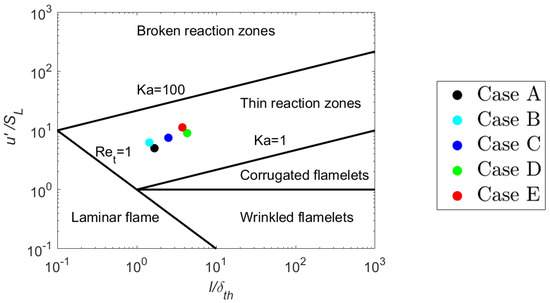
Figure 1. Initial conditions of the statistically planar turbulent premixed methane–air flames on the combustion regime diagram.

Table 2. List of initial simulation parameters and nondimensional numbers.

Case	A	B	C	D	E
$u^{\prime }/S_L$	5.0	6.25	7.5	9.0	11.25
$l/{\delta }_{th}$	1.67	1.44	2.5	4.31	3.75
$Da$	0.33	0.23	0.33	0.48	0.33
$Ka$	8.65	13.0	13.0	13.0	19.5

A reaction progress variable can be defined as

$$c=\frac{Y-Y_0}{Y_{\infty }-Y_0}$$

(2)

where $Y$ is the mass fraction of a chosen species, and subscripts $0$ and $\infty$ indicate the values in the unburned and fully burned gases, respectively. Any major product or reactant with a monotonic behaviour can be chosen for the definition of $c$, and for the purpose of this analysis, methane ($Y_{C{H}_4}$) was selected. Based on the reaction progress variable $c$, an alternative flame thickness similar to the thermal flame thickness can be defined in the following manner:

$${\delta }_L=\frac{c_{max}-c_{min}}{\mathit{max}{\left|\nabla c\right|}_L}$$

(3)

The reaction progress variable can also be defined based on temperature as $c_T=\left(T-T_0\right)/\left(T_{ad}-T_0\right)$, where $T$is the instantaneous dimensional temperature. Due to the possibility of superadiabatic temperatures, the use of $c_T$ can potentially be problematic. Nevertheless, in the case of SC DNS, $c_T$ and $c$ become identical for unity-Lewis-number, adiabatic, low-Mach-number conditions, and under these conditions, we have ${\delta }_{th}={\delta }_L$ and $c_T=c.$ However, for detailed chemistry, this flame thickness can be notably smaller than the thermal flame thickness and depends on the choice of reaction progress variable. For the stoichiometric methane–air flame simulations conducted here, one obtains ${\delta }_L=0.27\mathrm{mm}$ and ${\delta }_{th}=0.43\mathrm{mm}$. An alternative and frequently used definition of flame thickness is the Zel’dovich flame thickness given by

$${\delta }_z=\frac{D_{th,0}}{S_L}$$

(4)

where $D_{th,0}$ is the thermal conductivity in the unburned gas. If one assumes that $\rho D_{th}~{\left(T/T_0\right)}^r$, one can estimate ${\delta }_{th}/{\delta }_Z\approx 2{\left(T_{ad}/T_0\right)}^r$ following the arguments in [2]. For the SC simulations, $\rho D_{th}$ is assumed to be a constant, and hence, $r=0,$ while for the case of DC, one has $r=0.7$ [5]. This shows that ${\delta }_{th}/{\delta }_Z\approx 2$ in the case of SC, while in the case of DC, we have ${\delta }_{th}/{\delta }_Z\approx 2{\left(T_{ad}/T_0\right)}^{0.7}$, which is roughly $8.2$because $T_{ad}/T_0=\left(\mathsf{\tau }+1\right)=7.5$. This discussion demonstrates that under the current assumptions, it is not possible to simultaneously maintain the same thermal and Zel’dovich flame thickness in SC and DC DNS, and a decision had to be taken. Using the same thermal flame thickness allowed using the same computational mesh (using ${\delta }_Z$ would have resulted in considerable under-resolution of the SC case), and for simplicity, this approach was chosen. However, one drawback is that the kinematic viscosity is about a factor of four higher in SC compared to DC using the above scaling arguments together with Equation (4). Repeating the analysis for SC with temperature-dependent material properties is left for future work, but this will not diminish the value of the present results because they are based on the same assumptions that are often made for theoretical analysis of combustion.

3. Results

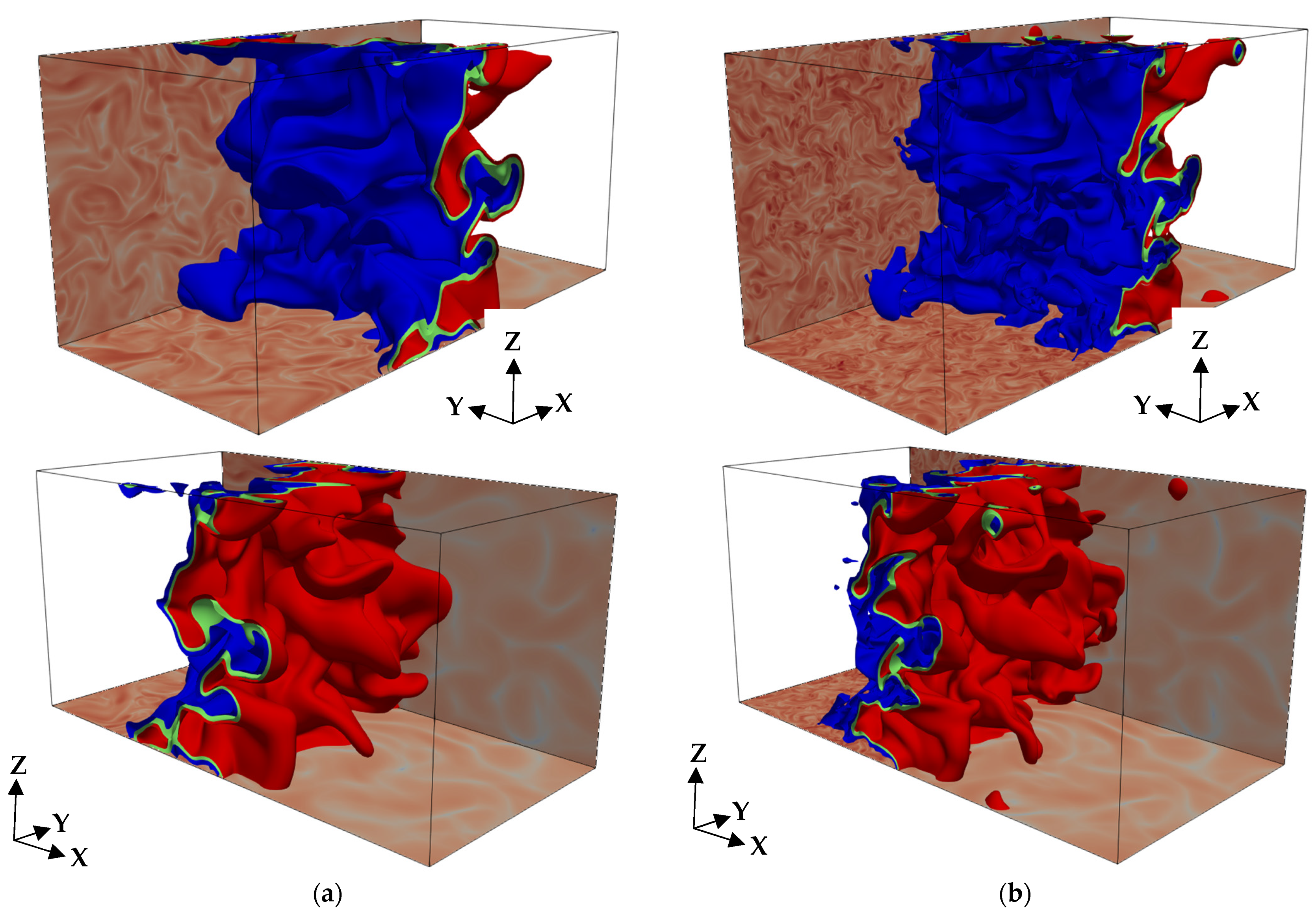
Isosurfaces of reaction progress variable at the time when statistics were extracted, corresponding to one chemical timescale ${\delta }_{th}/S_L$, are shown in Figure 2a–e for Cases AD to ED, respectively. The extent of flame wrinkling in general increases from Cases AD to ED with increasing value of turbulence intensity $u^{\prime }/S_L$. Moreover, the contours of $c$ representing the preheat zone (i.e., $c$ < 0.5) are much more distorted than those representing the reaction zone (i.e., 0.7 < $c$ < 0.9). Furthermore, it can be observed that increasing Karlovitz number increases the scale separation between the flame thickness ${\delta }_{th}$ and the Kolmogorov length $\eta$, such that turbulent eddies can enter the preheat zone and distort the flame structure. Figure 3 exemplarily shows a front and back view of the flame for Cases DS and DD. Turbulence decays across the flame, as clearly visible from the vorticity magnitude, due to a rise in kinematic viscosity with temperature and dilatation rate within the flame. The increased kinematic viscosity leads to a faster dampening of small structures such that the large-scale structures become more dominant, which is clearly visible in Figure 3. This effect is further enhanced by dilatation rate, which acts to stretch turbulent structures. As explained in Section 2, it is not possible to simultaneously match both flame thicknesses ${\delta }_{th}$ and ${\delta }_Z$ for SC and DC simulations, and within the context of this work, the thermal flame thickness was kept constant. This implies a higher viscosity for the SC simulations, and therefore, turbulence decays faster in the SC case compared to the DC case. This effect is reflected in the higher small-scale wrinkling of the DC simulations compared to the SC case, as visible in Figure 3. Nevertheless, it can be clearly seen that the flame structures are characterized by very similar flame topologies.

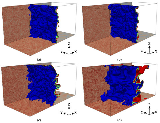
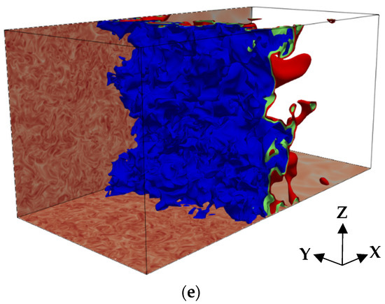
Figure 2. Isosurfaces of reaction progress variable $c$, where blue, green, and red colors represent $c=0.1$, $c=0.5$, $c=0.9$ isolevels, respectively. The vorticity magnitude is shown on the x − y and x − z planes on a logarithmic scale, where red and blue represent high and low vorticity magnitude, respectively. (a–e) Cases AD–ED.

Figure 3. Isosurfaces of reaction progress variable $c$, where blue, green, and red colors represent $c=0.1$, $c=0.5$, $c=0.9$ isolevels, respectively. The statistically planar flame is shown in a front and back view. The vorticity magnitude is shown on the x − y and x − z planes on a logarithmic scale, where red and blue represent high and low vorticity magnitude, respectively. (a) Case DS; (b) Case DD.

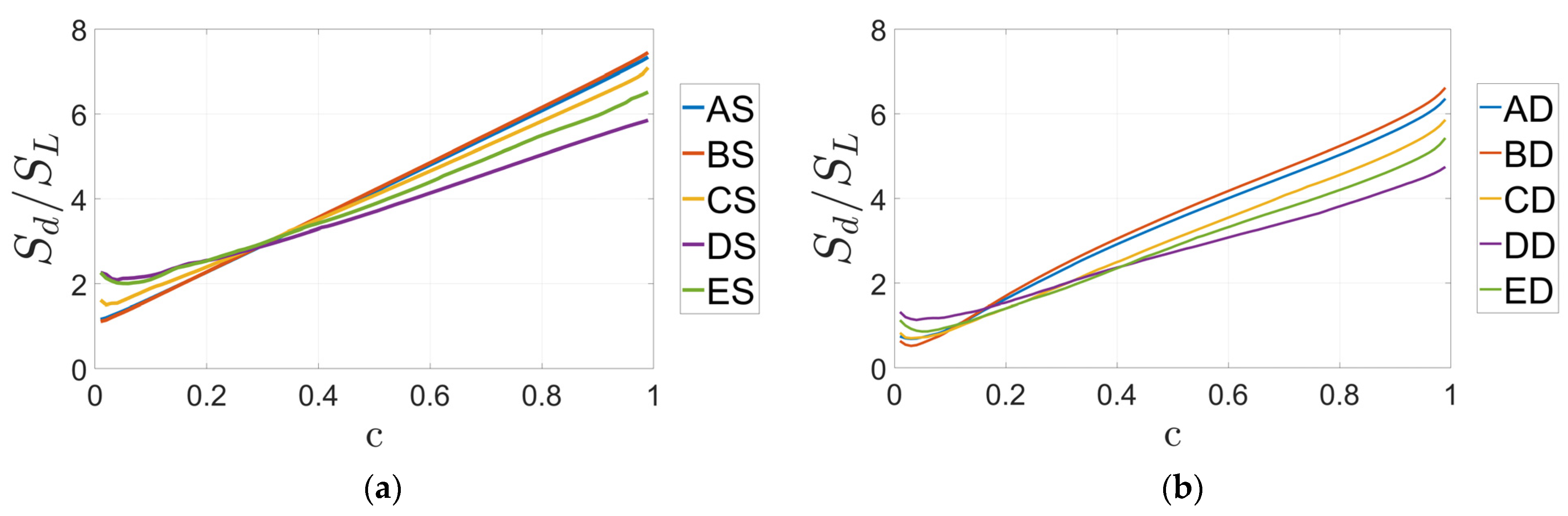
Mean variations of normalized displacement speed $S_d/S_L$ across the flame for Cases A–E for (a) simple chemistry and (b) detailed chemistry are shown in Figure 4. It can be seen from Figure 4 that displacement speed decreases from Case B to A to C to E to D, and this is consistent for SC and DC simulations. The variation in displacement speed for different cases can be explained using asymptotic theory [2,36], which shows that displacement speed $S_d$ decreases with increasing stretch rate $K$ for positive Markstein length (as expected for unity Lewis number flames). The stretch rate $K$ is defined as

$$K=a_T+2{\kappa }_m{S}_d$$

(5a)

$$a_T=\left({\delta }_{ij}-N_i{N}_j\right)\left(\frac{\partial u_i}{\partial x_j}\right)$$

(5b)

$${\kappa }_m=\frac{1}{2}\nabla \cdot \overrightarrow{N}$$

(5c)

where $a_T$ denotes the tangential strain rate, ${\kappa }_m$ is the mean curvature of a $c$isosurfaces, and $\overrightarrow{N}=-\nabla c/\left|\nabla c\right|$ is the flame normal vector pointing into the reactants. Displacement speed can be decomposed into a reactive ($S_r$) normal diffusion ($S_n$), and tangential diffusion component ($S_t$) following [16,17]

$$S_r=\frac{\dot{w}}{\rho \left|\nabla c\right|}$$

(6a)

$$S_n=\frac{\overrightarrow{N}.\nabla \left(\rho D_c\overrightarrow{N}.\nabla c\right)}{\rho \left|\nabla c\right|}$$

(6b)

$$S_t=-2D_c{\kappa }_m.$$

(6c)

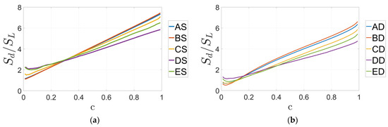
Figure 4. Mean variation of normalized displacement speed $S_d/S_L$ across the flame for Cases A–E for (a) simple chemistry and (b) detailed chemistry simulations.

In the thin reaction zones regime, for $Ka>1$, the tangential diffusion component becomes dominant [39] such that the stretch rate can be approximated by $K\approx a_T-4D_c{\kappa }_m^2$. A simple model for tangential strain rate [50] indicates that $a_T~1/{\tau }_{\eta }$, where the Kolmogorov time scale is given by ${\tau }_{\eta }=\sqrt{\nu /\epsilon }$, with $\epsilon$ being the dissipation rate of turbulent kinetic energy that can be estimated as $\epsilon ~u^{\prime }{}^3/l$. This shows that $a_T$ can, for constant $S_L/{\delta }_{th }$, alternatively be scaled with the Karlovitz number $a_T\sim Ka S_L/{\delta }_{th }$, whereas ${\kappa }_m^2$ can be scaled in terms of the Kolmogorov length scale $\eta$ as ${\kappa }_m^2~1/{\eta }^2$, which also suggests that $D_c{\kappa }_m^2~Ka S_L/{\delta }_{th }$. This argument suggests that the stretch rate increases ($S_d$ decreases) with increasing $Ka$, provided all other parameters are held constant. This is mostly consistent with the behavior shown in Figure 4. The mean value of $S_d$ tends to decrease with increasing $Ka$.

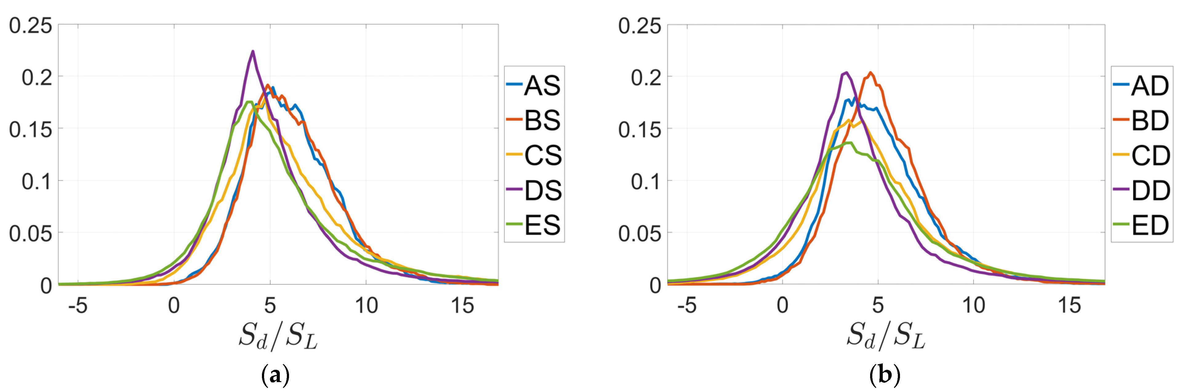
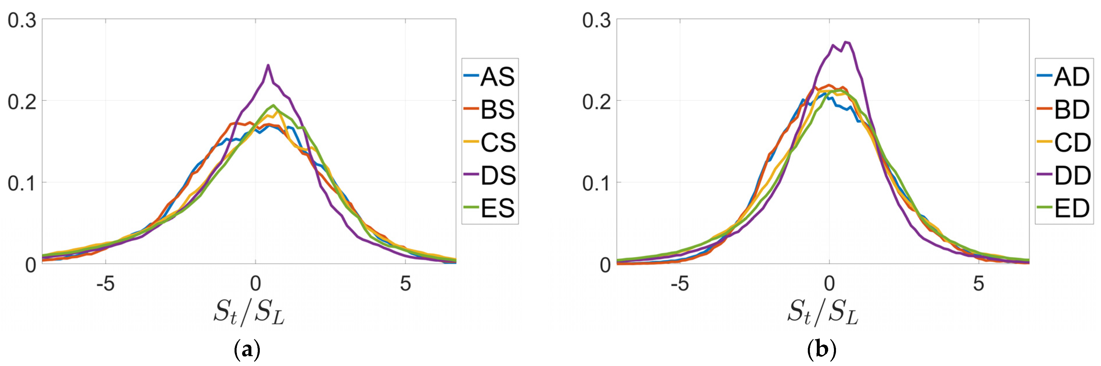
The behavior discussed before is consistent with the Probability Density Functions (PDF) of normalized displacement speed $S_d/S_L$ on the $c$= 0.8 progress-variable isosurface shown for Cases A–E in Figure 5. Following the suggestion of Peters [39] and previous DNS studies [15,16,17,18,19], the PDFs in Figure 5 are presented for a progress variable isosurfaces in the reaction layer, close to the location of maximum reaction rate $c\approx 0.8$, and the same approach is adopted for the remaining discussion. There is good qualitative agreement between both approaches, SC and DC. Further, Figure 5 shows that there is a non-negligible probability of obtaining negative displacement speeds, especially for Cases C, D, and E.

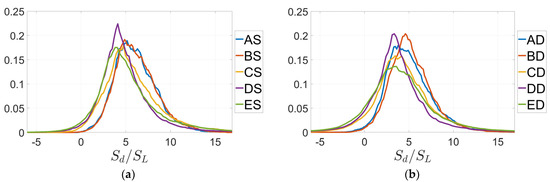
Figure 5. PDF of normalized displacement speed $S_d/S_L$ on c = 0.8 isosurface for Cases A–E for (a) simple chemistry and (b) detailed chemistry simulations.

In order to explain this behavior, displacement speed is split into $S_d=\left(S_r+S_n\right)+S_t$, where the combined contributions of $S_r$ and $S_n$ can be scaled as $\left(S_r+S_n\right)~{\rho }_0{S}_L/\rho$ [39]. The PDFs of $\left(S_r+S_n\right)$ and $S_t$ on the $c$ = 0.8 progress-variable isosurfaces are shown in Figure 6 and Figure 7, respectively. Once more, there is excellent qualitative and, to a large extent, quantitative agreement between SC and DC simulations in terms of $\left(S_r+S_n\right)$ statistics. Comparing Figure 5 and Figure 6, it becomes obvious that the combined reaction and diffusion component $\left(S_r+S_n\right)$ of displacement speed remains mostly positive in contrast to $S_d$. Consistent also between SC and DC, the PDFs can be grouped into Cases $\left\{\mathrm{A},\mathrm{B}\right\}$ with a narrower distribution of $\left(S_r+S_n\right)$ and Cases $\left\{\mathrm{C},\mathrm{D},\mathrm{E}\right\}$ that exhibit more scatter and are more biased towards the negative values.

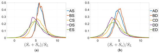
Figure 6. PDF of normalized, combined reaction and normal diffusion components of displacement speed ($S_r+S_n)/S_L$ on $c=0.8$ isosurface for Cases A–E for (a) simple chemistry and (b) detailed chemistry simulations.

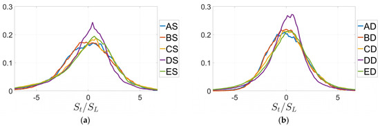
Figure 7. PDF of normalized tangential diffusion components of displacement speed $S_t/S_L$ on $c=0.8$ isosurface for Cases A–E for (a) simple chemistry and (b) detailed chemistry simulations.

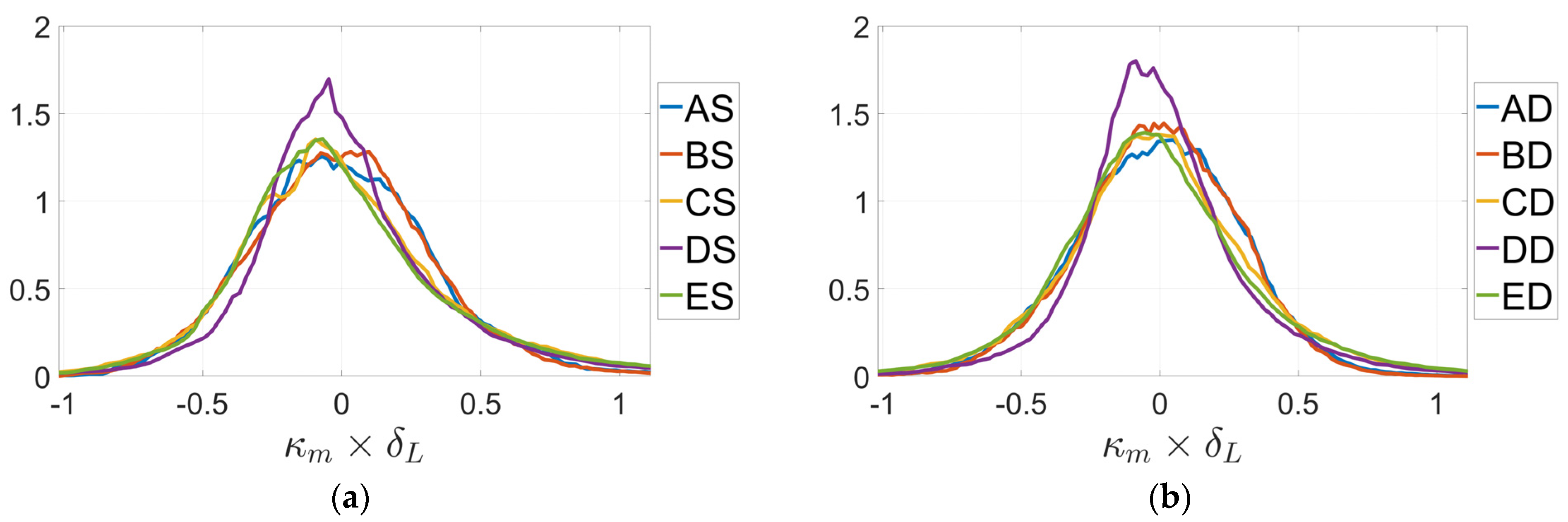
The aforementioned observations show that tangential diffusion component $S_t$ must be mainly responsible for the occurrences of negative $S_d$, and the corresponding PDFs are shown in Figure 7. The PDFs of $S_t$ are characterized by a peak value close to zero and a nearly symmetric distribution with a slightly longer tail towards the negative values for both SC and DC simulations. The $S_t$ PDFs for Cases A and B with a smaller length scale are more concentrated around the mean compared to the larger length scale of Cases C–E, which exhibit longer tails. According to Equation (6), $S_t$ is perfectly negatively correlated with ${\kappa }_m$, and hence, the ${\kappa }_m$ PDFs in Figure 8 behave the same as the $S_t$ PDFs but mirrored at the $y$-axis.

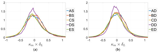
Figure 8. PDF of normalized mean curvature ${\kappa }_m\times {\delta }_L$ on $c=0.8$ isosurface for Cases A–E for (a) simple chemistry and (b) detailed chemistry simulations.

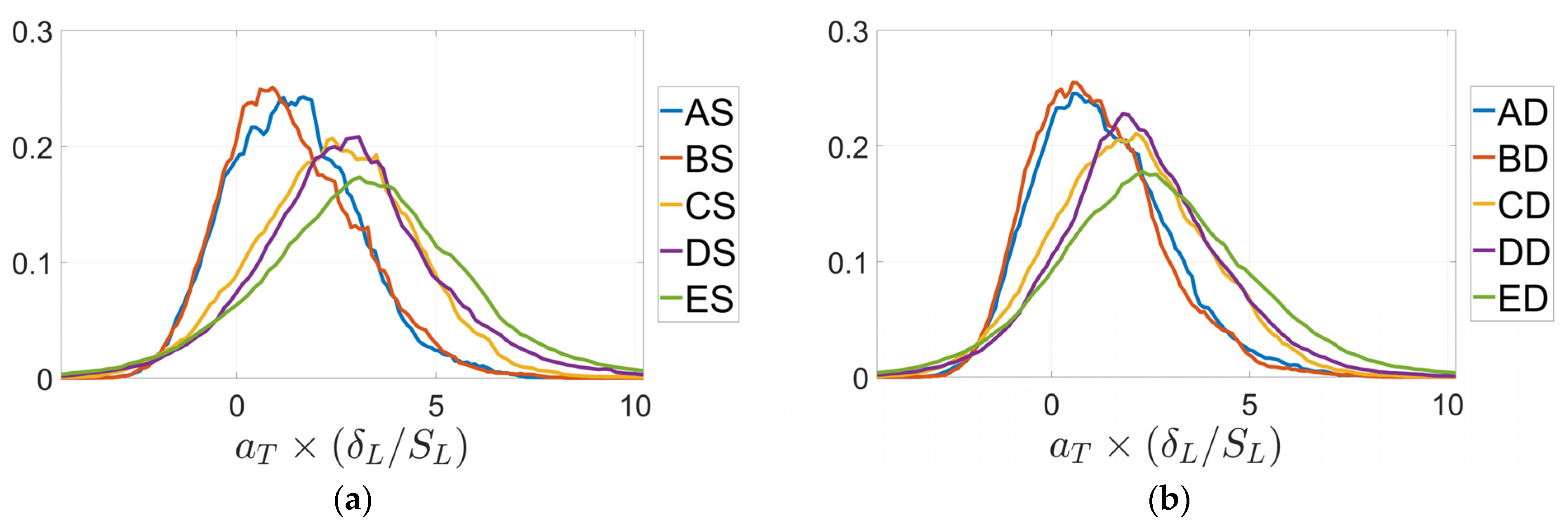
To complete the picture, Figure 9 shows the PDF of normalized tangential strain rate $a_T\times {\delta }_L/S_L$ on the $c=0.8$ progress-variable isosurface for Cases A–E for both SC and DC DNS. It has already been mentioned that $a_T\sim Ka S_L/{\delta }_{th }$, but this equation was derived for a material surface under isotropic turbulence [50], which can be expected to resemble flame propagation for large values of $Ka$, and especially for large values of $R{e}_t$. Figure 9 shows that the width of the tangential strain rate PDF tends to increase with increasing $Ka$ towards positive values. Nevertheless, Cases B, C, and D feature the same Karlovitz number, but Case B behaves differently to Cases C and D. The different behavior of Case B can be explained by the considerably smaller values of $R{e}_t$ and $Ka$, where dilatation effects are still strong in comparison to turbulent straining, and the simple scaling $a_T\sim Ka S_L/{\delta }_{th }$might not be valid.

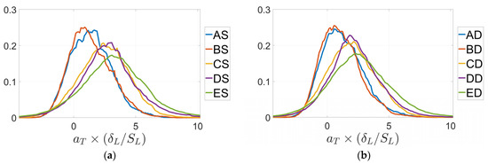
Figure 9. PDF of normalized tangential strain rate $a_T\times {\delta }_L/S_L$ on $c=0.8$ isosurface for Cases A–E for (a) simple chemistry and (b) detailed chemistry simulations.

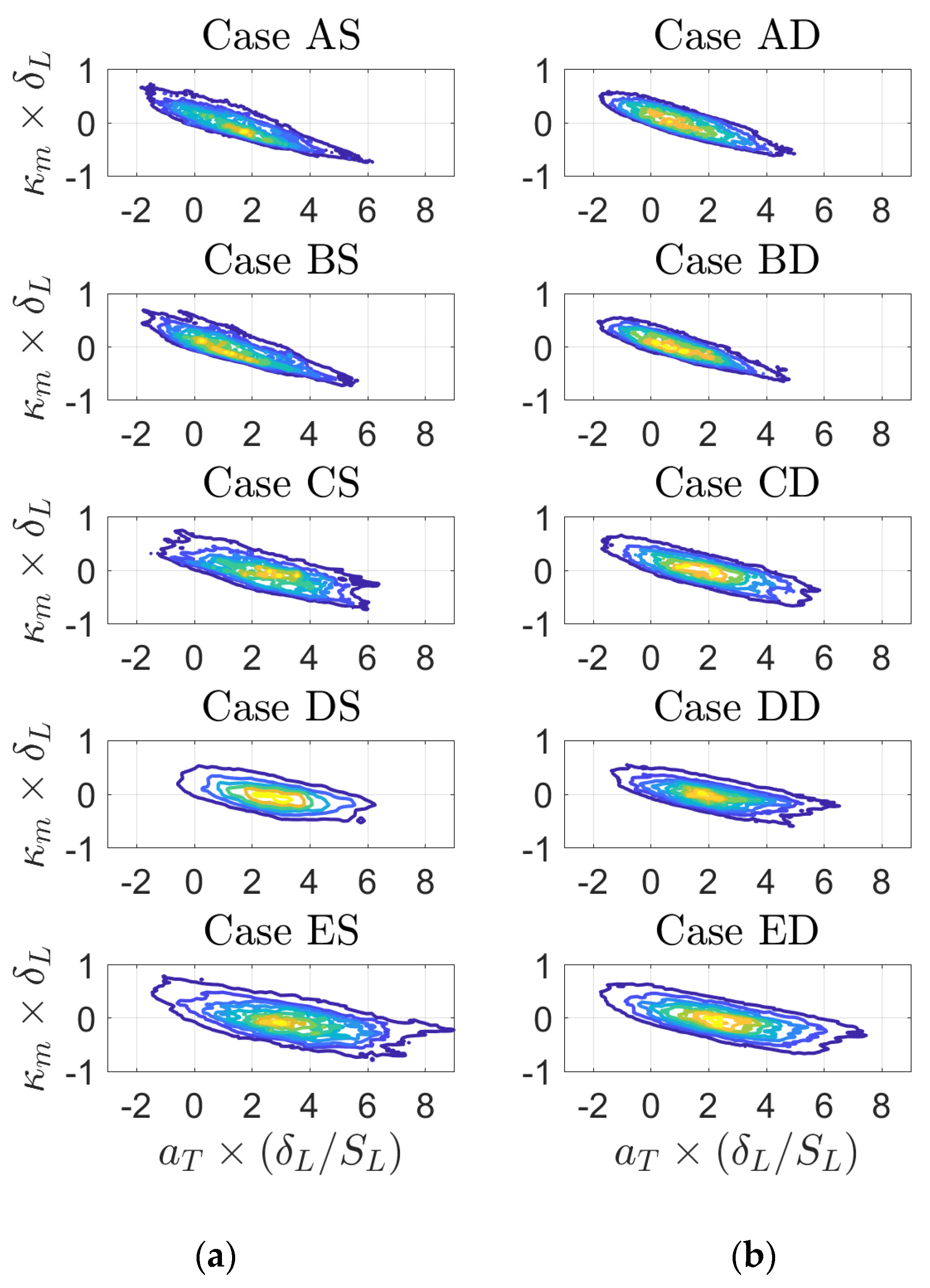
To understand the interrelation between tangential strain rate and curvature, it is worth investigating the joint PDF between $a_T$ and ${\kappa }_m$, which is shown in Figure 10 for all cases for the $c=0.8$ isosurface of reaction progress variable. Consistent with earlier analysis [19,51,52], Figure 10 shows a negative correlation between $a_T$and ${\kappa }_m$. The negative correlation between $a_T$ and ${\kappa }_m$ arises principally due to heat release, and thus the correlation strength weakens with increasing Karlovitz number [51,52], as can be seen in Figure 10. The negative correlation between $a_T$ and ${\kappa }_m$ can be explained in the following manner. In turbulent premixed flames, dilatation rate remains negatively correlated with curvature due to focusing of heat in the negatively curved regions and defocusing of heat in the positively curved regions [52]. The dilatation rate can be expressed in terms of tangential $a_T$ and normal strain rate $a_N$ in the following manner:

$$\nabla \cdot \overrightarrow{u}=a_T+a_N$$

(7)

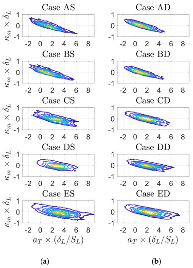
Figure 10. Joint PDF of normalized tangential strain rate $a_T\times {\delta }_L/S_L$ and normalized mean curvature ${\kappa }_m\times {\delta }_L$ on $c=0.8$ isosurface for Cases A–E for (a) simple chemistry and (b) detailed chemistry simulations.

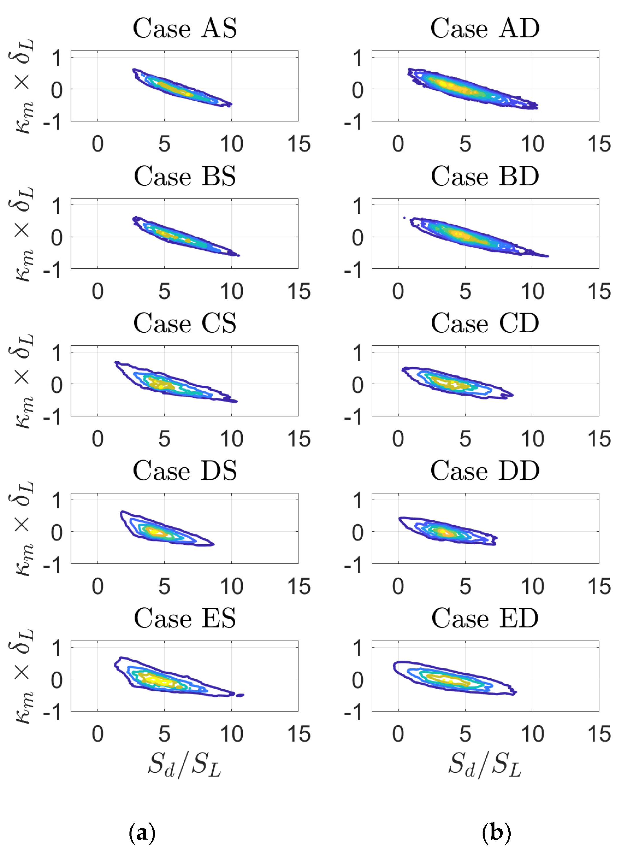
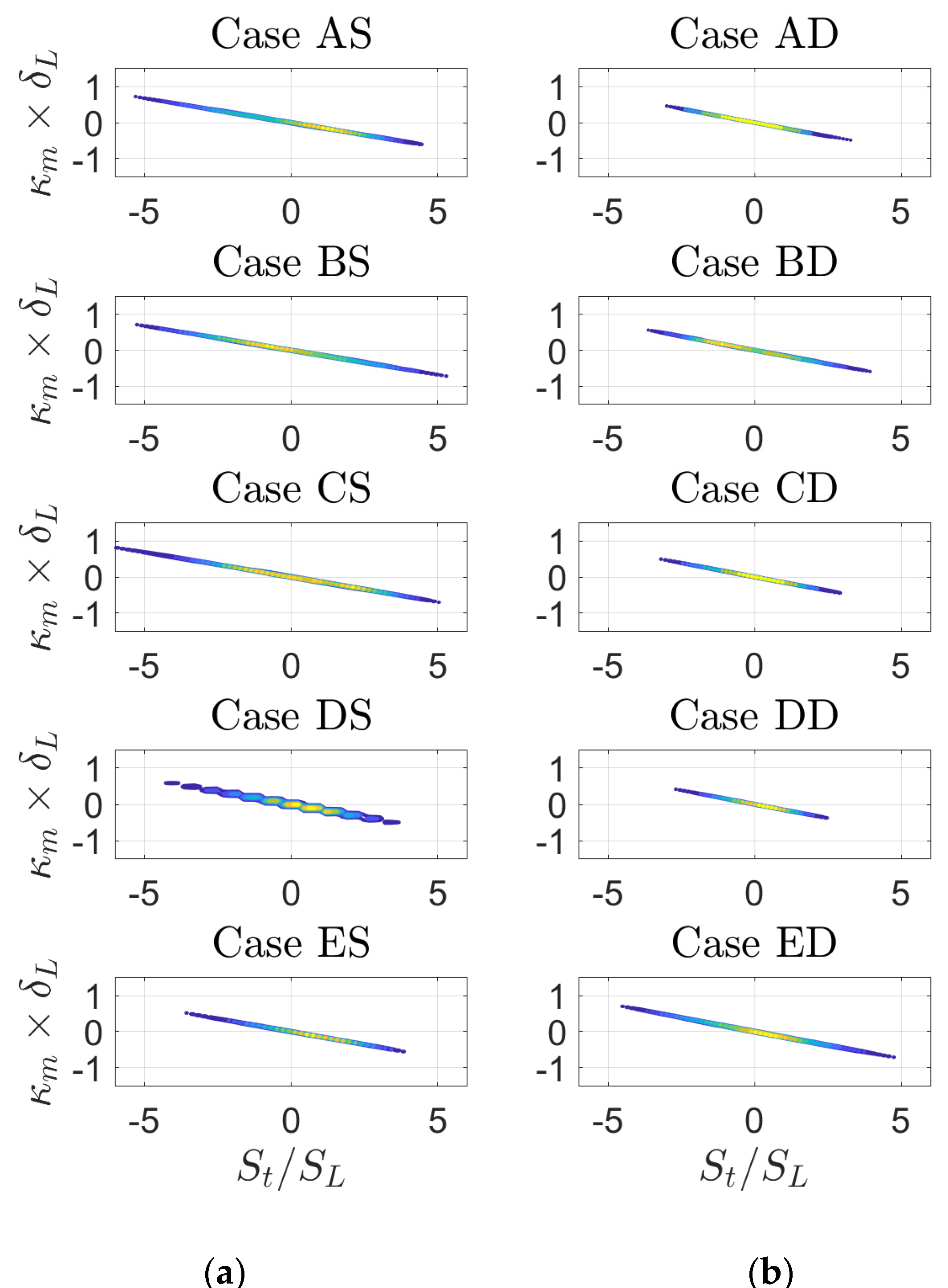
Equation (7) indicates that $\nabla \cdot \overrightarrow{u}$ and $a_T$ are (for $a_N\approx const$) expected to correlate positively, and because of the negative correlation between $\nabla \cdot \overrightarrow{u}$ and ${\kappa }_m$, a negative correlation between $a_T$ and ${\kappa }_m$ is obtained as a result of streamline divergence or convergence in front of curved regions in premixed flames [52]. A negative (positive) correlation between ${\kappa }_m$ and a general quantity $Q$ in general implies a positive (negative) correlation between $a_T$ and $Q$ due to the negative correlation between $a_T$ and ${\kappa }_m$. Hence, for the sake of brevity, the joint PDFs in the following discussion are presented only in terms of curvature correlations. Figure 11 shows that the normalized displacement speed $S_d/S_L$ is nonlinearly, negatively correlated with curvature ${\kappa }_m$, whereas the normalized tangential diffusion component of displacement speed $S_t$ is deterministically negatively correlated with curvature with a correlation coefficient of −1.0, as shown in Figure 12. This demonstrates that the nonlinearity of the $S_d-{\kappa }_m$ correlation originates due to curvature dependance of $\left(S_r+S_n\right)$, and the corresponding joint PDFs are shown in Figure 13. The results obtained from SC and DC simulations show very good qualitative and at least reasonable quantitative agreement, and these observations are consistent with earlier DC and SC simulations [13,14,15,16,17,18,51,52].

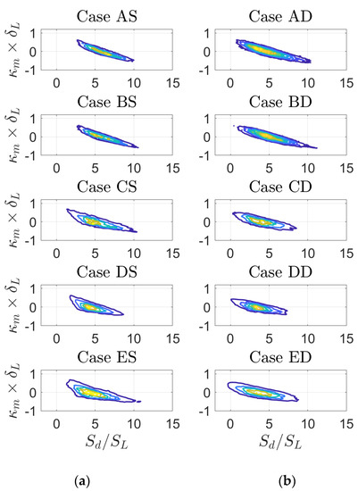
Figure 11. Joint PDF of normalized displacement speed $S_d/S_L$ and normalized mean curvature ${\kappa }_m\times {\delta }_L$ on $c=0.8$ isosurface for Cases A–E for (a) simple chemistry and (b) detailed chemistry simulations.

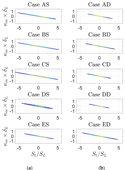
Figure 12. Joint PDF of normalized tangential diffusion components of displacement speed $S_t/S_L$ and normalized mean curvature ${\kappa }_m\times {\delta }_{th}$ on $c=0.8$ isosurface for Cases A–E for (a) simple chemistry and (b) detailed chemistry simulations.

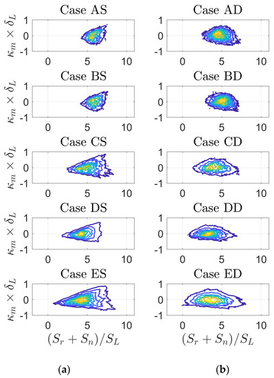
Figure 13. Joint PDF of normalized, combined reaction and normal diffusion components of displacement speed $\left(S_r+S_n\right)/S_L$ and normalized mean curvature ${\kappa }_m\times {\delta }_L$ on $c=0.8$ isosurface for Cases A–E for (a) simple chemistry and (b) detailed chemistry simulations.

In order to explain the weak correlation between $\left(S_r+S_n\right)$ and ${\kappa }_m$, it is important to understand that the $S_r-{\kappa }_m$ and $S_n-{\kappa }_m$ correlations are influenced by the negative correlation between ${\kappa }_m$ and $a_T$ and also by the $a_T$ dependences of $S_r$ and $S_n$. In the case of low Mach number and unity Lewis number flames, the reaction rate $\dot{\omega }$ is independent of curvature, and thus, according to Equation (6) the $S_r-a_T$ correlation is governed by the correlation $\left|\nabla c\right|-a_T$. However, in the case of detailed chemistry, there might be a significant correlation between $\dot{\omega }$ and ${\kappa }_m$, which also depends on the choice of reaction progress variable. A detailed discussion of these effects will be provided in part 2 of this paper and is omitted here for avoiding unnecessary repetition. For the sake of self-consistency, it is briefly mentioned here that Equation (7) suggests that (for constant dilatation rate) $a_T$ and $a_N$ are negatively correlated. Further, a compressive (i.e., negative) normal strain rate causes local thinning, which acts to increase the scalar gradient $\left|\nabla c\right|.$ This suggests that $\left|\nabla c\right|$ is positively correlated with $a_T$ but negatively correlated with $a_N$, and this acts to induce a negative correlation between $S_r$ and $a_T$. This correlation consequently induces a positive correlation between $S_r$ and ${\kappa }_m$. The magnitude of the flame normal diffusion rate $\left|\overrightarrow{N}\cdot \nabla \left(\rho D\overrightarrow{N}\cdot \nabla c\right)\right|$ can be scaled using the flame thickness $\delta$ as $~\rho D/{\delta }^2$ [51], whereas the flame thickness scales as $\delta ~{\left|\nabla c\right|}^{-1}$. Hence, Equation (6) suggests that $S_n$ scales as $-D/\delta$ towards the product side where the normal diffusion component is negative [12,14,52]. This finally yields a negative correlation between $S_n$ and ${\kappa }_m$in the reaction zone. The positive correlation between $S_r$ and ${\kappa }_m$ and the negative correlation between $S_n$ and ${\kappa }_m$ result in a net weak correlation between $\left(S_r+S_n\right)$ and ${\kappa }_m$ as visible in Figure 13.

4. Discussion

The foregoing discussion demonstrated an excellent qualitative and a reasonable quantitative agreement between simulation results from SC and DC DNS. While the focus of this work was the comparison of flame propagation statistics from SC and DC DNS of statistically planar turbulent premixed flames, based on the same computational setup and using the same numerical schemes, an extensive discussion of the physical mechanism responsible for the observed behavior can be found in Refs. [51,52]. In particular, the present database extends the earlier SC work reported in [51] to detailed chemistry simulations, without changing any of the conclusions. All widely used modeling approaches known to the authors were originally developed based on simple chemistry assumptions, such as the level-set [39], Flame Surface Density (FSD)-based [40] modeling methodologies, the artificially thickened flames (ATFs) [53], or the Bray–Moss–Libby (BML) [54] formalism. Despite its admitted limitations, as discussed in Table 2, the present results suggest that SC DNS simulations, without any doubt, should continue to play an important role in future combustion research because of their potential to provide reliable data at a much smaller computational cost and lower carbon footprint or alternatively because of their potential to explore physics at larger Reynolds numbers, higher pressure, or more realistic, larger, computational domains. Questioning the value of SC assumptions, in general, amounts to doubting the aforementioned modeling methodologies, as well as most of the theoretical knowledge that we have about turbulent premixed flames, such as the theories on flame instability or flame stretch rate, as reviewed in [36].

5. Conclusions

Flame propagation statistics from three-dimensional simple chemistry and transport DNS were compared to results obtained from detailed chemistry and transport simulations. To this end, a new DNS database was established encompassing five SC and the corresponding five DC simulations of statistically planar turbulent premixed, stoichiometric methane–air flames for a range of Damköhler, Karlovitz, and turbulent Reynolds numbers. Both methodologies use nearly identical numerical methods and identical initial and boundary conditions. The statistics of displacement speed and its different components, tangential strain rate, and mean curvature were discussed in detail too, along with their interdependencies, and it was found that all conclusions drawn from earlier [51] or the present SC simulations remain valid in the context of DC DNS. In particular, it is observed that the mean displacement speed decreases with increasing Karlovitz number. The variation in flame stretch rate was demonstrated to affect the displacement speed statistics, which were consistently captured from both approaches. The joint PDFs obtained from SC and DC simulations show remarkable qualitative similarities, indicating that local flame propagation statistics can be captured reasonably well using simplified assumptions of chemistry and transport. While the qualitative agreement between SC and DC DNS was found to be excellent, small quantitative differences can indeed be observed. However, it will be shown in the second part of this work that these uncertainties are of the same order of magnitude as the uncertainties arising from the definition of the reaction progress variable in the case of DC simulations.

Advantages and disadvantages of SC and DC DNS were discussed in detail. While SC is certainly not well suited to study the autoignition or formation of pollutants, it offers the possibility for unambiguous data analysis (e.g., no uncertainty in terms of reaction progress variable definition), which makes it convenient to compare the results with analytical derivations. This makes SC DNS a valuable tool for studying turbulence–chemistry interaction with a carbon footprint that can easily be a factor of one hundred lower than that of corresponding DC simulations, which easily reaches the magnitude of CO₂ emissions from transatlantic flights. It has been recently recognized in several disciplines (e.g., astronomy or computer science) that there is an undeniable environmental impact of HPC [9,10]. Hence, it is argued that the methods for scientific analysis should be judiciously chosen in accordance with the requirements of a specific scientific purpose. Translated in the context of this work, this means that SC simulations will often give satisfactory answers to fundamental combustion problems at a much lower cost than DC simulations.

The present work deals with stoichiometric methane–air flames and the investigation of nonunity Lewis number flames is beyond the scope of the present work. Although several analyses indicate that Lewis number effects can at least be qualitatively captured using SC DNS (e.g., [12,26,30]), a quantitative assessment, similar to this work, will be needed in future. It is also well known that flame geometry [15,31] has implications on flame propagation statistics, and quantitative confirmation regarding the accuracy of SC simulations will be needed in this respect as well.

References

- Trisjono, P.; Pitsch, H. Systematic Analysis Strategies for the Development of Combustion Models from DNS: A Review. Flow Turbul. Combust. 2015, 95, 231–259. [Google Scholar] [CrossRef]
- Poinsot, T.; Veynante, D. Theoretical and Numerical Combustion, R.T.; Edwards Inc.: Philadelphia, PA, USA, 2001. [Google Scholar]
- Chen, J.H. Petascale direct numerical simulation of turbulent combustion—Fundamental insights towards predictive models. Proc. Combust. Inst. 2011, 33, 99–123. [Google Scholar] [CrossRef]
- Burali, N.; Lapointe, S.; Bobbitt, B.; Blanquart, G.; Xuan, Y. Assessment of the constant non-unity Lewis number assumption in chemically-reacting flows. Combust. Theory Model. 2016, 20, 632–657. [Google Scholar] [CrossRef]
- Smooke, M.D.; Giovangigli, V. Premixed and Nonpremixed Test Flame Results, in Reduced Kinetic Mechanisms and Asymptotic Approximations for Methane-Air Flames; Springer: Berlin/Heidelberg, Germany, 1991; pp. 29–47. [Google Scholar]
- Hu, E.; Li, X.; Meng, X.; Chen, Y.; Cheng, Y.; Xie, Y.; Huang, Z. Laminar flame speeds and ignition delay times of methane–Air mixtures at elevated temperatures and pressures. Fuel 2015, 158, 1–10. [Google Scholar] [CrossRef]
- Pizzuti, L.; Martins, C.; dos Santos, L.R.; Guerra, D.R. Laminar Burning Velocity of Methane/Air Mixtures and Flame Propagation Speed Close to the Chamber Wall. Energy Procedia 2017, 120, 126–133. [Google Scholar] [CrossRef]
- Bhagatwala, A.; Sankaran, R.; Kokjohn, S.; Chen, J.H. Numerical investigation of spontaneous flame propagation under RCCI conditions. Combust. Flame 2015, 162, 3412–3426. [Google Scholar] [CrossRef] [Green Version]
- Stevens, A.R.H.; Bellstedt, S.; Elahi, P.J.; Murphy, M.T. The imperative to reduce carbon emissions in astronomy. Nat. Astron. 2020, 4, 843–851. [Google Scholar] [CrossRef]
- Zwart, S.P. The ecological impact of high-performance computing in astrophysics. Nat. Astron. 2020, 4, 819–822. [Google Scholar] [CrossRef]
- Icha, P. Entwicklung der Spezifischen Kohlendioxid Emissionen des Deutschen Strommix in den Jahren 1990–2018, Um-Weltbundesamt. Available online: https://www.umweltbundesamt.de/publikationen/entwicklung-der-spezifischen-kohlendioxid-4 (accessed on 2 May 2021).
- Chakraborty, N.; Cant, R.S. Influence of Lewis number on curvature effects in turbulent premixed flame propagation in the thin reaction zones regime. Phys. Fluids 2005, 17, 105105. [Google Scholar] [CrossRef]
- Han, I.; Huh, K.Y. Roles of displacement speed on evolution of flame surface density for different turbulent intensities and Lewis numbers in turbulent premixed combustion. Combust. Flame 2008, 152, 194–205. [Google Scholar] [CrossRef]
- Chakraborty, N. Comparison of displacement speed statistics of turbulent premixed flames in the regimes representing combustion in corrugated flamelets and thin reaction zones. Phys. Fluids 2007, 19, 105109. [Google Scholar] [CrossRef]
- Chakraborty, N.; Klein, M.; Cant, R. Stretch rate effects on displacement speed in turbulent premixed flame kernels in the thin reaction zones regime. Proc. Combust. Inst. 2007, 31, 1385–1392. [Google Scholar] [CrossRef]
- Peters, N.; Terhoeven, P.; Chen, J.H.; Echekki, T. Statistics of flame displacement speeds from computations of 2-D unsteady methane-air flames. Symp. Int. Combust. 1998, 27, 833–839. [Google Scholar] [CrossRef] [Green Version]
- Echekki, T.; Chen, J.H. Analysis of the contribution of curvature to premixed flame propagation. Combust. Flame 1999, 118, 308–311. [Google Scholar] [CrossRef]
- Chen, J.B.; Im, H.G. Stretch effects on the burning velocity of turbulent premixed hydrogen/air flames. Proc. Combust. Inst. 2000, 28, 211–218. [Google Scholar] [CrossRef]
- Chakraborty, N.; Cant, R.S. Effects of strain rate and curvature on surface density function transport in turbulent premixed flames in the thin reaction zones regime. Phys. Fluids 2005, 17, 065108. [Google Scholar] [CrossRef]
- Chakraborty, N.; Hawkes, E.R.; Chen, J.H.; Cant, R.S. Effects of strain rate and curvature on Surface Density Function transport in turbulent premixed CH4-air and H2-air flames: A comparative study. Combust. Flame 2008, 154, 259–280. [Google Scholar] [CrossRef]
- Lipatnikov, A.N.; Nishiki, S.; Hasegawa, T. A direct numerical study of vorticity transformation in weakly turbulent pre-mixed flames. Phys. Fluids 2014, 26, 105104. [Google Scholar] [CrossRef] [Green Version]
- Gao, Y.; Chakraborty, N.; Klein, M. Assessment of sub-grid scalar flux modelling in premixed flames for Large Eddy Simulations: A-priori Direct Numerical Simulation. Eur. J. Mech. Fluids-B 2015, 52, 97–108. [Google Scholar] [CrossRef]
- Papapostolou, V.; Wacks, D.H.; Klein, M.; Chakraborty, N.; Im, H.G. Enstrophy transport conditional on local flow topologies in different regimes of premixed turbulent combustion. Sci. Rep. 2017, 7, 11545. [Google Scholar] [CrossRef] [PubMed] [Green Version]
- Klein, M.; Kasten, C.; Chakraborty, N.; Mukhadiyev, N.; Im, H.G. Turbulent scalar fluxes in Hydrogen-Air premixed flames at low and high Karlovitz numbers. Combust. Theor. Model. 2018, 22, 1033–1048. [Google Scholar] [CrossRef] [Green Version]
- Gao, Y.; Chakraborty, N.; Swaminathan, N. Algebraic Closure of Scalar Dissipation Rate for Large Eddy Simulations of Turbulent Premixed Combustion. Combust. Sci. Technol. 2014, 186, 1309–1337. [Google Scholar] [CrossRef]
- Gao, Y.; Chakraborty, N.; Swaminathan, N. Scalar Dissipation Rate Transport in the Context of Large Eddy Simulations for Turbulent Premixed Flames with Non-Unity Lewis Number. Flow Turbul. Combust. 2014, 93, 461–486. [Google Scholar] [CrossRef]
- Gao, Y.; Minamoto, Y.; Tanahashi, M.; Chakraborty, N. A Priori Assessment of Scalar Dissipation Rate Closure for Large Eddy Simulations of Turbulent Premixed Combustion Using a Detailed Chemistry Direct Numerical Simulation Database. Combust. Sci. Technol. 2016, 188, 1398–1423. [Google Scholar] [CrossRef] [Green Version]
- Nilsson, T.; Langella, I.; Doan, N.A.K.; Swaminathan, N.; Yu, R.; Bai, X.-S. A priori analysis of sub-grid variance of a reactive scalar using DNS data of high Ka flames. Combust. Theory Model. 2019, 23, 885–906. [Google Scholar] [CrossRef] [Green Version]
- Attili, A.; Lamioni, R.; Berger, L.; Kleinheinz, K.; Lapenna, P.E.; Pitsch, H.; Creta, F. The effect of pressure on the hydrodynamic stability limit of premixed flames. Proc. Combust. Inst. 2021, 38, 1973–1981. [Google Scholar] [CrossRef]
- Rasool, R.; Chakraborty, N.; Klein, M. Effect of non-ambient pressure conditions and Lewis number variation on direct numerical simulation of turbulent Bunsen flames at low turbulence intensity. Combust. Flame 2021, 231, 111500. [Google Scholar] [CrossRef]
- Klein, M.; Nachtigal, H.; Hansinger, M.; Pfitzner, M.; Chakraborty, N. Flame Curvature Distribution in High Pressure Turbulent Bunsen Premixed Flames. Flow Turbul. Combust. 2018, 101, 1173–1187. [Google Scholar] [CrossRef] [Green Version]
- Papapostolou, V.; Chakraborty, N.; Klein, M.; Im, H.G. Statistics of Scalar Flux Transport of Major Species in Different Premixed Turbulent Combustion Regimes for H2-air Flames. Flow Turb. Combust. 2019, 102, 931–955. [Google Scholar] [CrossRef] [Green Version]
- Papapostolou, V.; Chakraborty, N.; Klein, M.; Im, H.G. Effects of Reaction Progress Variable Definition on the Flame Surface Density Transport Statistics and Closure for Different Combustion Regimes. Combust. Sci. Technol. 2019, 191, 1276–1293. [Google Scholar] [CrossRef] [Green Version]
- Attili, A.; Luca, S.; Denker, D.; Bisetti, F.; Pitsch, H. Turbulent flame speed and reaction layer thickening in premixed jet flames at constant Karlovitz and increasing Reynolds numbers. Proc. Combust. Inst. 2021, 38, 2939–2947. [Google Scholar] [CrossRef]
- Bouvet, N.; Halter, F.; Chauveau, C.; Yoon, Y. On the effective Lewis number formulations for lean hydrogen/hydrocarbon/air mixtures. Int. J. Hydrog. Energy 2013, 38, 5949–5960. [Google Scholar] [CrossRef]
- Lipatnikov, A.; Chomiak, J. Molecular transport effects on turbulent flame propagation and structure. Prog. Energy Combust. Sci. 2005, 31, 1–73. [Google Scholar] [CrossRef]
- Chakraborty, N.; Herbert, A.; Ahmed, U.; Im, H.G.; Klein, M. Assessment of extrapolation relations of displacement speed for detailed chemistry Direct Numerical Simulation database of statistically planar turbulent premixed flames. Flow Turb. Combust. 2021. [Google Scholar] [CrossRef]
- Echekki, T.; Chen, J.H. Unsteady strain rate and curvature effects in turbulent premixed methane-air flames. Combust. Flame 1996, 106, 184–202. [Google Scholar] [CrossRef]
- Peters, N. Turbulent Combustion; Cambridge University Press: Cambridge, UK, 2000. [Google Scholar]
- Pope, S. The evolution of surfaces in turbulence. Int. J. Eng. Sci. 1988, 26, 445–469. [Google Scholar] [CrossRef]
- Jenkins, K.W.; Cant, R.S. Direct Numerical Simulation of Turbulent Flame Kernels. In Recent Advances in DNS and LES. Fluid Mechanics and Its Applications; Knight, D., Sakell, L., Eds.; Springer: Berlin/Heidelberg, Germany, 1999; Volume 54. [Google Scholar] [CrossRef]
- Wray, A.A. Minimal Storage Time Advancement Schemes for Spectral Methods; Tech. Rep. NASA Ames Research Center: Silicon Valley, CA, USA, 1990. [Google Scholar]
- Poisont, T.; Lele, S.K. Boundary conditions for direct simulation of compressible viscous flows. J. Comp. Phys. 1992, 101, 104–129. [Google Scholar]
- Cant, R.S. SENGA2 Manual, CUED-THERMO-2012/04, 2nd ed.; University of Cambridge: Cambridge, UK, 2013. [Google Scholar]
- Im, H.G.; Chen, J.H. Preferential diffusion effects on the burning rate of interacting turbulent premixed hydrogen-air flames. Combust. Flame 2002, 131, 246–258. [Google Scholar] [CrossRef]
- Kee, R.J.; Rupley, F.M.; Miller, J.A.; Coltrin, M.E.; Grcar, J.F.; Meeks, E.; Moffat, H.K.; Lutz, A.E.; Dixon-Lewis, G.; Smooke, M.D.; et al. CHEMKIN, Collection, Release 3.6; Reaction Design, Inc.: San Diego, CA, USA, 2000. [Google Scholar]
- Kennedy, C.A.; Carpenter, M.H.; Lewis, R. Low-storage, explicit Runge–Kutta schemes for the compressible Navier–Stokes equations. Appl. Numer. Math. 2000, 35, 177–219. [Google Scholar] [CrossRef] [Green Version]
- Klein, M.; Chakraborty, N.; Ketterl, S. A Comparison of Strategies for Direct Numerical Simulation of Turbulence Chemistry Interaction in Generic Planar Turbulent Premixed Flames. Flow Turbul. Combust. 2017, 99, 955–971. [Google Scholar] [CrossRef]
- Rogallo, R.S. Numerical Experiments in Homogenous Turbulence, NASA Technical Memorandum 91416; NASA Ames Research Center: Silicon Valley, CA, USA, 1981. [Google Scholar]
- Cant, R.; Pope, S.; Bray, K. Modelling of flamelet surface-to-volume ratio in turbulent premixed combustion. Symp. Int. Combust. 1991, 23, 809–815. [Google Scholar] [CrossRef]
- Chakraborty, N.; Klein, M.; Cant, R.S. Effects of Turbulent Reynolds Number on the Displacement Speed Statistics in the Thin Reaction Zones Regime of Turbulent Premixed Combustion. J. Combust. 2011, 2011, 1–19. [Google Scholar] [CrossRef] [Green Version]
- Jenkins, K.; Klein, M.; Chakraborty, N.; Cant, R. Effects of strain rate and curvature on the propagation of a spherical flame kernel in the thin-reaction-zones regime. Combust. Flame 2006, 145, 415–434. [Google Scholar] [CrossRef]
- Butler, T.; O’Rourke, P. A numerical method for two dimensional unsteady reacting flows. Symp. Int. Combust. 1977, 16, 1503–1515. [Google Scholar] [CrossRef] [Green Version]
- Bray, K.; Libby, P.A.; Moss, J. Unified modeling approach for premixed turbulent combustion—Part I: General formulation. Combust. Flame 1985, 61, 87–102. [Google Scholar] [CrossRef]
Publisher’s Note: MDPI stays neutral with regard to jurisdictional claims in published maps and institutional affiliations. |
© 2021 by the authors. Licensee MDPI, Basel, Switzerland. This article is an open access article distributed under the terms and conditions of the Creative Commons Attribution (CC BY) license (https://creativecommons.org/licenses/by/4.0/).