Optimization of Phasor Measurement Unit Placement Using Several Proposed Case Factors for Power Network Monitoring

Abstract

Recent developments in electrical power systems are concerned not only with static power flow control but also with their control during dynamic processes. Smart Grids came into being when it was noticed that the traditional electrical power system structure was lacking in reliability, power flow control, and consistency in the monitoring of phasor quantities. The Phasor Measurement Unit (PMU) is one of the main critical factors for Smart Grid (SG) operation. It has the ability to provide real-time synchronized measurement of phasor quantities with the help of a Global Positioning System (GPS). However, when considering the installation costs of a PMU device, it is far too expensive to equip on every busbar in all grid stations. Therefore, this paper proposes a new approach for the Optimum Placement of the PMU problem (OPP problem) to minimize the installed number of PMUs and maximize the measurement redundancy of the network. Exclusion of the unwanted nodes technique is used in the proposed approach, in which only the most desirable buses consisting of generator bus and load bus are selected, without considering Pure Transit Nodes (PTNs) in the optimum PMU placement sets. The focal point of the proposed work considers, most importantly, the case factor of the exclusion technique of PTNs from the optimum PMU locations, as prior approaches concerning almost every algorithm have taken PTNs as their optimal PMU placement sets. Furthermore, other case factors of the proposed approach, namely, PMU channel limits, radial bus, and single PMU outage, are also considered for the OPP problem. The proposed work is tested on standard Institute of Electrical and Electronics Engineering (IEEE)-case studies from MATPOWER on the MATLAB software. To show the success of the proposed work, the outputs are compared with the existing techniques.

1. Introduction

Traditional power system State Estimation (SE) uses information from measurement devices to measure the voltage phasor, bus angle, real and reactive power, power flows, and power injection. Until now, Supervisory Control and Data Acquisition (SCADA) was the only technique for obtaining this information and gathering all the data in real-time with the help of a Remote Terminal Unit (RTU). Advancements in the newly metered technology Phasor Measurement Unit in the late 1980s brought a real change in monitoring, controlling, and protecting the power system. The necessity of Phasor Measurement Units (PMUs) was suggested after the huge blackout that happened in 2003, where almost 55 million people in the USA and Canada were badly affected due to the shortage of power supply [1]. This blackout is considered one of the largest blackouts in the world, after which the use of PMUs was highly recommended. A PMU is a metering device that has the ability to directly measure the voltage phasor of the installed bus and the current phasors of all the lines connected to that PMU installed bus. A large number of PMUs are now being installed in developed countries to monitor, protect, and control the electrical system as a whole [2].

The operation of PMUs is one of the key elements for Smart Grid (SG) implementation. The characteristics of protecting, monitoring, and controlling power systems via SGs are considered to be important factors for future power systems. In the literature [3], a different concept of SG is presented in which virtual power, drivers, and roadmaps are presented for the development of SG throughout the world. A bus is said to be observable from an electrical point of view if all of its electrical quantities (voltages and currents) can be measured, which can easily be done by PMUs. Moreover, PMUs deliver the synchronized information from all the measurements with the support of a Global Positioning System. The phasor information is directly synchronized and transmitted via GPS to the Phasor Data Concentrator (PDC), which is known as the synchro-phasor. The robustness of GPS, accurate results, sampled large chunks of data, relaying processes, and provision of a negligible amount of error have led to the expansion of PMUs. Thus, the measurement obtained from PMUs can easily be calculated in real-time using synchronization and time stamping. This information is imperative to power engineers and operators when the power system faces disturbances or dynamic behavior, which can cause a catastrophic failure [4].

Due to the high economic and infrastructure cost, the PMUs need to be placed optimally in a grid station to obtain the maximum depth of measurement redundancy, and the process of optimally placing PMUs to observe maximum buses is known as the optimal PMU placement problem (OPP problem). Recent research on the OPP problem have found that tactically placing a PMU with the use of Kirchhoff Current Law (KCL) and Ohm’s law would help in determining the behavior of all the buses in a single network. The use of formulation and the robust features of PMUs will lead to reducing the required number of PMUs compared to the number of busses. Different optimization techniques have been used to examine the optimal placement of PMUs, namely Genetic Algorithm (GA), Particle Swarm Optimization (PSO), Tabu Search (TS), greedy algorithm, Integer Linear Programming (ILP), integer quadratic programming, Simulated Annealing (SA), hybrid algorithm (BPSO), Exhaustive Search (ES), Depth-First Search (DeFS), and Minimum Spanning Tree (MST). These algorithms are classified into different techniques; some of them are categorized under the old conventional methods, such as mathematical programming, while most of the recognized techniques, such as PSO and GA, are considered modern heuristic and meta-heuristic methods. However, existing research has shown that most leading conventional techniques, from mathematical programming to heuristic algorithms, that are used for the OPP problem do not provide the optimum placement of PMUs. Thus, a new proposed methodology is implemented, based on meta-heuristics algorithms, to overcome past issues and improve the outcomes of optimum PMUs placement. Most of the prior studies considered different factors to solve the OPP problem, such as conventional measurement, with and without considering zero injection buses (ZIBs), single PMU loss, and channel limits. There are two types of conditional monitoring rules, which are available for the measurement of PMU placement: numerical and topological observability conditions. In the numerical monitoring rule, a large number of mathematical calculations and matrix estimations are involved to solve the OPP problem [3]. In reference [4], an OPP problem is solved using the numerical approach, in which the PMU placement is done by the elimination of critical measurement. These measurements were latter referred to as bad data for the system. In the literature [5], an integer linear programming technique was implemented with the help of a binary adjacent matrix to solve the OPP problem. An integer quadratic program approach is presented in [6], to minimize the number of PMUs and maximize the measurement redundancy. With the help of matrices calculation, the OPP problem was solved using different objectives, including transmission line outage, a normal operating condition in which all the case factors are ignored. A visual representation of observability rules and formulation for the OPP problem has been presented in reference [7], in which the three observability rules are explained in detail to find the parameters of the busbars using the installation of PMUs. In [8], two techniques are used, which aim to decrease the computational burden from the system by removing the virtual information. These techniques solve the OPP problem with the help of the reduction of additional information.

However, the topological observability initially has a graph-type shape to make the complete network into a graphical form. This graph theory searching procedure further arranges the nodes’ characteristics, network types, and connections, which helps in understanding better placement regarding the OPP problem [9]. In [10], the depth-first search method is applied to optimize the minimum number of PMUs using the Power System Analysis Toolbox (PSAT). During this operation, the method assigns the values of binary digits, where digit 1 represents the placement of PMUs in a designated location, while digit 0 represents not taking any interest in the placement of PMUs. An optimization technique, namely differential evaluation, is adopted in [11] for the OPP problem. It finds the best solutions with the enhancement of the particle momentum. A genetic algorithm is used in [12] to find the best placement for PMUs in order to improve the state estimation performance by finding the irrelevant information from the system. In the literature [13], a simulated annealing technique is presented considering the cost factors of a PMU device. The optimal placement of PMUs is achieved by exposing the dynamic information in the system. This dynamic information not only assists in finding the complex power measurement but is also useful in providing the placement of PMUs. In reference [14], Particle Swarm Optimization (PSO) is used to solve the OPP problem. In the same literature, it is stated that different locations have different impacts on the placement of PMUs.

In this approach [15], the problem was solved by considering topological-based node equations and the removal of some of the nodes from the optimum locations, which only have one incident branch. However, in this paper, the proposed approach uses the formulation of a topological-based meta-heuristic approach to deal with the optimal solutions, considering numerous factors such as normal operating conditions, the removal of unwanted nodes from the placement sets, single PMUs failure, and PMU channel limits. Moreover, it is stated that a PMU has a limited number of channels that can only observe a limited number of buses, and these depend on the manufacturing of the device. In other words, if it has a fewer number of channels, its measurement ability is more restricted than a PMU device which has a greater number of channels, even though the channel limit factor is the least important issue. Prior literature has not taken PTNs into account in their simulation results as there is no benefit in selecting them as an optimum PMU location because there is no power injection nor power flowing through them and they cannot give observability coverage to other buses in a network. Thus, the focal point of this proposed work is to remove the PTNs from the optimum PMU placement sets. Hence, this presented work examines the application of the proposed work to solve the problem of PMU placement through considering the normal operating conditions, removal of unwanted nodes, single PMUs loss, and PMU channel limit.

2. Materials and Methods

The initial material for the OPP problem is derived from the basic equations, which are used to construct the concept of an adjacent matrix for further connectivity of the network. This matrix consists of binary numbers. This helps in the arrangement of nodes and determination of the connectivity of every node with their incident branches, and assists in finding the optimum locations for PMU placement. The explanation of the binary connectivity adjacent matrix is described in terms of the IEEE-9 bus network (Figure 1), given as Equation (1).

The binary connectivity matrix B is generated with the help of the IEEE-9 bus network

$$B=\left[\begin{array}{ccccccccc}1& 0& 0& 1& 1& 0& 0& 0& 0\\ 0& 1& 0& 0& 0& 0& 0& 1& 0\\ 0& 0& 1& 0& 0& 0& 1& 0& 0\\ 1& 0& 0& 1& 0& 0& 0& 0& 1\\ 1& 0& 0& 0& 1& 1& 0& 0& 0\\ 0& 0& 1& 0& 1& 1& 1& 1& 0\\ 0& 0& 0& 0& 0& 1& 1& 1& 0\\ 0& 1& 0& 0& 0& 0& 1& 1& 1\\ 0& 0& 0& 1& 0& 0& 0& 1& 1\end{array}\right]$$

(1)

2.1. Parameter Selection

Parameter selection is very crucial when proposing a new optimization method, and the choice of these parameters defines the performance of the algorithm. Careful selection of the parameters ensures that the implementation of an algorithm provides a meaningful outcome for the purposes of validation with previous studies. The selection of the defined proposed parameters is listed below in the same section.

2.1.1. Construction of Adjacent Matrix (B)

In the proposed methodology, the consideration of an adjacent matrix B is the first step in initializing its program for the OPP problem. The proposed approach has defined the matrix in two ways; one is mathematical modeling derived from the IEEE-datasets and the other is programming in the MATLAB (Mathworks, Natick, Massachusetts, USA). These describe the function and connection between the elements of matrix B. In the mathematical method, there are always two opposite objectives involved concerning the OPP problem. It describes the installation of the minimum number of PMUs by providing maximum measurement redundancy of the network. Moreover, the proposed methodology structures the equation of matrix B by the standard formula given in Section 2. The modeling of matrix B consists of binary numbering obtained from the standard IEEE-Single Line Diagram (SLD). The IEEE standard SLDs have been helpful for the proposed adjacent matrix B modeling; through this, it becomes easier to make a connectivity matrix between the nodes and the derivation of the constraint function from the connectivity matrix. This approach is taken as the first step to understanding and operating the process of the OPP problem. Moreover, the proposed methodology binary matrix B has two digits involved in taking a decision, i.e., (0/1). These digits make decisions using binary numbers; digit 1 indicates the optimum location for the PMU installation, whereas digit 0 indicates that there is no interest in certain locations.

The proposed work uses programming language by implementing the coding in the MATLAB programming software. The proposed approach adopts a certain number of parameters to begin the OPP problem case in the MATLAB optimization-based software using a matrix B. To make the connection to an adjacent matrix, the proposed method conducted a study on the IEEE-datasets in which the parameters of the IEEE-branch data were carried out. The branch data comprises the connection between two buses and the characteristics of the buses. In the branch data of the IEEE bus network, the line between the two buses is referred to as the branch line or incident line. The starting connection of the line between the buses is named the from-bus (f-bus), and the ending line to the bus is called the to-bus (t-bus). Furthermore, other data are also included in the branch section, such as resistance, reactance, total branch line charging susceptance, transformer rating (MVA), and phase shift angle. The proposed technique locates the f-bus and t-bus in the branch data, and these are mainly useful in constructing the structure of adjacent matrix B regarding the OPP problem in which the linkage between the buses is known by the current incident branch lines, which start at the f-bus and end at the t-bus. The example of a proposed matrix B in the OPP problem concept is intended to be a power system observability, as given below in Equation (2).

$$\begin{array}{c}B=\left[1 0 0 0 0 0 0 1\right]; \left[0 1 0 0 0 0 0 1\right]; \left[0 0 1 0 0 0 0 1\right]; \left[0 0 0 1 0 0 0 1\right];\\ \left[0 0 0 0 1 0 0 1\right]; \left[0 0 0 0 0 1 0 1\right]; \left[0 0 0 0 0 0 1 1\left]; \right[1 1 1 1 1 1 1 1\right]\end{array}$$

(2)

When applying the formulation of the above equation in the algorithm form, then it will become:

$$B=\left[\begin{array}{c}1 0 0 0 0 0 0 1\\ 0 1 0 0 0 0 0 1\\ 0 0 1 0 0 0 0 1\\ 0 0 0 1 0 0 0 1\\ 0 0 0 0 1 0 0 1\\ 0 0 0 0 0 1 0 1\\ 0 0 0 0 0 0 1 1\\ 1 1 1 1 1 1 1 1\end{array}\right]$$

(3)

The above Equation (3) explains the initial stage of an 8 $\times$ 8 matrix B, which consists of eight arrays. Each element in the row vector denotes the number of busbars connected to each other in the network, so it contains eight buses with the connectivity of binary digits. In matrix B, the seven arrays ensure that only two incident branches relate to each even bus. However, the eighth row denotes the bus-8 connection in a network with seven connected branches, which means that the PMU should be installed on bus-8. The power system whose given adjacent matrix B will be completely observable if the PMU is installed at bus-8 is represented by the eighth row and the same column.

2.1.2. Sparse Matrix (S)

Another important parameter is considered in the proposed methodology to expedite the construction process of the adjacent matrix B, and this function is called the sparse matrix. It is adopted in the proposed work to manipulate the large dataset available of the IEEE-case studies and is especially used for large data and cannot be implemented in small-level mathematical operations. Its output adjacency matrix is the compressed form of its input version; an example is given in Equations (4) and (5) to show the performance of the sparse function. Its main objective is to enhance the computational performance with the elimination of zero elements from the available datasets, which further improves the efficiency of the algorithm. In the proposed methodology, the sparse function has been useful in efficiently storing the IEEE-dataset with a high ratio of zero components. The selection of the high ratio of zero element information in the proposed operation is helpful in the determination of zero and nonzero elements from the datasets. Other matrices store every element in their memory, regardless of any determination of data, whereas the sparse function only collects nonzero elements. The connection between every incident branch line and the size of the branch data is clearly described in this matrix. It can assign to any two-dimensional MATLAB matrix, and it has the advantage of storing only the nonzero elements in the MATLAB matrix [16]. The sparse function represents in column order; the formatting of the output matrix is shown in column form after the operation on the binary adjacent matrix B and is shown in the below-given equations. There are different types of sparse functions available for optimization purposes, but the proposed approach considers the compressed sparse function operation in the OPP problem as it compresses the large column data into a shorter format for fast analysis. In this OPP problem case, the proposed approach requires outcomes without zero elements, which is why the sparse function has been used in its algorithm. The example of a sparse matrix is illustrated in Equations (4) and (5). The example equations are to demonstrate the performance of a sparse matrix.

Let us suppose the construction of a matrix $\mathrm{n}\times \mathrm{m}$, 8 $\times$ 8, given below:

$$B=\left[\begin{array}{c}\begin{array}{c}0 0 0 0 0 0 0 5\\ 0 6 0 0 0 0 0 0\\ 1 4 0 0 0 0 0 0\\ 0 0 9 0 0 0 0 0\end{array}\\ 0 0 0 0 7 0 0 0\\ 0 0 0 0 0 0 8 0 \\ 0 6 0 0 0 0 0 0\\ 0 0 0 0 0 0 7 0\end{array}\right]$$

(4)

The large matrix is converted into vector order using the sparse function:

$$Sparse \left(S\right)=\begin{array}{c}\left(3,1\right)·1\\ \left(2,2\right)·6\\ \left(7,2\right)·6\\ \left(3,2\right)·4\\ \left(4,3\right)·9\\ \left(5,5\right)·7\\ \left(6,7\right)·8\\ \left(8,7\right)·7\end{array}$$

(5)

The right side of Equation (5) shows the locations of the preferable elements in a matrix, whereas the left side shows the location of the elements in a row and column format. The nonzero elements that come first, according to the row-column order, must be considered on the selection side. This is why it is helpful in the proposed methodology to eliminate the unnecessary elements from the matrix, only showing the result of the nonzero components after converting the matrix into vector form for a fast computational process.

2.1.3. Cuthill–Mackee Permutation

The proposed methodology considers another important parameter in its operation to remove the Pure Transit Nodes, which is called the Cuthill–Mackee Permutation (CMP). It is the last defined parameter of the proposed method and is used to remove the unnecessary nodes of the OPP problem. The proposed methodology adopted this function because it is one of the first heuristics algorithms designed to reduce the reduction of the bandwidth. It moves across the graph, then begins its operation by selecting the random nodes and exploring them with the higher number of branches of the neighboring nodes. The function of the Cuthill–Mackee algorithm is specially implemented in the proposed methodology for sparse matrix nonzero structures. This function is used to permute the sparse matrix; thus, the operation of permutation is considered in the proposed operation for the removal of PTNs from the optimum PMU placement sets in order to arrange the elements of the matrix into a sequence and linear order. It has been instrumental throughout the proposed methodology operation in arranging the network buses/nodes during the process of constructing an adjacent matrix. Moreover, in the proposed approach, this function compresses the large dataset bandwidth and then converts it into a smaller one by properly arranging the nodes in the graph. These nodes are shown as busbars, while the graphs indicate the power network connectivity. For a suitable renumbering of the nodes, the Cuthill–Mackee permutation is named the Reverse Cuthill-Mackee permutation (RCM). To considerate the function of RCM in the proposed approach, the RCM process is applied to the symmetric sparse matrix given below:

Let us consider the $\mathrm{n}\times \mathrm{n}$ with 8 rows and 8 columns $\left(8\times 8\right)$ matrix shown in Equation (6):

$$\mathrm{Input} \mathrm{matrix}=\left[\begin{array}{c}1 0 0 0 0 0 1 0\\ 0 1 0 1 0 0 0 0\\ 1 0 1 0 0 1 1 0\\ 0 1 0 1 0 1 0 0\\ 0 0 0 0 1 0 0 1\\ 0 0 1 1 0 1 0 0\\ 1 0 1 0 0 0 1 0\\ 0 0 0 0 1 0 0 1\end{array}\right]$$

(6)

The above input matrix given in Equation (6) explains the connectivity inside the network, and the responsibility of the RCM function is to transform this connectivity matrix into a graphical shape, which is illustrated in Figure 2:

The resultant output matrix from the RCM algorithm on an $\left(8\times 8\right)$ input matrix is shown in Equation (7):

$$\mathrm{Output} \mathrm{matrix}=\left[\begin{array}{c}1 1 0 0 0 0 0 0\\ 1 1 0 0 0 0 0 0\\ 0 0 1 1 1 0 0 0\\ 0 0 1 1 1 0 0 0\\ 0 0 1 1 1 1 0 0\\ 0 0 0 0 1 1 1 0\\ 0 0 0 0 0 1 1 1\\ 0 0 0 0 0 0 1 1\end{array}\right]$$

(7)

The above output matrix is defined in Equation (7) and is called an output symmetric sparse matrix and is formed after the RCM operation on the input matrix. It begins by obtaining the lower order nodes, and if there are the same number of lower degree nodes it randomly selects any nodes. This is one of the characteristics of RCM that brings the same digits closer and arranges them into a diagonal form.

The related connectivity graph obtained after the construction of the output matrix is shown in Figure 3:

It can be seen that the structure of the above two graphs shown in Figure 2 and Figure 3 match with each other, but the only difference is the inside labeling.

2.2. Factors Considered for the OPP Problem

2.2.1. Removal of Irrelevant Nodes

The electrical network contains different parameters in its operation, as the busbar is one of the important elements and plays a major role in receiving and delivering the power supply. In the electrical distribution grid station, it refers to an electrical conductor used to get electricity from the incoming feeders and distribute it to the outgoing feeders. Moreover, it is equipped with a switchyard with several other parameters, such as an isolator, current transformer (CT), potential transformer (PT), and circuit breaker, for communication and safety from catastrophic failures, [17]. A dataset of the IEEE-case system has different types of busbar properties, including load bus real and reactive power (PQ), generator bus real power, and voltage magnitude (PV bus), reference bus, and isolated bus. When choosing any optimization process for the OPP problem, these features will assist in enhancing the power system observability. Prior studies did not pay any attention to the removal of unwanted pure transit nodes (PTNs) at the time of optimum PMU placement; nevertheless, selecting the PTN for optimum locations is not important in this regard, because it has no power flows nor any power injected into it. Another major drawback of selecting PTN is not only the time wasted; it can also be destructive from an economical point of view. The proposed process began with a clear understanding of IEEE-datasets; firstly, a thorough study of the bus data, branch data, and generator data are carried out. The in-depth observation of this information is made through the complete removal of PTNs from the optimum locations in a network. To further explain the proposed work operation, in the first phase, the bus data is examined regarding bus types, and several types of buses, such as PQ, PV, reference bus (RF), and isolated bus (IS) are found. In IEEE-datasets, these buses are symbolized by numbering, e.g., PQ = 1, PV = 2, RF = 3, and IS = 4. The result is obtained in the initial stage, and any bus with the characteristics of the PQ load bus that has zero real power demand (MW) must be considered as the PTN of the network.

The proposed program is generated according to the above-explained knowledge and uses topological observability, with consideration of the removal of unwanted nodes. The proposed generated code begins with the construction of the adjacent matrix, following the fundamental idea of the OPP problem. The data for the adjacent matrix is gathered through the branch data connection that exists in IEEE-case systems. After this, a sparse function is taken into consideration to order the adjacent matrix elements; each matrix element defines the connectivity of the nodes in a network. The sparse function firstly shows the location of nonzero components and then selects the first-order row/column nodes by ignoring the PTN elements. In IEEE datasets, the sparse matrix contains a large amount of information concerning the branch size, branch length, diagonal data, and transposed data of the vector columns of vectors 1 and 2.

Furthermore, the obtained result is presented in column form, which shows the designated locations and relationships of every busbar in the network. This process is used to transform the large matrix data order into a vector form for rapid search analysis. The bandwidth minimization problem is one of the important applications of the sparse matrix and is solved using the operation of CMP. Subsequently, another parameter, which is called CMP, is integrated into the proposed functions. This converts the network size into a graphical shape, reorders the nodes into a suitable set, and reduces the bandwidth after the operation of a sparse matrix. For an appropriate reordering of the nodes, the reversing operation of CMP, which is the RCM permutation, is considered. This is preferred because it produces a much smaller bandwidth by selecting the first column/row order nodes with the lowest order degrees. This proposed parameter further helps in the elimination of the extra number of PTNs and considers all the power injections, power flows, generator data, and load data nodes for the optimum placement of PMU sets.

2.2.2. PMU Channel Limits

Manufacturing companies design PMUs according to the installation demand, as the effect of the channels has a great impact on the number of PMUs placed. Prior studies have found that most PMUs have a limited number of channels, but sometimes they have an unlimited number of channels to cover more busbars in a network. However, every PMU comes with a channel limit, so PMU placement must be considered according to the PMU coverage capacity. To demonstrate the installed PMU channel limitations, here is an example of an IEEE-7 bus single line diagram (Figure 4).

In Figure 4, the IEEE-7 bus system demonstrates the connectivity of the nodes, in which bus-2 has the greatest number of incident branches, although bus-3 and bus-4 have three neighboring branches. In this case, due to the limitations of the PMU channels, the decision regarding PMU placement should take the bus with the greatest number of connected branches into consideration, whereas, in Figure 4, the IEEE-7 bus network has other buses, namely 1, 5, 6, and 7, that have only one and two connected neighboring nodes. Therefore, in the case factor, PMU channel limits the proposed methodology only when considered the bus that has more connections. In an IEEE-7 bus network, bus-2 comprises four incident branches (2-1, 2-3, 2-6, 2-7), which means that a PMU must have five channels to give complete coverage to the connected buses and must also include bus-2 itself. Nevertheless, it is assumed that if a PMU has a smaller numbers of channels than the number of installed buses, the branch combinations for every bus need to be determined using the following proposed equations. The proposed equation for the PMU channel limits is given in Equation (8) [18].

$$A{F}_j=\{\begin{array}{c} A{C}_j If Y \le A{T}_j \\ 1 A{T}_j<Y \end{array}$$

(8)

where $Y$ represents the limit of the PMU channels and $A{F}_j$ shows the possible branch combinations for every PMU channel limit connected with the PMU installed $\mathrm{bus} j.$ $A{T}_j$ is the number of connected buses to a PMU installed $\mathrm{bus} j$, and ${AC}_j$ is the number of obtained possible branch combinations of a PMU channel limit ($Y$) out of several $A{T}_j$. From Equation (8), it can be seen that, if the channel limit, Y, of a PMU is greater than the number of combinations, $A{F}_j$, then a single installed PMU $\mathrm{bus} j$ is capable of observing all the connected branches adjacent to it. It is indicated in Equation (8) that if the PMU channel limit is greater than the number of branch combinations, there is no need for additional combinations. However, if the PMU channel limit is less than the number of PMU installed bus branches, the possible combinations, $A{C}_j$, are obtained using Equation (9):

$$A{C}_j=\frac{A{T}_j!}{(A{T}_j-\left(Y-1\right))! \left(Y-1\right)!}$$

(9)

There are a total of four buses in a given IEEE-7 bus network, namely, 1, 5, 6, and 7, and they have only one or two connected branches, so these buses are considered as one unit. Thus, the branch combinations of these buses are $A{F}_1$ + $A{F}_5$ + $A{F}_6$ + $A{F}_7$ = 1. Moreover, bus-3 has four, while bus-4 has three incident branches; therefore, the PMU channel limit is set to 3. Hence, the branch combinations for the remaining buses 2, 3, and 4 are estimated using Equation (9). Furthermore, the proposed methodology has formulated Equations (10)–(12) regarding the possible branch combinations for every PMU channel limit.

$$A{F}_2 A{C}_2=\frac{4!}{\left(4-\left(3-1\right)\right)! \left(3-1\right)!}=6$$

(10)

$$A{F}_3 A{C}_3=\frac{3!}{\left(3-\left(3-1\right)\right)! \left(3-1\right)!}=3$$

(11)

$$A{F}_4 A{C}_4=\frac{3!}{\left(3-\left(3-1\right)\right)! \left(3-1\right)!}=3$$

(12)

The above-given proposed Equations (10)–(12) have been used to calculate all the branch combinations of the network, with PMU channel limitations up to three. The accumulation of the branch combinations for bus-2, 3, and 4, along with the rest of the buses with a channel limit of 3, is $A{F}_1$ + $A{F}_2$ + $A{F}_3$ + $A{F}_4$ + $A{F}_5$ + $A{F}_6$ + $A{F}_7$ = 16. After the summation of branch combinations for all the buses, the proposed approach derives a binary connectivity matrix that shows the connection and branch combination between each row. Each row depicts its particular installed PMU $\mathrm{bus} j$ and explains the relation with its incident branches, which is derived from Equation (13). The example given here for the given IEEE-7 bus network shows the connectivity of bus-2 with branch combinations when PMU channels are limited to three. The bus-2 has a greater number of branches, which is why preference should be given to this bus first; thus, six possible branch combinations are determined and are given as: (2-1-3, 2-1-6, 2-1-7, 2-3-6, 2-3-7, 2-6-7). The binary connectivity matrix for each row and its particular PMU installed $\mathrm{bus} j$ is given in Equation (13).

$$Y=\left[\begin{array}{ccccccc}1& 1& 0& 0& 0& 0& 0\\ 1& 1& 0& 0& 0& 1& 0\\ 1& 1& 1& 0& 0& 0& 0\\ 1& 1& 0& 0& 0& 0& 1\\ 0& 1& 1& 0& 0& 1& 0\\ 0& 1& 1& 0& 0& 0& 1\\ 0& 1& 0& 0& 0& 1& 1\\ 0& 1& 1& 1& 0& 0& 0\\ 0& 0& 1& 1& 0& 1& 0\\ 0& 1& 1& 0& 0& 1& 0\\ 0& 0& 0& 1& 1& 0& 1\\ 0& 0& 1& 1& 1& 0& 0\\ 0& 0& 1& 1& 0& 0& 1\\ 0& 0& 0& 1& 1& 0& 0\\ 0& 1& 1& 0& 0& 1& 0\\ 0& 1& 0& 1& 0& 0& 1\end{array}\right]\begin{array}{ll}Bus-1\hfill & R1\hfill \\ Bus-2\hfill & R2\hfill \\ \hfill & R3\hfill \\ \hfill & R4\hfill \\ \hfill & R5\hfill \\ \hfill & R6\hfill \\ \hfill & R7\hfill \\ Bus-3\hfill & R8\hfill \\ \hfill & R9\hfill \\ \hfill & R10\hfill \\ Bus-4\hfill & R11\hfill \\ \hfill & R12\hfill \\ \hfill & R13\hfill \\ Bus-5\hfill & R14\hfill \\ Bus-6\hfill & R15\hfill \\ Bus-7\hfill & R16\hfill \end{array}$$

(13)

Following the clear observation on each row of the proposed binary connectivity matrix in Equation (13), a proposed resultant binary vector, $Y$, is obtained, which shows the location of PMUs in the IEEE-7-bus network when considering a PMU channel limit of up to three.

Table 1. Resultant vector locations of PMUs in IEEE-7 bus network.

R1	R2	R3	R4	R5	R6	R7	R8	R9	R10	R11	R12	R13	R14	R15	R16
0	0	0	1	0	0	0	0	0	0	0	1	0	0	0	0
B-1	B-2						B-3			B-4			B-5	B-6	B-7

shows the resultant vector of locations of PMUs in the IEEE-7 bus network.

From Equation (13), it is observed that bus-2 has six connected rows, and bus-3 and bus-4 have three rows adjacent to it with a three-channel limit, whereas the other buses are considered as one unit and assigned only one row due to their connection with neighboring branches. To make the given IEEE-7 bus network observable, the proposed methodology has formulated two PMUs, which have to be placed at bus-2 and bus-4. It has been noticed from Equation (14) that the first PMU is placed at R4 of bus-2, which measures bus-1, bus-2, and bus-7, although the second PMU is installed at R12 of bus-4, which covers bus-4, bus-5, and bus-3. The observation of the remaining bus-6 will be measured by the observability rules explained in Section 2. The modeling of the proposed methodology for a case factor PMU channel limit has obtained the PMU placement set in order to identify the effect of different PMU channel limits on optimum PMU placement outcomes. It also ensures complete network observability using the proposed equations for every branch combination. Thus, the investigation on the effect of different PMU channel limits is one of the key points of this proposed approach when considering the optimum placement of PMUs for complete network observability.

2.2.3. Single PMU Outage

An electrical network becomes very sensitive when a fault or malfunction occurs in any device during operation. If any piece of transmission, distribution, or power supply equipment becomes inoperable, it may lead to a shortage of power supply and can cause blackouts. Similarly,, if a PMU monitoring device experiences any of the above-mentioned conditions during operation, the power network may experience a huge catastrophic failure. Therefore, an effective strategy for monitoring devices is needed to ensure the proper utilization of power supply through generation, transmission, and distribution to the consumer without any delay or faults. This additional OPP problem case factor is important when considering the safety of the power system. It provides the maximum depth of observability, with at least two installed PMUs on a single busbar. For a single PMU outages, the proposed method derives mathematical modeling through IEEE- SLDs. The proposed mathematical modeling ensures that additionally installed PMUs on a single busbar in IEEE networks provide backup support to every single bus, which means that a single bus is observed several times by the installed PMUs. Furthermore, a concept is introduced in [19] that defines single bus observability using different PMU observations. These observations are called system observability redundancy and are divided into two parts: Bus Observability Index (BOI) and System Observability Redundancy Index (SORI). BOI determines how many times a single bus is observed by the installed PMU placement sets, whereas SORI is the summation of all the BOI buses. The single PMU outage results of the proposed modeling explain that the observability of the greater SORI values from the PMU installed placement sets provides better outcomes compared to the lower SORI values. A description of the additional number of installed PMUs in the IEEE-9 bus network is given in Figure 5.

In Figure 5, the IEEE network is composed of nine buses. For a complete observable network, a total number of six PMUs are required to give entire monitoring to all the buses, with at least two installed PMUs. In the case of PMU malfunction, more than half of the PMUs have to be installed in relation to network size. Single PMU outage modeling for every installed PMU bus is derived from the proposed modeling of PMU outage on IEEE-test systems, as follows:

$$\begin{gathered} \mathrm{Placement} \mathrm{of} \mathrm{PMU} \to Bu{s}_j\left(A{T}_j\right)(\mathrm{number} \mathrm{of} \mathrm{incidents} \mathrm{adjacent} \mathrm{to} Bu{s}_j) \\ \begin{array}{l}\mathrm{PMU}1: \mathrm{Bus}\text{-}1\hspace{1em} \to \hspace{1em}(1, 5, 4)\\ \mathrm{PMU}2: \mathrm{Bus}\text{-}4\hspace{1em} \to \hspace{1em}\hspace{1em} (2, 8)\\ \mathrm{PMU}3: \mathrm{Bus}\text{-}3\hspace{1em} \to \hspace{1em}\hspace{1em} (3, 6)\\ \mathrm{PMU}4: \mathrm{Bus}\text{-}6\hspace{1em} \to \hspace{1em}(4, 1, 9)\\ \mathrm{PMU}5: \mathrm{Bus}\text{-}2\hspace{1em} \to (3, 5, 6, 7)\\ \mathrm{PMU}6: \mathrm{Bus}\text{-}8\hspace{1em} \to (2, 7, 8, 9)\end{array} \end{gathered}$$

(14)

The proposed case considering single PMU loss explains the bus observability index (BOI) and system observability redundancy index (SORI). Here is an example of the IEEE-9 bus system, which explains the BOI and the SORI value. Based on the number of installed PMUs on the IEEE-9 bus system, the BOI values obtained for every busbar are given in

Table 2. BOI and SORI value.

Bus No	BOI
Bus-1	Observed 2 time
Bus-2	Observed 2 times
Bus-3	Observed 2 times
Bus-4	Observed 2 times
Bus-5	Observed 2 times
Bus-6	Observed 2 times
Bus-7	Observed 2 times
Bus-8	Observed 2 times
Bus-9	Observed 2 times
SORI value = summation of all BOI	18

.

3. Results and Discussion

This section explains the obtained results and discusses the proposed methodology performed for the OPP problem using different case factors. The proposed methodology has been explained in detail in the previous section, in which the importance of all the proposed selected parameters and their operation and factors have been considered in relation to the OPP problem. Based on the proposed parameters and function, the results were obtained and validated on a standard IEEE-network system. MATLAB R2014b software, with a specified computer core™ i3-3110M Central processing unit (CPU) @ 2.40 GHz built-in, and 4-GB installed Random Access Memory (RAM), was used to implement the proposed work. MATLAB software is the fundamental material utilized in the case of the OPP problem and is used to generate the proposed algorithm (Appendix A). MATPOWER provides feasible data and is an open-source tool for optimization and simulation. The IEEE-case systems’ data is described below in

Table 3. Information of the IEEE-datasets [19,20].

IEEE-Bus Network	No. of Connected Lines	Maximum Lines Connected to a Bus	PV Buses	Maximum Degrees of Bus	PQ Buses	PT Nodes
9-bus	9	3	3	4	3	3
14-bus	20	5	5	4	8	1
24-bus	38	5	11	9	13	4
30-bus	41	7	6	6	24	6
39-bus	46	5	10	16	20	10
57-bus	80	6	7	9	45	14
118-bus	186	12	54	49	78	10

.

3.1. Obtained Proposed Results and Comparison with Prior Studies

The effectiveness of the proposed work is further examined, along with the results of prior studies, where the results of all the case considerations were evaluated with current techniques. The first comparison of the proposed result is obtained from the minimum number of PMUs and the removal of unwanted nodes. For validation purposes, data does not exist for many case systems because many of the previous methods only applied their functions to specific IEEE-bus systems, while the proposed work is tested on vast IEEE-case systems. Therefore, the results are not available (N/A), which is noted in

Table 4. The proposed methodology obtained results of the unwanted removal nodes and comparison with previous techniques adapted from [20].

Techniques	IEEE-Test Cases
	9-Bus	14-Bus	24-Bus	30-Bus	39-Bus	57-Bus	118-Bus
Proposed work	Number of PMUs
	2	2	6	5	7	10	29
	Locations of PT Nodes in placement sets
	-	-	-	-	-	-	-
Genetic algorithm [19,20,21]	Number of PMUs
	N/A	3	8	7	N/A	12	29
	Locations of PT Nodes in placement sets
	N/A	7	N/A	6, 9, 25, 27	N/A	24, 36	59, 64, 68, 71
Dual search [22,23]	Number of PMUs
	N/A	3	8	N/A	N/A	N/A	29
	Locations of PT Nodes in placement sets
	N/A	N/A	N/A	N/A	N/A	N/A	N/A
Tabu search [24,25]	Number of PMUs
	N/A	3	N/A	N/A	N/A	13	N/A
	Locations of PT Nodes in placement sets
	N/A	-	N/A	27	13	-	71
Particle swarm optimization [26,27]	Number of PMUs
	N/A	3	N/A	7	N/A	11	28
	Locations of PT Nodes in placement sets
	N/A	7	N/A	30	N/A	24, 36, 39	N/A
Binary search algorithm [28]	Number of PMUs
	N/A	3	6	7	8	N/A	N/A
	Locations of PT Nodes in placement sets
	N/A	7	-	6, 9, 25, 27	2, 6, 10, 13	N/A	N/A
Binary particle swarm optimization [29,30]	Number of PMUs
	N/A	3	8	10	8	11	N/A
	Locations of PT Nodes in placement sets
	-	-	-	6,9,25,27	6,10, 13,14, 17,19, 22	24, 36	5, 9, 37, 64, 68, 71
Greedy algorithm [31,32]	Number of PMUs
	N/A	3	N/A	7	8	11	N/A
	Locations of PT Nodes in placement sets
	N/A	7	N/A	9, 25, 27	N/A	21, 24, 36, 46	30, 38, 63, 71
Branch and Bound algorithm [33]	Number of PMUs
	N/A	3	N/A	7	9	12	29
	Locations of PT Nodes in placement sets
	N/A	-	-	27	-	-	5, 9, 71

when comparing the number of PMUs and optimum locations with the removal of unwanted nodes.

Table 4 compares the proposed work’s final results with current studies whose objectives were to explore the minimum number of PMUs and the number and locations of PT nodes in the placement sets of IEEE-data sets. The proposed methodology was tested on a vast range of IEEE data sets, whereas previous methods were only used in a few case studies. Therefore, in Table 4, data is unavailable for many case studies. It is also observed that the proposed technique finds the minimum placement of PMUs with no pure transit nodes compared with the other techniques. Most of the techniques have mentioned PTNs as their optimum locations. For case consideration of PMU channel limit, the results of the proposed approach and existing techniques are compared and illustrated below in

Table 5. Obtained results from the proposed approach for the case factor PMU channel limit [20].

IEEE Test Casses	$\mathbf{Channel} \mathbf{Limit}, \mathit{L}$	Proposed Work
		${\mathit{N}}_{\mathit{P}\mathit{M}\mathit{U}}$	No. of Possible Combinations for Every Channel Limit
9-bus network	2	5	5
	3	4	8
	4	3	8
14-bus network	2	7	14
	3	5	15
	4	4	16
	5	3	15
24-bus network	2	12	24
	3	8	24
	4	7	23
	5	6	29
30-bus network	2	15	30
	3	10	29
	4	10	38
	5	10	44
39-bus network	2	21	42
	3	14	42
	4	13	48
	5	13	50
57-bus network	2	29	58
	3	19	57
	4	17	60
	5	17	67
118-bus network	2	60	120
	3	42	126
	4	36	124
	5	36	138

.

It can be seen from Table 5 that a greater number of PMUs are required if they have a lower channel limit, whereas the number of PMUs decreases if they have a higher channel limit. The branch combinations for every channel’s limit are found according to Equation (8) in the previous section. The proposed modeling results of branch combinations for every PMU channel limit obtained from the IEEE-single line diagrams are tabulated below in

Table 6. Channel limits of IEEE-9 bus network with PMU location and branch combination.

PMU Channels Limit	Number of PMUs	Branch Combinations with PMU Locations
2	5	1-5, 4-9, 6-3, 8-2, 7-6
3	4	1(5-4), 6(7-3), 8(2-9), 6(7-3)
4	3	1(5-4), 6(6-5-3-7), 9(4,8)

,

Table 7. Channel limits of IEEE-14 bus network with PMUs location and branch combination.

PMU Channels Limit	Number of PMUs	Branch Combinations with PMU Locations
2	7	1(1-2), 3(3-4), 5(5-6), 7(7-8), 9(9-14), 10(10-11), 12(12-13)
3	5	2(1-2-3), 6(5-6-11), 7(4-7-8), 9(9-10-14), 12(6-12-13)
4	4	2(1-2-3-5), 7(4-7-8-9), 6(5-6-11-12),9(9-10-14-7)
5	3	2(1-2-3-4-5), 6(5-6-11-12-13), 9(4-9-10-7-14)

,

Table 8. Channel limits of IEEE-24 bus network with PMUs location and branch combination.

PMU Channels Limit	Number of PMUs	Branch Combinations with PMU Locations
2	12	1(1-5), 2(2-4), 3(3-9), 6(6-10), 7(7-8), 11(11-13), 12(12-23), 14(14-16), 15(15-24), 17(17-18), 19(19-20), 21(21-22)
3	8	1(1-2-5), 6(2-6-10), 8(7-8-9), 11(11-13-14), 16(17-16-19), 21(18-21-22), 23(12-23-20), 24(3-15-24)
4	7	2(2-4-6-1), 3(1-3-24-9), 8(7-8-9), 10(5-6-10-11), 16(14-16-17-19), 23(12-13-20-23)
5	7	2(2-4-6-1), 3(1-3-9-24), 8(7-8-9), 10(5-6-10-11-12), 16(14-15-16-17-19), 21(15-18-21-22), 23(12-13-20-23)

,

Table 9. Channel limits of IEEE-30 bus network with PMU locations and branch combinations.

PMU Channels Limit	Number of PMUs	Branch Combinations with PMU Locations
2	15	1(1-2), 3(3-4), 5(5-7), 6(6-8), 9(9-11), 10(10-20), 12(12-13), 14(14-15), 16(16-17), 18(18-19), 21(21-22), 23(23-24), 25(25-26), 27(27-28), 29(29-30)
3	10	1(1-2-3), 7(7-5-6), 9(9-10-11), 12(4-12-13), 17(10,16,17), 19(18,19,20), 22(21-22-24), 25(25-26), 28(8, 27,28), 29(27,29,30)
4	10	2(1-2-4-5), 4(2-3-4-60), 6(6-7-8-28), 9(6-9-10-11), 10(10-17-11-22), 12(12-13-14-16), 19(18-19-20), 23(15-23-24), 25(24-25-26-27), 27(25-27-29-30)
5	10	2(1-2-4-5-6), 4(2-3-4-6-12), 6(6-7-8-9-28), 9(6-9-10-11), 10(10-17-21-20-22), 12(12-13-14-15), 19(18-19-20), 24(22-23-24-25), 25(24-25-26-27), 27(25-27-28-29-30)

,

Table 10. Channel limits of IEEE-39 bus network with PMU locations and branch combinations.

PMU Channels Limit	Number of PMUs	Branch Combinations with PMU Locations
2	21	1(1-39), 2(2-30), 3(3-18), 4(4-5), 6(6-31), 8(7-8), 10(10-32), 11(11-12), 13(13-14), 15(15-16), 16(16-21), 16(16-24), 17(17-27), 19(19-33), 20(20-34), 22(22-35), 23(23-36), 25(25-37), 26(26-28), 29(29-38), 39(9-39)
3	14	2(1-2-30), 4(3-4-5), 6(6-7-31), 9(8-9-39), 10(10-13-32), 11(6-11-12), 15(14-15-16), 17(17-18-27), 19(19-20-33), 20(19-20-34), 22(21-22-35), 23(23-24-36), 25(25-26-37), 29(26-28-29)
4	13	2(1-2-3-30), 6(5-6-7-31), 9(8-9-39), 10(10-11-13-32), 12(11-12-13), 14(4-13-14-15), 17(16-17-18-27), 19(16-19-33), 20(19-20-34), 22(21-22-23-35), 23(22-23-24-36), 25(2-25-26-37), 29(26-28-29-38)
5	13	2(1-2-3-25-30), 6(5-6-7-8-31), 9(8-9-39), 10(10-11-13-32), 12(11-12-13), 14(4-13-14-15), 17(16-17-18-27), 20(19-20-34), 22(21-22-23-35), 23(22-23-24-36), 25(2-25-26-37), 29(26-28-29-38), 36(16-33-36)

,

Table 11. Channel limits of IEEE-57 bus network with PMUs location and branch combination.

PMU Channels Limit	Number of PMUs	Branch Combinations with PMU Locations
2	29	3(3-2), 4(4-5), 6(6-8), 9(9-55), 10(10-51), 11(11-43), 13(12-13), 14(14-46), 15(15-45), 16(1-16), 19(18-19), 21(20-21), 22(22-23), 24(24-26), 25(24-25), 27(27-28), 29(7-29), 31(30-31), 32(32-33), 34(34-35), 36(36-40), 37(37-39), 38(38-44), 42(41-42), 48(47-48), 49(49-50), 52(29-52), 53(53-54), 57(56-57)
3	19	2(1-2-3), 4(4-5-16), 6(6-7-8), 12(9-12-17), 20(19-20-21), 22(22-23-38), 26(24-26-27), 29(28-29-52), 30(25-30-31), 32(32-33-34), 35(34-35-36), 39(37-39-57), 43(4-11-43), 45(15-44-45), 46(14-46-47), 49(13-48-49), 51(10-50-51), 54(53-54-55), 56(40-42-56)
4	17	1(1-2-16-17), 4(3-4-5-18), 6(5-6-7-8), 9(9-10-11-55), 11(11-13-41-43), 13(12-13-14-15), 20(19-20-21), 25(24-25-30), 27(26-27-28), 32(31-32-33-34), 35(34-35-36), 37(36-37-38-39), 44(44-45-38), 50(49-50-51), 52(29-52-53), 54(53-54-55), 56(40-42-56-57)
5	17	1(1-2-15-16-17), 4(3-4-5-6-18), 6(4-5-6-7-8), 9(8-9-10-11-55), 11(11-13-41-43), 13(11-12-13-14-15), 20(19-20-21), 25(24-25-30), 27(26-27-28), 32(31-32-33-34), 35(34-35-36), 37(36-37-38-39), 44(44-45-38), 50(49-50-51), 52(29-52-53), 54(53-54-55), 56(40-41-42-56-57)

and

Table 12. Channel limits of IEEE-118 bus network with PMU locations and branch combinations.

PMU Channels Limit	Number of PMUs	Branch Combinations with PMU Locations
2	60	2(2-1), 3(3-12), 4(4-11), 5(5-8), 7(6-7), 9(9-10), 12(12-11), 13(13-15), 15(14-15), 16(16-17), 18(18-19), 20(20-21), 22(22-23), 24(24-72), 25(25-26), 27(27-28), 29(29-31), 33(33-37), 36(35-36), 37(37-38), 40(39-40), 42(42-41), 43(34-43), 49(49-50), 51(51-52), 54(53-54), 55(55-56), 57(57-58), 59(59-63), 60(60-61), 62(62-67), 64(64-65), 66(49-66), 68(65-68), 69(69-116), 70(70-75), 71(71-73), 74(74-75), 76(76-118), 77(77-82), 78(78-79), 80(80-81), 84(83-84), 85(85-88), 86(86-87), 89(89-90), 91(91-92), 93(93-95), 94(94-100), 96(96-97), 98(98-100), 99(99-100), 101(101-102), 104(104-105), 106(106-107), 108(108-109), 110(110-103), 112(111-112), 113(32-113), 114(114-115),
3	42	3(1-3-5), 7(6-7-12), 9(8-9-10), 11(4-11-13), 12(2-12-17), 15(14-15-33), 17(16-17-30), 19(15-18-19), 21(20-21-22), 24(24-70-70), 25(23-15-16), 29(28-29-31), 37(34-37-38), 40(30-40-41), 42(41-42-49), 44(43-44-45), 46(46-47-48), 50(50-52-57), 54(53-54-56), 58(51-56-58), 55(55-59-63), 61(60-61-64), 65(64-65-66), 67(62-66-67), 68(68-69-116), 71(71-72-73), 75(74-75-118), 77(76-77-78), 80(79-80-81), 83(82-83-84), 86(85-86-87), 89(88-89-90), 92(91-92-93), 94(93-94-96), 97(80-96-97), 101(100-101-102), 103(103-104-105), 106(100-106-107), 108(105-109-108), 110(110-111-112), 113(8-32-113), 115(27-114-115)
4	36	3(3-1-5-12), 9(8-9-10), 11(4-6-11-13), 12(7-12-14-117), 17(15-16-17-18), 19(19-20-34), 22(21-22-23), 26(25-26-30), 28(27-28-29), 32(31-32-113-114), 35(35-36-37), 37(33-37-38-39), 42(40-41-42-49), 43(34-43-45), 46(45-46-47-48), 50(50-51), 53(52-53-54), 56(55-56-57-58), 59(59-60-61-62), 65(64-65-66-68), 69(47-69-70-116), 70(24-70-74-75), 71(71-72-73), 77(76-77-78-82), 80(79-80-81-99), 85(83-84-85-88), 86(86-87), 89(88-89-90-92), 92(91-92-102-96), 94(94-95-96-100), 97(80-96-97), 100(98-100-101-103), 105(104-105-106-107), 109(108-109-110), 115(27-114-115)
5	36	3(3-1-5-12), 9(8-9-10), 11(4-6-11-13), 12(7-12-14-117), 17(15-16-17-18-30), 19(19-20-34), 22(21-22-23), 26(25-26-30), 28(27-28-29), 32(31-32-113-114), 35(35-36-37), 37(33-34-37-38-39), 42(40-41-42-49), 43(34-43-45), 46(45-46-47-48), 50(50-51), 53(52-53-54), 56(54-55-56-57-58-59), 59(59-60-61-62-63), 65(38-64-65-66-68), 69(47-69-70-75-116), 70(24-69-70-74-75), 71(71-72-73), 77(69-76-77-78-82), 80(79-80-81-98-99), 85(83-84-85-86-88), 86(86-87), 89(88-89-90-92), 92(91-92-102-96), 94(94-95-96-100), 96(80-82-94-96-97), 100(94-98-100-101-103), 105(104-105-106-107-108), 109(108-109-110), 115(27-114-115)

.

In Table 5, the proposed formulation is applied to the IEEE-9 bus network to find the branch combinations of all the installed PMU buses. In this specific IEEE-bus system, the proposed modeling takes the PMU channel limit from two to four, which shows the required number of PMUs and the branch combination of every installed PMU. The number of PMU channel limits is less in this case because of the smaller number of neighboring branches compared to the greater IEEE-test cases. It is shown by the proposed modeling of PMU channel limits that a greater number of PMUs are needed when they have a lower number of channel limits.

The branch combination for every channel limit of the IEEE-14 bus network using the proposed methodology is given in Table 7. The channel limit is taken according to the branch’s connectivity. The number of PMUs decreases when the channel limit increases. There is a reason that explains the extra channel limit to cover the greater number of connected branches.

Table 8 shows the PMU channel limits of the IEEE-24 bus system, in which the estimated outcomes of the proposed modeling are similar to the previous IEEE-case system. The greater the number of PMU channels, the fewer the required number of PMUs installed in the network.

The proposed formulation of the PMU channel limit is applied to several IEEE-bus networks, such as 9, 14, 24, 30, 39, 57, and 118. All the possible combinations for every channel limit are obtained based on Equation (8), as explained in the previous section. To observe all the buses in a network, these possible combinations are considered for every busbar to provide complete system observability. Furthermore, the smaller IEEE-case systems consist of a small number of PMUs for every channel limit, whereas, when considering the large system, the number of PMUs increases with the number of IEEE- buses in the system. Another reason for this is the connectivity between the nodes or incidents branches; some nodes have a greater number of neighbors’ branches, while most of them have a lower number of current branches. Therefore, the channel limit is restricted from two to five. The resultant tables consist of three columns; the first column shows the number of channel limits. The second column depicts the number of PMUs, and the final column shows the PMU installed buses with their connectivity branches inside the brackets.

Case Considered Single PMU Malfunction

In the proposed single PMU outage, the proposed modeling shows that each bus must be observed by at least two installed PMUs; if one of the PMUs breaks down, the other PMUs will provide backup support to measure the voltage and current phasor of the buses without delay. Every bus will be monitored by two PMUs so, in this case, an increasing number of PMUs is observed in the obtained results when compared to the other OPP problem case consideration outcomes. The operation is applied based on Equation (14) given in the previous section, which was tested in the IEEE-standard case systems, and the results are specified in

Table 13. PMU locations for single PMU failure.

IEEE-Case System	${\mathit{N}}_{\mathit{P}\mathit{M}\mathit{U}}$	Locations of PMUs	SORI
9-bus network	6	1, 2, 3, 6, 8, 9	18
14-bus network	9	2, 4, 5, 6, 7, 8, 9, 10, 13	39
24-bus network	13	1, 4, 6, 7, 8, 10, 11,13, 14, 15, 17, 20, 21	55
30-bus network	19	2, 3, 6, 7, 8, 9, 10, 12, 13, 15, 16, 19, 22, 23, 24, 25, 26, 27, 29	80
39-bus network	28	2, 3, 5, 6, 8, 9, 10, 12, 13, 15, 16, 19, 20, 22, 23, 25, 28, 29, 30, 31, 32, 33,34, 35, 36, 37, 38, 39	96
57-bus network	33	1, 3, 4, 6, 9, 11, 12, 13, 14, 17, 19, 20, 22, 24, 26, 28, 29, 30, 32, 33, 34, 36, 37, 38, 39, 41, 44, 47, 48, 50, 51, 53, 56	130
118-bus network	68	2, 3, 5, 6, 9, 10, 11, 12, 15, 17, 19, 21, 22, 24, 25, 27, 29, 30, 31, 32, 34, 35, 37, 40, 42, 43, 45, 46, 49, 51, 52, 54, 56, 57, 59, 61, 62, 64, 66, 68, 70, 71,73, 75, 76, 77, 79, 80, 83, 85, 86, 87, 89, 90, 92, 94, 96, 100, 101, 105, 106, 108, 110, 111, 112, 114, 116, 117	309

.

In the case when a proposed approach considers a single PMU outage, the number of required PMUs is higher when compared to the other proposed OPP problem cases. If a single busbar needs to be monitored several times, it increases the number of required PMUs. In this case, when one functional PMU becomes out of order, the proposed modeling of the additional installed PMUs is performed as backup support to maintain the complete network observability. This also defines the BOI and SORI values, in which BOI shows how many times a single bus is observed by an installed number of PMUs, and then the SORI value accumulates the entire values of BOI.

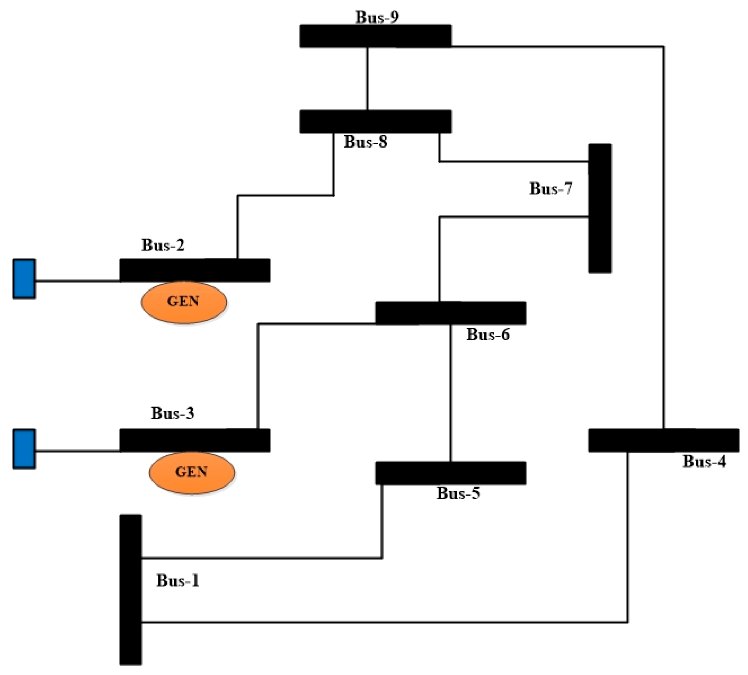
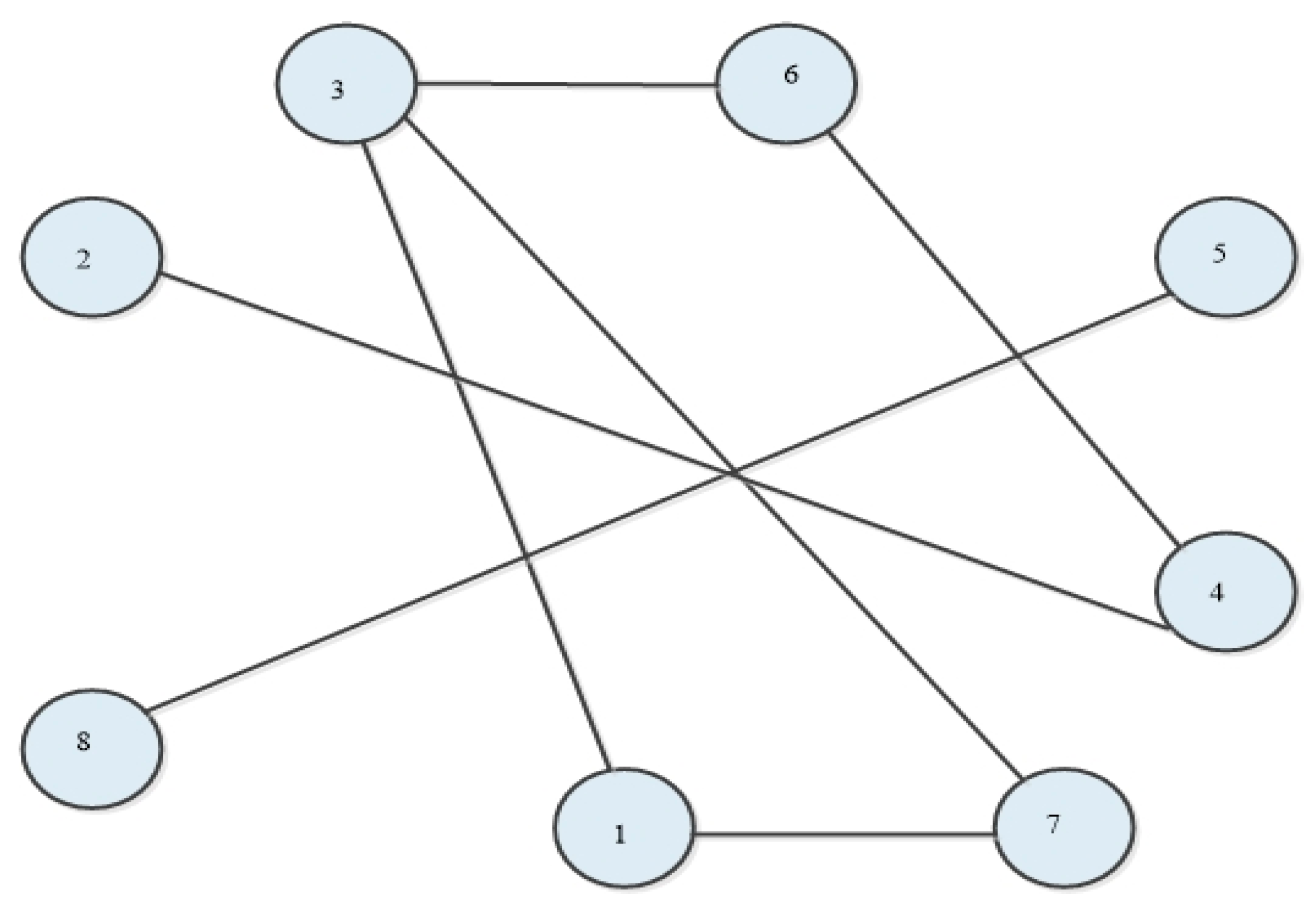
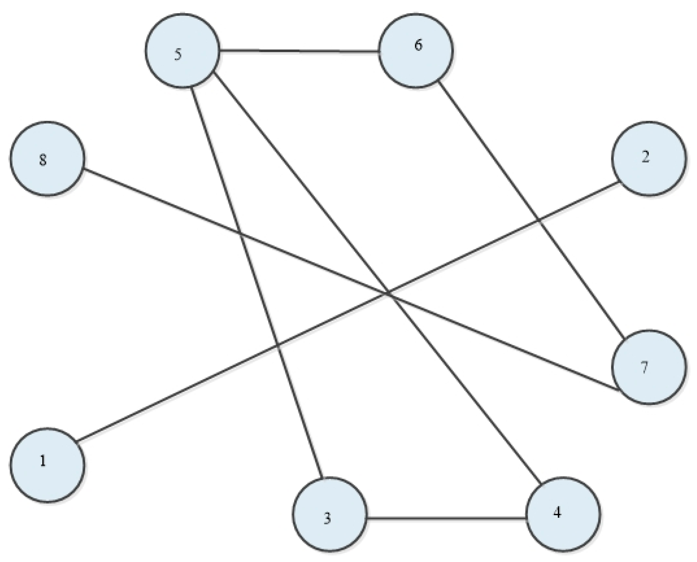
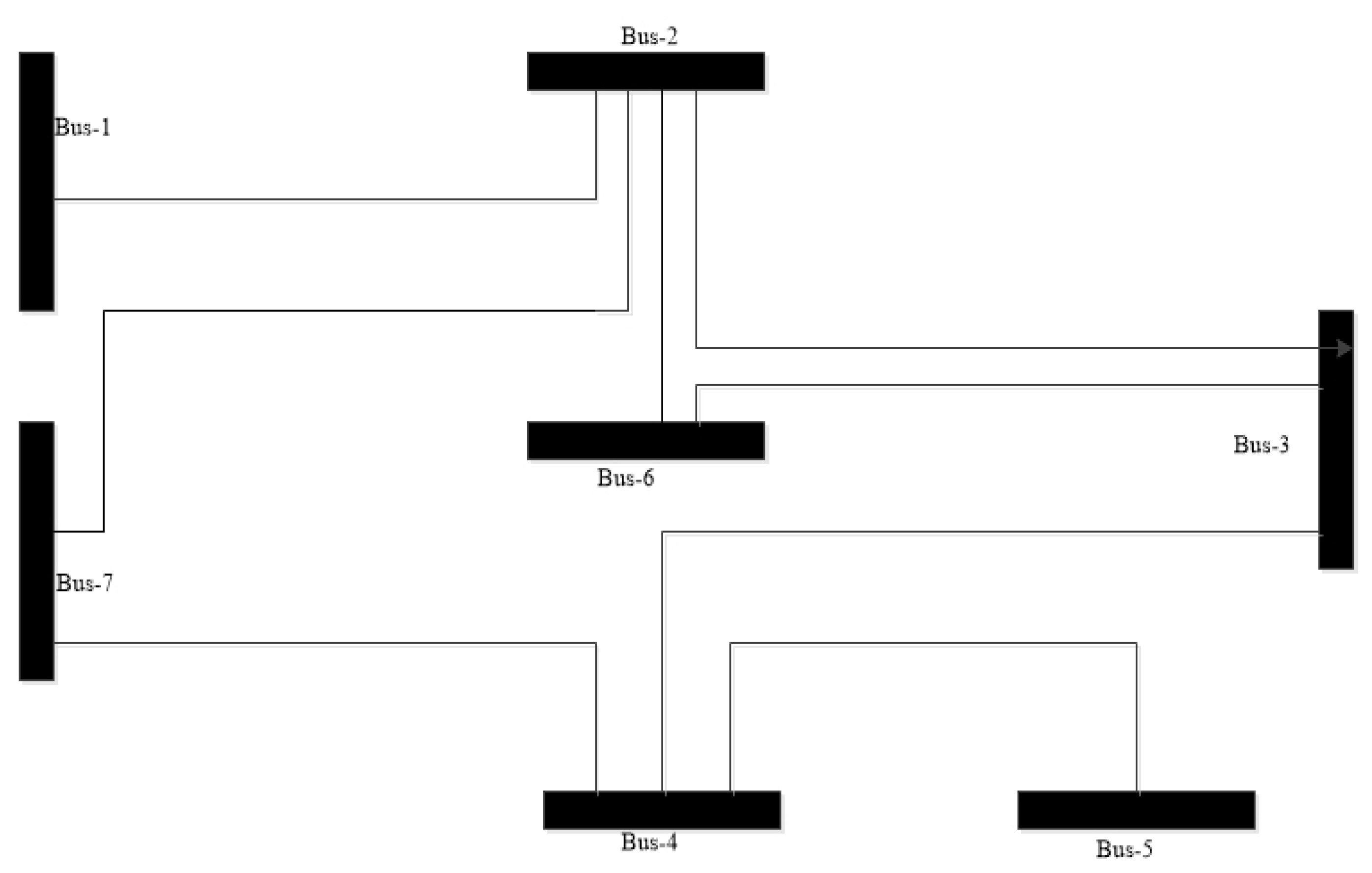
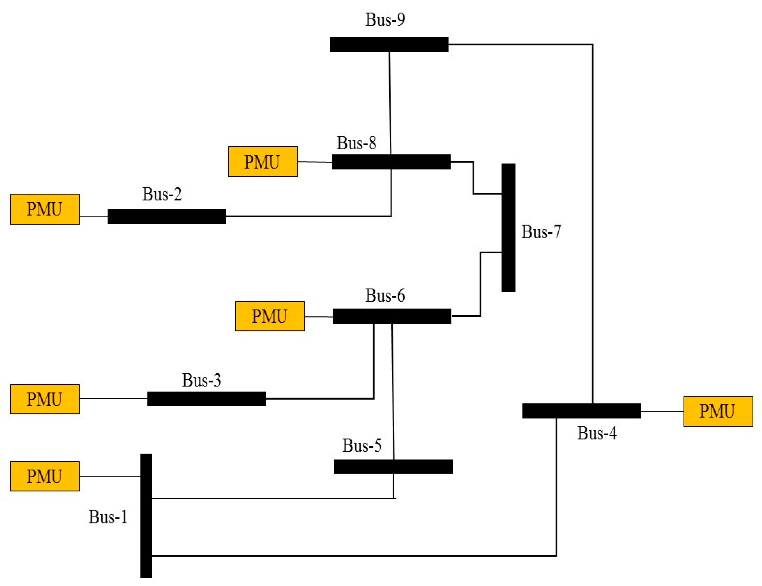
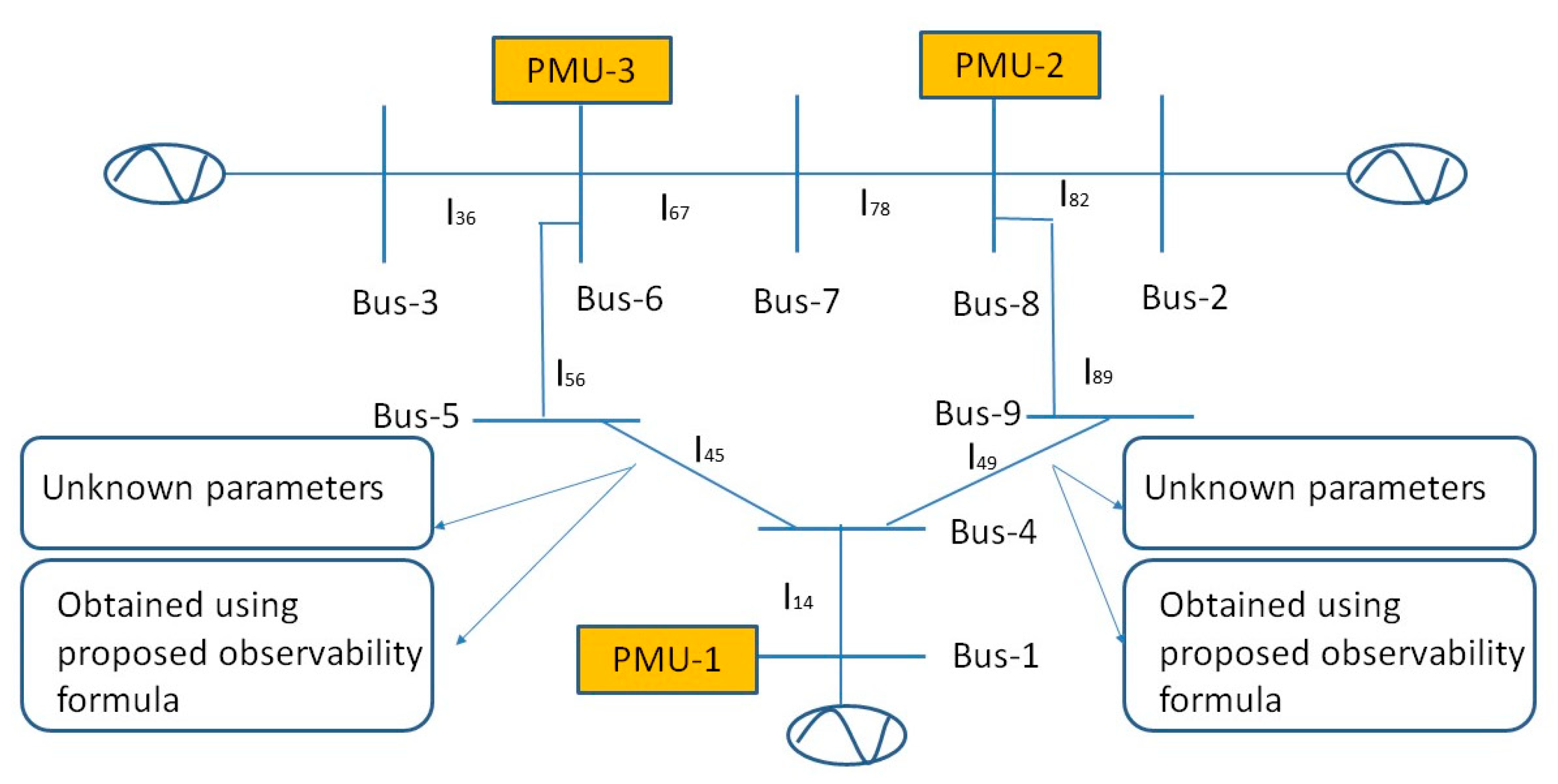
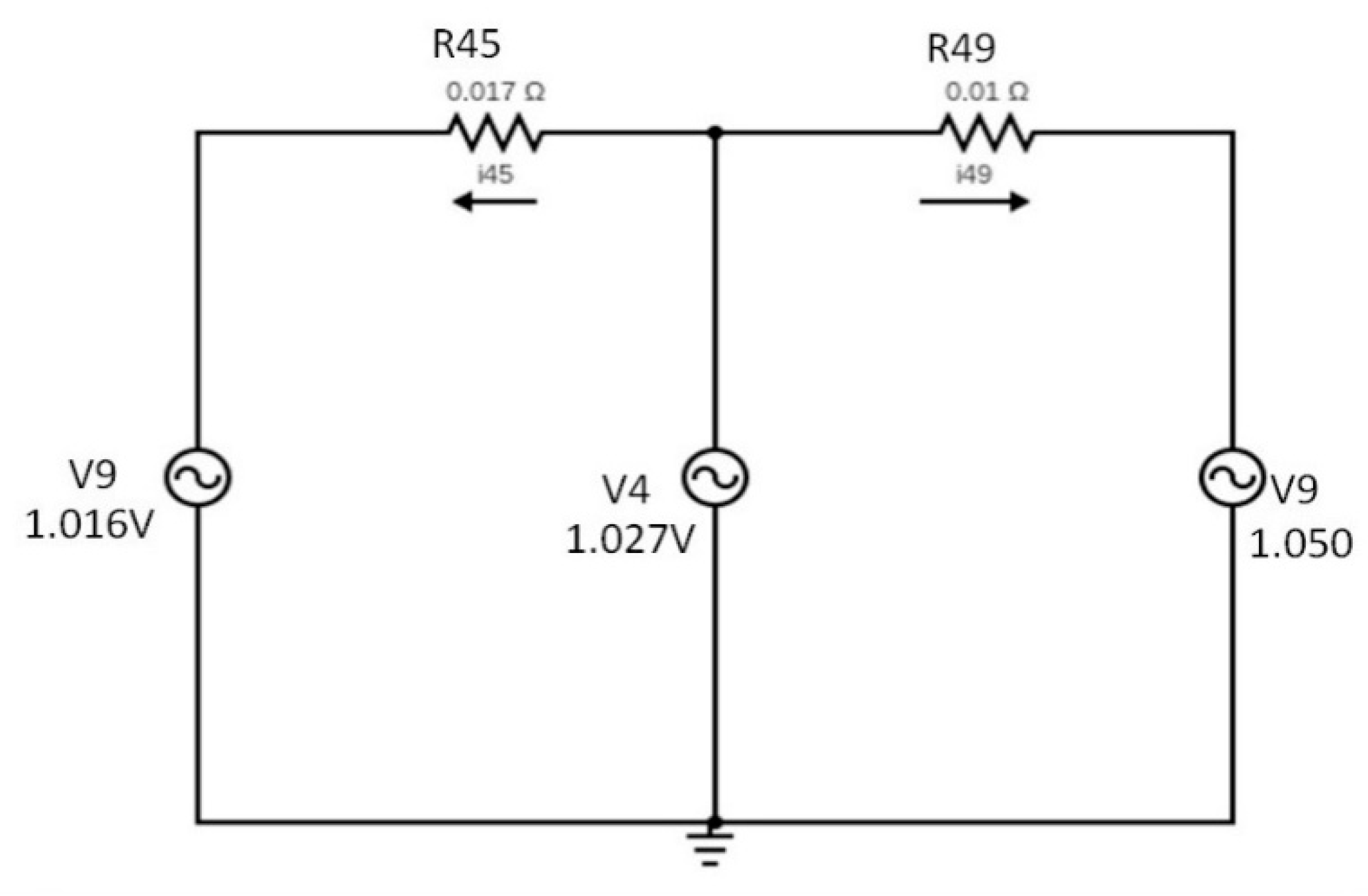
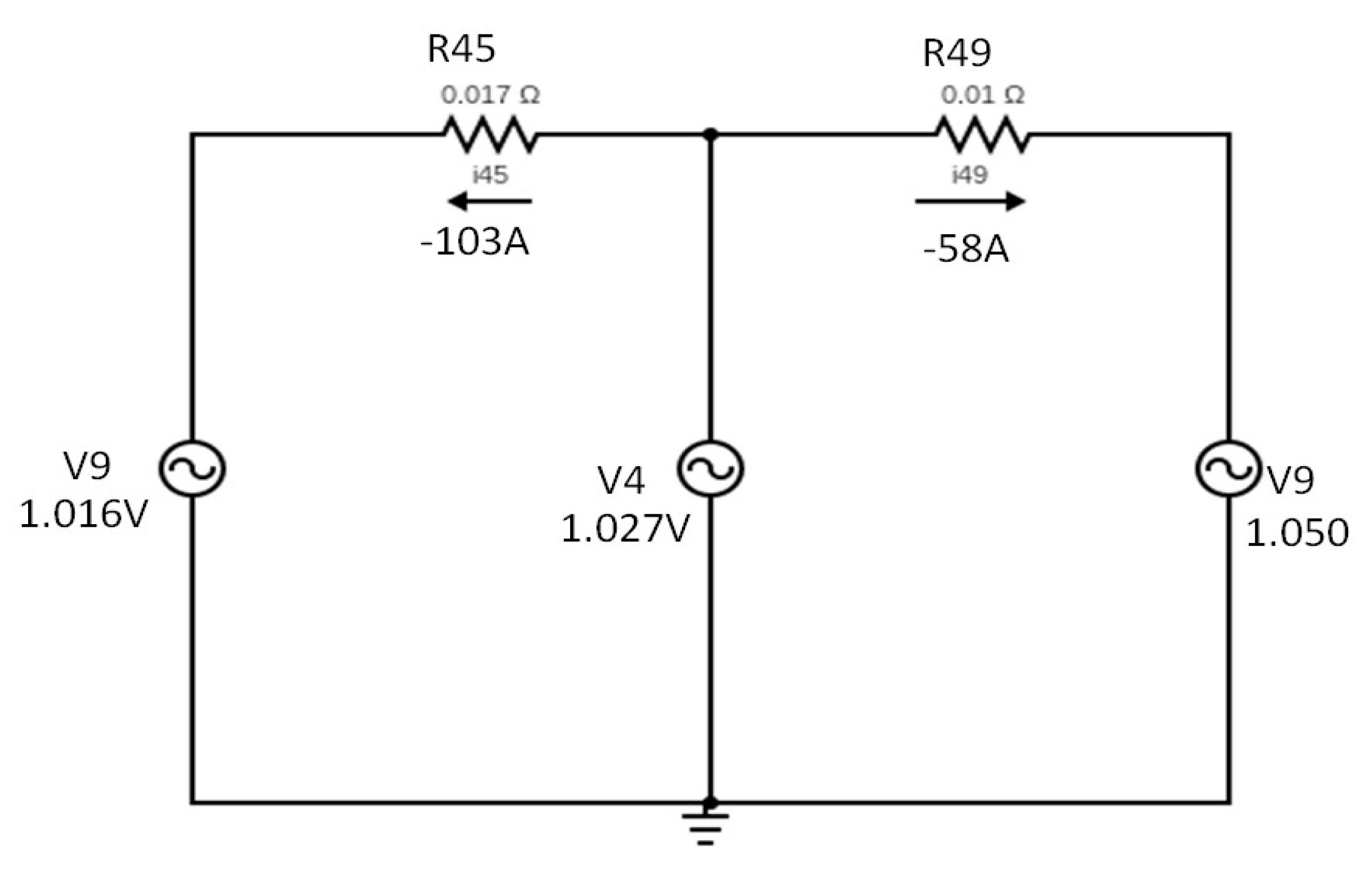
3.2. PMU Allocation on IEEE-Network Topology through Proposed Modeling

A graphical representation of the PMU allocations on the IEEE- bus networks is given in this section. The proposed PMU placement topology on the IEEE-network has been calculated through the proposed OPP problem modeling, and the voltage and current phasor calculation of the network has been carried out using the OPP problem standard observability equations. An illustration of the IEEE-9 bus network using the proposed OPP problem modeling with PMU allocations and the parameters calculations are shown in Figure 6:

Figure 6 shows the IEEE-9 bus network with the assigned PMU placement using the proposed modeling. Figure 6 shows the proposed results of optimum PMU placement in the IEEE-9 bus network using the case factor PMU channel limits. The illustration of the IEEE-network topology with PMU placement demonstrates the obtained proposed results. Three PMUs are assigned to bus-1, bus-6, and bus-8, which cover the parameters of the IEEE-9 bus network, and the remaining parameters are calculated by OPP problem observability analysis. In the given IEEE-9 bus network, all the connected lines and voltage phasors are covered with the installed PMUs, but the branch line between buses 4 and 5 and buses 4 and 9, which is I₄₅ and I₄₉, are left because of the PMU connection with the neighboring nodes and their branches. However, with the help of the power flow analysis on the IEEE-9 bus network, observation using the proposed Kirchoff Voltage and Current Law (KVL/KCL) and Ohm’s law of the remaining parameters becomes possible. A power flow report on the IEEE-9 bus network using the Power System Analysis Toolbox is shown in Figure 7.

The Newton–Raphson method is used to solve the power flow analysis of the IEEE-9 bus network in order to acquire information regarding all the network parameters. After different iterations, the power flow report is completed in 0.24 s, and it is considered the optimum report to use for the unknown parameters of branch lines I₄₅ and I₄₉ of the IEEE-9 bus network by the proposed methodology. In Figure 8, the direct connections of the PMUs with the voltages and current lines are obtained from the power flow analysis on the IEEE-9 bus network

The remaining current lines, which are I₄₅ and I₄₉, are estimated through the proposed KCL approach using observability analysis and are calculated as:

$$I_{45}=V_4-V_5/R_{45}$$

(15)

$$I_{49}=V_4-V_9/R_{49}$$

(16)

$$I_{45}=-103.973 \mathrm{A}$$

(17)

$$I_{49}=-58.7 \mathrm{A}$$

(18)

The above equations explain how to find the parameters for the unknown incident branches using observability rules because the PMU directly measures the voltage phasors of the installed bus and current lines connected to that installed bus. In this case factor of PMU channel limits, three PMUs are deployed on busbars 1, 6, and 8, which cover all the network parameters except I₄₅ and I₄₉. Therefore, based on the PMU standard observability analysis and proposed KCL formulation, observability became possible on the unknown parameter area of the network.

Figure 9 is the resultant circuit diagram of the IEEE-9 bus network and is derived from the proposed observability KCL.

4. Conclusions

• This paper presents a newly proposed methodology to solve the OPP problem based on multiple objectives such as the removal of unwanted nodes from the placement sets, PMU channel limits, and single PMUs outage. Prior literature has not taken PTNs into account in their simulation results as there is no benefit in selecting it as an optimum PMU location because no power injection nor power is flowing through it and it cannot give observability coverage to other buses in a network. Thus, the focal point of the conducted work is to remove the PTNs from the optimum PMU placement sets. In a case consideration of channel limits, the optimal PMU placement is calculated by assigning the number of channels to the PMU device. The different numbers of PMU sets are obtained on every channel limit, which further describes the branch combinations of every channel limit. It has been noticed that the greater the number of PMU channels, the lower will be the number of PMUs required.
• A single PMU outage is another factor considered by the proposed methodology, in which it is stated that at least two PMUs must be installed on a single busbar to give coverage when one PMU becomes out of order. When a single busbar is observed by more than one PMU, it increases the measurement redundancy of that bus and defines the values of BOI and SORI. The current limitation of the proposed work are that it only works on an IEEE-standard datasets from MATPOWER, which is an open-source tool for electrical power system simulation and optimization. The obtained datasets range from small to large systems such as IEEE-9, 14, 24, 30, 39, 57, and 118 bus systems. Additionally, the proposed design is implemented on IEEE-datasets from MATPOWER on MATLAB Simulink-based software. The design will furtherly be extended to a larger area network with power flow analysis using IEEE-datasets, which can be useful when considering it in real-life practical situations, such as smart grid execution, conventional distribution power stations, error finding in the power supply, improving the performance of state estimations using fault detection, and smart metering systems.

References

1. Gayatri, M.T.L.; Sarma, A.V.R.S. Fast Initial State Assessment for State Estimator using Optimally Located Phasor Measurement Units. Int. J. Comput. Appl. 2012, 50, 24–28. [Google Scholar]
2. Baba, M.; Nor, N.B.; Ibrahim, T.B.; Sheikh, M.A. A comprehensive review for optimal placement of phasor measurement unit for network observability. Indones. J. Electr. Eng. Comput. Sci. 2020, 19, 301–308. [Google Scholar] [CrossRef]
3. Al-Badi, A.H.; Ahshan, R.; Hosseinzadeh, N.; Ghorbani, R.; Hossain, E. Survey of smart grid concepts and technological demonstrations worldwide emphasizing the Oman perspective. Appl. Syst. Innov. 2020, 3, 5. [Google Scholar] [CrossRef] [Green Version]
4. Gomez-Exposito, A.; Abur AGomez-Exposito, A.; Abur, A. Power System State Estimation: Theory and Implementation; CRC Press: Boca Raton, FL, USA, 2004; Volume 9, pp. 101–108. [Google Scholar]
5. Sun, L.; Chen, T.; Chen, X.; Ho, W.K.; Ling, K.V.; Tseng, K.J.; Amaratunga, G.A.J. Optimum Placement of Phasor Measurement Units in Power Systems. IEEE Trans. Instrum. Meas. 2019, 68, 421–429. [Google Scholar] [CrossRef]
6. Chen, J.; Member, S.; Abur, A. Placement of PMUs to Enable Bad Data Detection in State Estimation. IEEE Trans. Power Syst. 2006, 21, 1608–1615. [Google Scholar] [CrossRef]
7. Baba, M.; Nor, N.; Irfan, M.; Tahir, M. A Strategic and Significant Method for the Optimal Placement of Phasor Measurement Unit for Power System Network. Symmetry 2020, 12, 1174. [Google Scholar] [CrossRef]
8. Bei, X.; Yoon, Y.J.; Abur, A. Optimal Placement and Utilization of Phasor Measurements for State Estimation; PSERC Publication: Ithaca, NY, USA, 2005; Volume 1. [Google Scholar]
9. Chakrabarti, S.; Kyriakides, E. Placement of Synchronized Measurements for Power System Observability. IEEE Trans. Power Deliv. 2009, 24, 12–19. [Google Scholar] [CrossRef] [Green Version]
10. Zhou, M.; Member, I.S.; Centeno, V.A.; Member, I.S.; Novosel, D.; Fellow, I.; Volskis, H.A.R. A Preprocessing Method for Effective PMU Placement Studies. In Proceedings of the 2008 Third International Conference on Electric Utility Deregulation and Restructuring and Power Technologies, Nanjing, China, 6–9 April 2008; pp. 2862–2867. [Google Scholar]
11. Dua, D.; Dambhare, S.; Gajbhiye, R.K.; Member, S.; Soman, S.A. Optimal Multistage Scheduling of PMU Placement: An ILP Approach. IEEE Trans. Power Deliv. 2008, 23, 1812–1820. [Google Scholar] [CrossRef]
12. Farsadi, M.; Golahmadi, H.; Shojaei, H. Phasor Measurement Unit (PMU) allocation in power system with different algorithms. In Proceedings of the 2009 International Conference on Electrical and Electronics Engineering-ELECO 2009, Bursa, Turkey, 5–8 November 2009; pp. 396–400. [Google Scholar] [CrossRef]
13. Peng, C.; Sun, H.; Guo, J. Multi-objective optimal PMU placement using a non-dominated sorting differential evolution algorithm. Int. J. Electr. Power Energy Syst. 2010, 32, 886–892. [Google Scholar] [CrossRef]
14. Gavrilaş, M.; Rusu, I.; Gavrilaş, G.; Ivanov, O. Synchronized phasor measurements for state estimation. Electrotech. Et Electroenerg. 2008, 335–344. [Google Scholar]
15. Yang, Y.; Shu, H.; Yue, L. Engineering Practical Method for PMU Placement of 2010 Yunnan power grid in China. In Proceedings of the 2009 International Conference on Sustainable Power Generation and Supply, Nanjing, China, 6–7 April 2010; pp. 1–6. [Google Scholar] [CrossRef]
16. Su, C.; Chen, Z. Optimal placement of phasor measurement units with new considerations. In Proceedings of the 2010 Asia-Pacific Power and Energy Engineering Conference, Chengdu, China, 28–31 March 2010; pp. 1–4. [Google Scholar] [CrossRef]
17. Chakraborty, F.P. Moderna Therapeutics, Tirtha Chakraborty, Documents. (12). U.S. Patent 9.255,129 B2, February 2016. [Google Scholar]
18. Gou, B. Generalized Integer Linear Programming Formulation for Optimal PMU Placement. IEEE Trans. Power Syst. 2008, 23, 1099–1104. [Google Scholar] [CrossRef]
19. Phadke, A.G.; Thorp, J.S. History and applications of phasor measurements. In Proceedings of the 2006 IEEE PES Power Systems Conference and Exposition, Atlanta, GA, USA, 29 October–1 November 2006; pp. 331–335. [Google Scholar]
20. Xu, P.; Wollenberg, B.F. Power System Observability and Optimal Phasor Measurement Unit Placement; University of Minnesota: Minneapolis, MN, USA, 2015. [Google Scholar]
21. Azizi, S.; Dobakhshari, A.S.; Member, S.; Sarmadi, S.A.N. Optimal PMU Placement by an Equivalent Linear Formulation for Exhaustive Search. IEEE Trans. Smart Grid 2012, 3, 174–182. [Google Scholar] [CrossRef]
22. Theodorakatos, N.P.; Manousakis, N.M.; Korres, G.N. Optimal placement of PMUS in power systems using binary integer programming and genetic algorithm. In MedPower; IET: London, UK, 2014; pp. 1–6. [Google Scholar]
23. Mohammadi-Ivatloo, B. Optimal placement of PMUs for power system observability using topology-based formulated algorithm. J. Appl. Sci. 2009, 9, 2463–2468. [Google Scholar] [CrossRef]
24. Marín, F.J.; García-Lagos, F.; Joya, G.; Sandoval, F. Optimal phasor measurement unit placement using genetic algorithms. In International Work-Conference on Artificial Neural Networks; Springer: Berlin/Heidelberg, Germany, 2003; pp. 486–493. [Google Scholar]
25. Boisen, M.B. Power system observability with minimal phasor measurement placement—Power Systems. IEEE Trans. Power 1993, 8, 707–715. [Google Scholar]
26. Peng, J.; Sun, Y.; Wang, H.F. Optimal PMU placement for full network observability using Tabu search algorithm. Int. J. Electr. Power Energy Syst. 2006, 28, 223–231. [Google Scholar] [CrossRef]
27. Milošević, B.; Begović, M. Nondominated sorting genetic algorithm for optimal phasor measurement placement. IEEE Trans. Power Syst. 2003, 18, 69–75. [Google Scholar] [CrossRef]
28. Sadu, A.; Kumar, R.; Kavasseri, R.G. Optimal placement of Phasor Measurement Units using Particle swarm Optimization. In Proceedings of the 2009 World Congress on Nature & Biologically Inspired Computing (NaBIC), Coimbatore, India, 9–11 December 2009; pp. 1708–1713. [Google Scholar]
29. Chakrabarti, S.; Kyriakides, E. Optimal Placement of Phasor Measurement Units for Power System Observability. IEEE Trans. Power Syst. 2008, 23, 1433–1440. [Google Scholar] [CrossRef]
30. Abd Rahman, N.H.; Zobaa, A.F. Integrated mutation strategy with modified binary PSO algorithm for optimal PMUs placement. IEEE Trans. Ind. Inform. 2017, 13, 3124–3133. [Google Scholar] [CrossRef]
31. Zhong, J. Phasor Measurement Unit (PMU) Placement Optimisation in Power Transmission Network Based on Hybrid Approach. Master’s Thesis, RMIT University, Melbourne, Australia, 2012; pp. 559–563. [Google Scholar]
32. Jaiswal, V.; Thakur, S.S.; Mishra, B. Optimal placement of PMUs using Greedy Algorithm and state estimation. In Proceedings of the 2016 IEEE 1st International Conference on Power Electronics, Intelligent Control and Energy Systems (ICPEICES), Delhi, India, 4–6 July 2016; pp. 1–5. [Google Scholar]
33. Zimmerman, R.D.; Murillo-Sánchez, C.E.; Thomas, R.J. MATPOWER: Steady-state operations, planning, and analysis tools for power systems research and education. IEEE Trans. Power Syst. 2010, 26, 12–19. [Google Scholar] [CrossRef] [Green Version]
Figure 1. IEEE-9-Bus network [15].
Energies 14 05596 g001
Figure 2. Input Connectivity between the nodes in a graph.
Energies 14 05596 g002
Figure 3. Output Connectivity between the nodes in the graph.
Energies 14 05596 g003
Figure 4. Interconnected IEEE-7 buses network.
Energies 14 05596 g004
Figure 5. IEEE-9 bus network with additionally installed PMUs for PMUs outage.
Energies 14 05596 g005
Figure 6. IEEE-9 Bus network with PMU placement demonstrations and parameter calculations.
Energies 14 05596 g006
Figure 7. Power Flow Analysis Report of the IEEE-9 SLD.
Energies 14 05596 g007
Figure 8. Circuit Diagram of the unknown parameters of the IEEE-9 SLD.
Energies 14 05596 g008
Figure 9. Circuit Diagram of the known parameters of the IEEE-9 SLD.
Energies 14 05596 g009