A Distributionally Robust Chance-Constrained Unit Commitment with N-1 Security and Renewable Generation

Abstract

With the increasing penetration of renewable energy generation, one of the major challenges is the problem of how to express the stochastic process of wind power and photovoltaic output as the exact probability density and distribution, in order to improve the security and accuracy of unit commitment results, a distributed robust security-constrained optimization model based on moment uncertainty is proposed, in which the uncertainty of wind and photovoltaic power is captured by two uncertain sets of first- and second-order moments, respectively. The two sets contain the probability distribution of the forecast error of the wind and photovoltaic power, and in the model, the energy storage is considered. In order to solve the model effectively, firstly, based on the traditional chance-constrained second-order cone transformation, according to the first- and second-order moments polyhedron expression of the distribution set, a cutting plane method is proposed to solve the distributed robust chance constraints. Secondly, the modified IEEE-RTS 24 bus system is selected to establish a simulation example, an improved generalized Benders decomposition algorithm is developed to solve the model to optimality. The results show that the unit commitment results with different emphasis on economy and security can be obtained by setting different conservative coefficients and confidence levels and, then, provide a reasonable decision-making basis for dispatching operation.

1. Introduction

In recent years, the rapid growth of renewable energy represented by wind and photovoltaic power in the energy system has greatly reduced the consumption of fossil fuels and greenhouse gas emissions [1]. However, its uncertainty and intermittence have a great impact on the security and stable operation of the power system. Therefore, how to solve the problem of unit commitment with large scale wind and photovoltaic power uncertainty has become a research hotspot.

In many unit commitment (UC) models considering the uncertainty of renewable generation, the traditional UC adopts a simple and feasible standby capacity method to deal with the uncertainty of renewable generation. This method is simple and fast, but it is blind and arbitrary. As a common method to deal with data uncertainty in optimization problems, stochastic programming has been widely explored in the past decade [2,3,4,5,6]. It mainly includes chance constraint and conditional risk method. This kind of method not only has large calculation scale, but also needs to know the deterministic distribution of random variables. Another tool for optimization against uncertainty is robust optimization. This method seeks the optimal objective values of all possible worst-case scenarios in the uncertainty set. In references [7,8,9,10], a robust optimization model for different objective functions is proposed based on the modeling of uncertain load and renewable energy through an adjustable robust optimization framework. However, in view of the fact that the worst case involved does not always happen, the optimization results are too conservative or aggressive. As a compromise method, distributed robust optimization can be used to solve the limitations of stochastic programming and robust optimization. In reference [11], a moment-based distributed robust model for UC is established, and the linear decision rule approximation method is applied to solve the model. However, only the uncertainty of wind power is considered, the impact of energy storage is not considered. In reference [12], the occurrence of accidents is regarded as a random event, and the moment uncertainty robust optimization method of unit commitmentconstrained by emergency accidents is studied without considering the uncertainty of renewable energy. The distribution set of the first- and second-order moment of wind power forecast error is given in reference [13], and the model is transformed into a bilinear matrix inequality problem to solve. Reference [14] obtained the first- and second-order moment information of wind power forecast error based on historical experience data and, then, transformed the optimal power flow model into convex second-order cone programming to solve the problem. In the above methods [11,12,13,14], DC power flow is used to replace AC power flow approximately, without considering the influence of reactive power and node voltage on the optimization results. The operation strategy obtained on this basis may lead to the risk of under voltage or over voltage on some key buses of the system. Reference [15] proposes a stochastic unit commitment (SUC) model to avoid the load loss risk caused by wind power uncertainty. In reference [16], the uncertainty of wind power is represented by the scenario tree model. Such a scenario tree is constructed by considering several stages, and each time period has several hours. The uncertainty of wind power generation in each cycle is represented by some discrete branches. This technology is suitable for modeling the recourse behavior of generator and energy storage device when the system uncertainty is realized successively. Reference [17] proposes a transmission capacity margin assessment (TCMA) model. Using dual theory and linearization technology, the model is transformed into mixed integer linear programming (MILP). In reference [18], the control characteristics of wind power plants is summarized, and the ability of wind power plants to provide fast regulation and frequency response services was determined.

Considering that the prediction accuracy of wind and photovoltaic power cannot accurately describe its probability, stochastic or robust optimization, such as widely used approximate normal distribution [19], beta distribution [20], mixed Laplace distribution [21], Cauchy distribution [22], α-steady-state distribution [23], etc., are essentially approximate methods, which is difficult to maintain the effectiveness of decision making. Distributed robust optimization combines robust optimization and stochastic optimization, two excellent methods with risk decision making, to implement the scheduling strategy under the probability distribution scenario of the worst uncertainty in the fuzzy set. For example, distributed robust unit commitment decision [24,25], reserve scheduling [26], and optimal power flow [27] can improve the effectiveness of decision making. The construction form of fuzzy sets determines different conservatism and solution efficiency. At present, the commonly used distribution robust optimization method based on probability density function is based on the probability uncertainty of Monte Carlo sampling points [28], which retains the characteristics that the probability density function of long-term fitting is similar to that of short-term fitting. However, this method does not make full use of the moment of random variables, and the variable scale is huge, it is difficult to obtain its dual problem. In a long statistical period, the prediction error of wind and photovoltaic power follows a certain distribution [29,30]. However, in a short period of time, its distribution is similar to the determined distribution, but it is not exactly the same, that is, the moment of the probability distribution is also uncertain. The distributed robust optimization under moment uncertainty (DRO-MU) method recently studied in the field of mathematics [31] can consider the similar but different characteristics of long-term fitting of random variables [32].

Given the context above, a robust optimization model of UC distribution with AC power flow constraints based on uncertainty of wind and photovoltaic power forecast error moment is proposed. Considering the network security constraints, the coupling relationship among active power, reactive power, voltage, and phase angle is considered, and the collaborative optimization is carried out. By setting conservative coefficient and confidence level, the optimal UC results with different emphasis on economy and security can be obtained, which can provide reasonable decision-making basis for dispatching operation. the main contributions of this paper are as follows: we develop a moment-based distributionally robust chance-constrained unit commitment with N-1 security and renewable generation model, while considering AC optimal power flow (OPF) and energy storage constraints; by considering an ambiguity set including the first- and second-order moment information obtained from empirical data, the wind and solar generation uncertainties are properly modeled.

The remainder of this paper is structured as follows. Section 2 first provides preliminaries on expansion time horizon and uncertainty modeling and, then, presents the proposed distributionally robust chance-constrained unit commitment (DRCCUC) model. Section 3 explains the solution methodology. Section 4 provides a comprehensive case study based on the IEEE RTS-24 node test system. Section 5 concludes the paper.

2. Distributed Robust Unit Commitment Model

2.1. Wind and Photovoltaic Fluctuations

In this paper, the active power output of each wind farm and photovoltaic power station is regarded as the sum of forecast value and forecast error value. The forecast value is regarded as the determined variable, and the forecast error value is treated as a random variable. It is assumed that the forecast error of all wind and photovoltaic power follow the normal distribution with zero mean value and are independent of each other [14]. For each wind farm, the hourly power is expressed as $P_{b,t}^{\mathrm{W}}+{\mathit{\omega }}_{b,t}^{\mathrm{W}}$, where $P_{b,t}^{\mathrm{W}}$ is the forecast active power of wind farm at bus b at time t, and ${\mathit{\omega }}_{b,t}^{\mathrm{W}}$ is the forecast error of active power of wind farm at bus b at time t. For each photovoltaic power station, the hourly output is expressed as $P_{b,t}^{\mathrm{PV}}+{\mathit{\omega }}_{b,t}^{\mathrm{PV}}$, where $P_{b,t}^{\mathrm{PV}}$ is the forecast active power of photovoltaic power station at bus b at time t, and ${\mathit{\omega }}_{b,t}^{\mathrm{PV}}$ is the forecast error of active power of photovoltaic power station at bus b at time t. As the security operation of power system requires that the power generation and power consumption should always be balanced, any deviation of wind and photovoltaic power from the forecast value must be balanced through the adjustment of controllable power generation. Since the power injection of each bus is fluctuating, a control scheme is needed to ensure that the power generation is always equal to the demand within a given time window. In this paper, it is assumed that all the generators participating in the control respond in a proportional manner to the fluctuation of the generalized load (assuming the forecast actual load minus the random wind and photovoltaic power), but the proportional coefficients may be different. Therefore, we call it initial value joint result frequency control and quadratic frequency control affine control. In this paper, the adjustment of wind and photovoltaic power fluctuation is modeled as an affine control strategy, and the activation of generation reserve is controlled by automatic generation control (AGC). The power balance is established in tens of seconds by AGC as follows:

$${\widehat{P}}_{i,t}=P_{i,t}-{\alpha }_{i,t}^{}{\mathbf{\Omega }}_t\hspace{1em}\forall t\in T, i\in G$$

(1)

$${\mathbf{\Omega }}_{ t}={\mathbf{\Omega }}_{ t}^{\mathrm{W} }+{\mathbf{\Omega }}_{ t}^{\mathrm{PV}}; {\mathbf{\Omega }}_{ t}^{\mathrm{W} }={\displaystyle \sum _{w=1}^W{\mathit{\omega }}_{w,t}^{\mathrm{W}}}; {\mathbf{\Omega }}_{ t}^{\mathrm{PV}}={\displaystyle \sum _{pv=1}^{PV}{\mathit{\omega }}_{pv,t}^{\mathrm{PV}}}$$

(2)

where $G$ is the number of generators; $W$ is the number of wind farms; $PV$ is the number of photovoltaic power stations; $T$ is the scheduling cycle and the time interval is 1 h; $P_{i,t}$ is active power of generator; ${\alpha }_{i,t}^{}$ is participation coefficient of AGC controlled generator; ${\mathbf{\Omega }}_{ t}$ is the sum of forecast errors of output power of all wind farms and photovoltaic power stations; ${\mathbf{\Omega }}_{ t}^{\mathrm{W} }$ is all wind farm power forecast error; ${\mathbf{\Omega }}_{ t}^{\mathrm{PV}}$ is all power forecast error of photovoltaic power station. When ${\alpha }_{i,t}^{}$ is constant or equal in the scheduling period, the calculation processability of the unit commitment model will be significantly improved. However, it is taken as an optimization variable in this paper for economically advantageous. In practical application, because of the randomness and inaccuracy of wind speed, usually only part of the probability distribution information can be obtained. Therefore, this paper uses two uncertainty intervals to describe the uncertainty of wind and photovoltaic power forecast error, $\left[-{\overline{\mathit{\mu }}}_b^{\mathrm{w}},{\overline{\mathit{\mu }}}_b^{\mathrm{w}}\right]$ and $\left[-{\overline{\mathit{\mu }}}_b^{\mathrm{pv}},{\overline{\mathit{\mu }}}_b^{\mathrm{pv}}\right]$ represent the mean change interval of wind and photovoltaic power forecast error at the bus b, and $\left[{({\mathit{\sigma }}_b^{\mathrm{w}})}^2-{({\overline{\mathit{\sigma }}}_b^{\mathrm{w}})}^2,{({\mathit{\sigma }}_b^{\mathrm{w}})}^2+{({\overline{\mathit{\sigma }}}_b^{\mathrm{w}})}^2\right]$ and $\left[{({\mathit{\sigma }}_b^{\mathrm{pv}})}^2-{({\overline{\mathit{\sigma }}}_b^{\mathrm{pv}})}^2,{({\mathit{\sigma }}_b^{\mathrm{pv}})}^2+{({\overline{\mathit{\sigma }}}_b^{\mathrm{pv}})}^2\right]$ represent the variance change interval of wind and photovoltaic power forecast error at the bus and assume that the random variables of wind and photovoltaic power forecast error are independent of each other. In fact, there are several probability distribution functions whose mean value and variance are consistent with these information, then the fluctuation range of mean value and variance of wind and photovoltaic power is represented by polyhedron set as follows:

$$U_{\mathit{\mu }}=\left\{\begin{array}{r}\mathit{\mu }\in {ℝ}^{\left|W+PV\right|}:\left|{\mathit{\mu }}_b^{\mathrm{w}}+{\mathit{\mu }}_b^{\mathrm{pv}}\right|\le {\overline{\mathit{\mu }}}_b^{\mathrm{w}}+{\overline{\mathit{\mu }}}_b^{\mathrm{pv}}\\ {\displaystyle \sum _{b\in W+PV}\frac{\left|{\mathit{\mu }}_b^{\mathrm{w}}+{\mathit{\mu }}_b^{\mathrm{pv}}\right|}{{\overline{\mathit{\mu }}}_b^{\mathrm{w}}+{\overline{\mathit{\mu }}}_b^{\mathrm{pv}}}}\le {\mathsf{\Gamma }}_{\mathit{\mu }}\left|W+PV\right|\end{array}\right\}$$

(3)

$$U_{{\mathit{\sigma }}^2}=\left\{\begin{array}{r}{\mathit{\sigma }}^2\in {ℝ}^{\left|W+PV\right|}\\ \left|{({\mathit{\sigma }}_b^{\mathrm{w}})}^2+{({\mathit{\sigma }}_b^{\mathrm{pv}})}^2\right|\le {({\overline{\mathit{\sigma }}}_b^{\mathrm{w}})}^2+{({\overline{\mathit{\sigma }}}_b^{\mathrm{pv}})}^2\\ {\displaystyle \sum _{b\in W+PV}\frac{\left|{({\mathit{\sigma }}_b^{\mathrm{w}})}^2+{({\mathit{\sigma }}_b^{\mathrm{pv}})}^2\right|}{{({\overline{\mathit{\sigma }}}_b^{\mathrm{w}})}^2+{({\overline{\mathit{\sigma }}}_b^{\mathrm{pv}})}^2}}\le {\mathsf{\Gamma }}_{\mathit{\sigma }}\left|W+PV\right|\\ \end{array}\right\}$$

(4)

where ${\mathit{\mu }}_b^{\mathrm{w}}$ and ${\mathit{\mu }}_b^{\mathrm{pv}}$ are the mean variation of wind and photovoltaic power forecast error at bus b, respectively; ${\overline{\mathit{\mu }}}_b^{\mathrm{w}}$ and ${\overline{\mathit{\mu }}}_b^{\mathrm{pv}}$ are the upper limit of mean value change in wind and photovoltaic power forecast error at bus b, respectively; ${\mathsf{\Gamma }}_{\mathit{\mu }}$ is the mean interval conservative coefficient (the range limiting parameter of uncertainty set); ${\overline{\mathit{\sigma }}}_b^{\mathrm{w}}$ and ${\overline{\mathit{\sigma }}}_b^{\mathrm{pv}}$ are the upper limit of forecast error variance of wind and photovoltaic power at bus b, respectively; ${\mathsf{\Gamma }}_{\mathit{\sigma }}$ is the conservative coefficient of variance interval.

2.2. DRCCUC Model

The objective function of DRCCUC minimizes the operation cost of generator, including no-load cost, start-up cost, shutdown cost, fuel cost, spinning reserve cost, and emergency reserve cost.

$$\begin{array}{r}\min {\displaystyle \sum _{i=1}^G{\displaystyle \sum _{t=1}^T\{c_i^0\cdot x_{i,t}^{}+{\displaystyle \sum _{k\in K}{c}_i^k\cdot P_{i,t}^k}+C_{i,t}^{\mathrm{U}}+}}{C}_{i,t}^{\mathrm{D}}+\\ [c_i^{\mathrm{r}}\cdot (R_{i,t}^{+}+R_{i,t}^{-})+c_i^{*}\cdot R_{i,t}^{*}]+{\displaystyle \sum _{w=1}^W{\displaystyle \sum _{t=1}^T{C}_{w,t}^{\mathrm{W}}}}+{\displaystyle \sum _{pv=1}^{PV}{\displaystyle \sum _{t=1}^T{C}_{pv,t}^{\mathrm{PV}}}}\}\end{array}$$

(5)

where $c_i^0$ is no load cost of generator; $x_{i,t}^{}$ is the binary variable of generator start and stop state; $c_i^k$ is the section k (k = 1, 2, 3) rate for the unit fuel cost function; $P_{i,t}^k$ is the active power of section k for the fuel cost function of generator; $C_{i,t}^{\mathrm{U}}$ is the cost of generator start-up; $C_{i,t}^{\mathrm{D}}$ is the cost of generator shutdown; $c_i^{\mathrm{r}}$ is the spinning reserve cost for generators; $R_{i,t}^{+}$ is the positive spinning reserve of generator; $R_{i,t}^{-}$ is the negative spinning reserve of generator; $c_i^{*}$ is the contingency spinning reserve cost for generator accident; $R_{i,t}^{*}$ is the contingency spinning reserve of generator. $C_{w,t}^{\mathrm{W}}$ is the penalty cost of wind power spillage; $C_{pv,t}^{\mathrm{PV}}$ is the penalty cost of photovoltaic power spillage. The main constraints are formulated as follows:

$$y_{i,t}-z_{i,t}=x_{i,t}-x_{i,t-1}\hspace{1em}\forall t\in T,i\in G$$

(6)

$$y_{i,t}+z_{i,t}\le 1 \hspace{1em}\forall t\in T,i\in G$$

(7)

$$C_{i,t}^{\mathrm{U}}\ge C_i^{\mathrm{U}}\cdot \left(x_{i,t}-x_{i,t-1}\right) \mathrm{and} C_{i,t}^{\mathrm{U}}\ge 0\hspace{1em}\forall t\in T,i\in G$$

(8)

$$C_{i,t}^{\mathrm{D}}\ge C_i^{\mathrm{D}}\cdot \left(x_{i,t-1}-x_{i,t}\right) \mathrm{and} C_{i,t}^{\mathrm{D}}\ge 0\hspace{1em}\forall t\in T,i\in G$$

(9)

$$P_{i,t}-R_{i,t}^{-}\ge P_i^{\min }\cdot x_{i,t}\hspace{1em}\forall t\in T,i\in G$$

(10)

$$P_{i,t}+R_{i,t}^{+}+R_{i,t}^{*}\le P_i^{\max }\cdot x_{i,t}\hspace{1em}\forall t\in T,i\in G$$

(11)

$${\displaystyle \sum _{i=1}^G{\alpha }_{i,t}=1, 0\le {\alpha }_{i,t}\le x_{i,t}}\hspace{1em}\forall i\in G,t\in T$$

(12)

$${\displaystyle \sum _{i=G_r}^{}{\alpha }_{i,t}}={\delta }_{r,t}={\theta }_{r,t}=0\hspace{1em}\forall t\in T$$

(13)

$${\displaystyle \sum _{\begin{array}{l}{b}^{\prime }\in B\\ b^{\prime }\ne r\end{array}}^{}{Y}_{b,b^{\prime }}\cdot {\delta }_{b^{\prime },t}}={\displaystyle \sum _{i\in G_b}^{}{\alpha }_{i,t}}\hspace{1em}\forall b\in B,t\in T$$

(14)

$$P_{i,t}^{gc}=P_{i,t}+{\widehat{P}}_{i,t}^{gc}\hspace{1em}\forall t\in T, i,gc\in G$$

(15)

$${\widehat{P}}_{i,t}^{gc}\le R_{i,t}^{*}, {\displaystyle \sum _{i=1}^G{\widehat{P}}_{i,t}^{gc}}=0, {\widehat{P}}_{gc,t}^{gc}=-P_{gc,t}\hspace{1em}\forall t\in T; i,gc\in G$$

(16)

$$\underset{W,PV~U\left(\mathit{\mu },{\mathit{\sigma }}^2\right)}{\mathrm{Pr}}\left(R_{i,t}^{-}\ge {\mathbf{\Omega }}_t{\alpha }_i^t\right)\le 1-{\epsilon }_i^{\mathrm{G}}\hspace{1em}\forall \mathit{\mu }\in U_{\mathit{\mu }},{\mathit{\sigma }}^2\in U_{{\mathit{\sigma }}^2}$$

(17)

$$\underset{W,PV~U\left(\mathit{\mu },{\mathit{\sigma }}^2\right)}{\mathrm{Pr}}\left(R_{i,t}^{+}\ge -{\mathbf{\Omega }}_t{\alpha }_i^t\right)\le 1-{\epsilon }_i^{\mathrm{G}}\hspace{1em}\forall \mathit{\mu }\in U_{\mathit{\mu }},{\mathit{\sigma }}^2\in U_{{\mathit{\sigma }}^2}$$

(18)

where $y_{i,t}$ is the binary variable of generator starting state; $z_{i,t}$ is a binary variable of generator shutdown state; $C_i^{\mathrm{U}}$ is the cost of generator start-up; $C_i^{\mathrm{D}}$ is the Cost of generator shutdown; Constraint (6) according to the start-up and stop state between t hour and t − 1 determines whether the generator is in the start-up or stop state at t hour; Constraint (7) ensures that start-up and shut-down of any generator will not occur at the same time. $P_i^{\min }$ and $P_i^{\max }$ are the minimum and maximum active power of generator, respectively; ${\theta }_{r,t}$ is the reference bus voltage phase angle; ${\delta }_{r,t}$ is an auxiliary variable; ${\widehat{P}}_{i,t}^{gc}$ is the increased active power of generator in case of generator fault. In order to ensure the power balance, Constraint (16) forces the generator to stop unexpectedly, and the power output change is equal to its pre accident power output; $\mathrm{Pr}()$ represents the probability of occurrence of random events; ${\epsilon }_i^{\mathrm{G}}$ indicates the probability of insufficient reserve capacity of generator; Constraints (10) and (11) constrain the positive and negative rotating reserve and emergency reserve capacity of the generator; Constraints (17) and (18) ensure that the generator emergency reserve capacity is greater than the expected reserve activation. The combination of Constraints (11) and (16) can ensure that the total accident reserve is sufficient to cover any generator shutdown. Constraints (17) and (18) are robust chance constraints on the distribution of generator reserve capacity. Constraint (12) limits the number of generators participating in the automatic generation control based on the on–off state.

$$x_{i,t}^{}\le x_{i,0}\hspace{1em}\forall t\le t_i^{\mathrm{on}}+t_i^{\mathrm{off}}, i\in G$$

(19)

$${\displaystyle \sum _{t=\overline{t}}^t{y}_{i,t}}\le x_{i,t}\hspace{1em}\forall t\ge t_i^{\mathrm{on}}, \overline{t}=t-t_i^{\min \mathrm{on}}+1, i\in G$$

(20)

$${\displaystyle \sum _{t=\underset{\_}{t}}^t{z}_{i,t}}\le 1-x_{i,t}\hspace{1em}\forall t\ge t_i^{\mathrm{off}}, \underset{\_}{t}=t-t_i^{\min \mathrm{off}}+1, i\in G$$

(21)

$$P_i^{\mathrm{down}}\ge P_{i,t-1}-P_{i,t}\hspace{1em}\forall t\in T, i\in G$$

(22)

$$P_i^{\mathrm{up}}\ge P_{i,t}-P_{i,t-1}\hspace{1em}\forall t\in T, i\in G$$

(23)

Constraints (19)–(23) are the minimum start-up and shutdown time and climbing constraints of the generator, where $t_i^{\mathrm{on}}$ is the accumulated running time of the generator from t = 0; $t_i^{\mathrm{off}}$ is the accumulated shutdown time of generator from t = 0; $t_i^{\min \mathrm{on}}$ is the minimum allowable operation time of generator; $t_i^{\min \mathrm{off}}$ is the minimum allowable shutdown time of generator; $P_i^{\mathrm{up}}$ is the generator active output rise rate limit; $P_i^{\mathrm{down}}$ is the generator active power output reduction rate limit. Equation (19) constrains the switching state of the generator under initial conditions; Equations (20) and (21) are the constraints of minimum starting time and minimum stopping time of generator; Equations (22) and (23) are generator ramp constraints.

$$F_{m,n,t}^{}={\beta }_{m,n}^{}\cdot ({\theta }_{m,t}^{}-{\theta }_{n,t}^{}), \left|F_{m,n,t}^{}\right|\le F_{m,n}^{\mathrm{MAX}}\hspace{1em}\forall \{m,n\}\in L$$

(24)

$$\begin{array}{r}{\displaystyle \sum _{b^{\prime }\in B}^{}{Y}_{b,b^{\prime }}^{}\cdot }{\theta }_{b^{\prime },t}^{}={\displaystyle \sum _{i\in G_b}^{}{P}_{i,t}}+P_{b,t}^{\mathrm{W}}+{\mathit{\omega }}_{b,t}^{\mathrm{w}}+P_{b,t}^{\mathrm{PV}}+\\ {\mathit{\omega }}_{b,t}^{\mathrm{pv}}-P_{b,t}^{\mathrm{D}}+P_{b,t}^{\mathrm{DIS}}-P_{b,t}^{\mathrm{CH}}\hspace{1em}\forall b\in B,t\in T\end{array}$$

(25)

$$\begin{array}{r}\underset{W,PV~U\left(\mathit{\mu },{\mathit{\sigma }}^2\right)}{\mathrm{Pr}}(F_{m,n,t}^{}+{\beta }_{m,n}^{}\cdot {\mathbf{\Omega }}_t\cdot ({\delta }_{n,t}-{\delta }_{m,t})+\\ {\beta }_{m,n}^{}\cdot {\widehat{\mathit{\omega }}}_t^{\mathrm{W}}\cdot ({\pi }_{m,t}-{\pi }_{n,t})+{\beta }_{m,n}^{}\cdot {\widehat{\mathit{\omega }}}_t^{\mathrm{PV}}\cdot ({\pi }_{m,t}-{\pi }_{n,t})\\ \le F_{m,n}^{\mathrm{MAX}})\ge 1-{\epsilon }_l^{\mathrm{L}}\hspace{1em}\forall \{m,n\}\in L,\mathit{\mu }\in U_{\mathit{\mu }},{\mathit{\sigma }}^2\in U_{{\mathit{\sigma }}^2}\end{array}$$

(26)

$$\begin{array}{r}\underset{W,PV~U\left(\mathit{\mu },{\mathit{\sigma }}^2\right)}{\mathrm{Pr}}(F_{m,n,t}^{}+{\beta }_{m,n}^{}\cdot {\mathbf{\Omega }}_t\cdot ({\delta }_{n,t}-{\delta }_{m,t})+\\ {\beta }_{m,n}^{}\cdot {\widehat{\mathit{\omega }}}_t^{\mathrm{W}}\cdot ({\pi }_{m,t}-{\pi }_{n,t})+{\beta }_{m,n}^{}\cdot {\widehat{\mathit{\omega }}}_t^{\mathrm{PV}}\cdot ({\pi }_{m,t}-{\pi }_{n,t})\\ \ge -F_{m,n}^{\mathrm{MAX}})\ge 1-{\epsilon }_l^{\mathrm{L}}\hspace{1em}\forall \{m,n\}\in L,\mathit{\mu }\in U_{\mathit{\mu }},{\mathit{\sigma }}^2\in U_{{\mathit{\sigma }}^2} \end{array}$$

(27)

Equations (24)–(27) are DC power flow constraints under N state, where $F_{m,n,t}^{}$ is the active power flow of transmission line; ${\beta }_{m,n}^{}$ is the susceptance of the line; $F_{m,n}^{\mathrm{MAX}}$ is the maximum active power flow of transmission line; $P_{b,t}^{\mathrm{DIS}}$ is the active power of energy storage discharge; $P_{b,t}^{\mathrm{CH}}$ is the charging active power for energy storage; ${\pi }_{m,t}$ is the mth row of the inverse of the admittance matrix; ${\epsilon }_l^{\mathrm{L}}$ is the probability of power overrun in normal operation.

$$F_{m,n,t}^c={\beta }_{m,n}^{}\cdot ({\theta }_{m,t}^c-{\theta }_{n,t}^c)\hspace{1em}\forall \{m,n\}\in L$$

(28)

$$\begin{array}{r}{\displaystyle \sum _{b^{\prime }\in B}^{}{Y}_{b,b^{\prime }}^c\cdot }{\theta }_{b^{\prime },t}^c={\displaystyle \sum _{i\in G_b}^{}(P_{i,t}}+{\delta }_{i,t}^c)+P_{b,t}^{\mathrm{W}}+{\mathit{\omega }}_{b,t}^{\mathrm{w}}+P_{b,t}^{\mathrm{PV}}+\\ {\mathit{\omega }}_{b,t}^{\mathrm{pv}}-P_{b,t}^{\mathrm{D}}+P_{b,t}^{\mathrm{DIS}}-P_{b,t}^{\mathrm{CH}}\hspace{1em}\forall b\in B,t\in T\end{array}$$

(29)

$$\begin{array}{r}\underset{W,PV~U\left(\mathit{\mu },{\mathit{\sigma }}^2\right)}{\mathrm{Pr}}(F_{m,n,t}^c\le F_{m,n}^{\mathrm{MAX}})\ge 1-{\epsilon }_l^{\mathrm{LC}} \\ \forall \{m,n\}\in L,\mathit{\mu }\in U_{\mathit{\mu }},{\mathit{\sigma }}^2\in U_{{\mathit{\sigma }}^2} \end{array}$$

(30)

$$\begin{array}{r}\underset{W,PV~U\left(\mathit{\mu },{\mathit{\sigma }}^2\right)}{\mathrm{Pr}}(F_{m,n,t}^c\ge -F_{m,n}^{\mathrm{MAX}})\ge 1-{\epsilon }_l^{\mathrm{LC}} \\ \forall \{m,n\}\in L,\mathit{\mu }\in U_{\mathit{\mu }},{\mathit{\sigma }}^2\in U_{{\mathit{\sigma }}^2} \end{array}$$

(31)

Equations (28)–(31) are DC power flow constraints under N-1 state of generator and transmission line, where $F_{m,n,t}^c$ is the active power flow of transmission line in case of accident; ${\theta }_{m,t}^c$ is the bus phase angle in case of accident; ${\epsilon }_l^{\mathrm{LC}}$ is the probability of power overrun of transmission line in case of accident. Equations (26), (27), (30), and (31), respectively, represent the robust chance constraints of line power flow distribution under normal operation and accident conditions.

$$\begin{array}{r}{P}_{b,t}^{\mathrm{G}}+P_{b,t}^{\mathrm{W}}+P_{b,t}^{\mathrm{PV}}+P_{b,t}^{\mathrm{DIS}}-P_{b,t}^{\mathrm{CH}}-P_{b,t}^{\mathrm{D}}=\\ {\displaystyle \sum _{b^{\prime }\in b}^{}{V}_{b,t}{V}_{b^{\prime },t}\left(G_{b{b}^{\prime }}\cos {\theta }_{b{b}^{\prime },t}+B_{b{b}^{\prime }}\sin {\theta }_{b{b}^{\prime },t}\right)}\hspace{1em}\forall b,b^{\prime }\in B\end{array}$$

(32)

$$\begin{array}{r}{Q}_{b,t}^{\mathrm{G}}+Q_{b,t}^{\mathrm{W}}+Q_{b,t}^{\mathrm{PV}}-Q_{b,t}^{\mathrm{D}}=\\ {\displaystyle \sum _{b^{\prime }\in b}^{}{V}_{b,t}{V}_{b^{\prime },t}\left(G_{b{b}^{\prime }}\sin {\theta }_{b{b}^{\prime },t}-B_{b{b}^{\prime }}\cos {\theta }_{b{b}^{\prime },t}\right)}\hspace{1em}\forall b,b^{\prime }\in B\end{array}$$

(33)

$$V_b^{\mathrm{MIN}}\le V_{b,t}^{}\le V_b^{\mathrm{MAX}}\hspace{1em}\forall b\in B, t\in T$$

(34)

$$Q_i^{\mathrm{MIN}}\le Q_{i,t}^{}\le Q_i^{\mathrm{MAX}}\hspace{1em}\forall i\in G, t\in T$$

(35)

$${\left(F_{m,n,t}^{\mathrm{P}}\right)}^2+{\left(F_{m,n,t}^{\mathrm{Q}}\right)}^2\le {\left(F_{m,n,t}^{\mathrm{S}}\right)}^2\hspace{1em}\forall \{m,n\}\in L,t\in T$$

(36)

where $Q_{b,t}^{\mathrm{G}}$ is the reactive power of thermal power unit; $Q_{b,t}^{\mathrm{W}}$ is the reactive power of wind power; $Q_{b,t}^{\mathrm{V}}$ is the photovoltaic reactive power; $Q_{b,t}^{\mathrm{D}}$ is the reactive power of the load; $V_{b,t}$ is the node voltage amplitude; $G_{b{b}^{\prime }}$ is the real part of the bus admittance matrix; $B_{b{b}^{\prime }}$ is the imaginary part of node admittance matrix; $V_b^{\max }$ is the upper limit of node voltage amplitude; $V_b^{\min }$ is the lower limit of node voltage amplitude; $Q_{i,t}^{}$ is the reactive power output of thermal power units; $Q_i^{\max }$ is the upper limit of reactive power of thermal power unit; $Q_i^{\min }$ is the lower limits of reactive power of thermal power units; $F_{m,n,t}^{\mathrm{P}}$ and $F_{m,n,t}^{\mathrm{Q}}$ are the line active and reactive power; $F_{m,n,t}^{\mathrm{S}}$ is the line apparent power.

$$S_{es,t}^{\mathrm{CH}}+S_{es,t}^{\mathrm{DIS}}\le 1\hspace{1em}\forall es\in ES,t\in T$$

(37)

$$E_{es,t}=E_{es,t-1}+P_{es,t}^{\mathrm{CH}}\eta +P_{es,t}^{\mathrm{DIS}}/\eta \hspace{1em}\forall t\in T,es\in ES$$

(38)

$$0\le \eta P_{es,t}^{\mathrm{CH}}\le P_{es}^{\mathrm{MAX}}{S}_{es,t}^{\mathrm{CH}}\hspace{1em}\forall t\in T,es\in ES$$

(39)

$$0\le P_{es,t}^{\mathrm{DIS}}/\eta \le P_{es}^{\mathrm{MAX}}\left(1-S_{es,t}^{\mathrm{CH}}\right)\hspace{1em}\forall t\in T, es\in ES$$

(40)

$$0.1E_{es}^{\mathrm{MAX}}\le E_{es,t}\le 0.9E_{es}^{\mathrm{MAX}}\hspace{1em}\forall t\in T, es\in ES$$

(41)

where $S_{es,t}^{\mathrm{CH}}$ is the binary variable of energy storage charging state; $S_{es,t}^{\mathrm{DIS}}$ is the binary variable of energy storage discharge state; $E_{es,t}$ is the charge capacity of energy storage; $P_{es,t}^{\mathrm{CH}}$ and $P_{es,t}^{\mathrm{DIS}}$ are energy storage charging and discharging power, respectively; $\eta$ is the conversion efficiency of charging and discharging for energy storage; $P_{es}^{\mathrm{MAX}}$ and $E_{es}^{\mathrm{MAX}}$ are the maximum rated power and capacity of energy storage, respectively; Equation (37) is used to restrict the charging and discharging state of energy storage, Equation (38) is used to calculate the charging quantity of energy storage, Equations (39) and (40) restrict whether the energy storage can be charged and discharged at the same time, and Equation (41) restricts the upper and lower limits of charging quantity of energy storage.

3. Solution Methodology

Due to the nonconvex of distributed robust chance constraints and the strong nonlinearity of AC power flow equations, the large-scale mixed integer nonlinear programming (MINLP) model established in the previous section is difficult to solve directly by using existing commercial solvers. Among many UC solving algorithms, the general Benders decomposition (GBD) algorithm is widely used to solve MINLP problems. In order to improve the efficiency of traditional GBD, according to the basic idea of variable separation in reference [33], this paper proposes an improved GBD algorithm. Compared with traditional GBD, it is mainly reflected in the following two aspects: (1) an improved cut plane method for solving distributed robust chance constraints is proposed, which reduces the number of unnecessary iterations; (2) a network security constraint reduction method is proposed. Through a large number of simulation calculations, it is known that even if there are power flow violations of security constraints in N and N-1 states, it is not necessary to add them to the model, but only a small number of security constraints need to be added to the model. Once these key security constraints are satisfied, the network security constraints can be reduced; then, a large number of other network security constraints will be automatically satisfied.

3.1. Distributed Robust Chance Constraint

The processing and solving of robust chance constraints of nonconvex distribution is the key to the effective solution of the model. The traditional fixed distribution chance constraints can finally be transformed into convex second-order cone (SOC) constraints, which can be solved by commercial solvers. The specific conversion process can be referred to [34]. In the traditional chance-constrained reconstruction process, firstly, the wind power forecast error assumption is required to obey the normal distribution with known mean and variance; secondly, the existing commercial solvers are time consuming and inefficient for solving models with a large number of SOC constraints. For the distributed robust chance constraint in the form of Equation (42), it is required to keep a high probability in all possible distribution sets U. That is to say, for each distribution in a polyhedral uncertainty sets, there is a single convex constraint in the form of traditional chance constraint, so (42) represents a set of potential infinite convex constraint sets, and there is no known deterministic reconstruction expression, which leads to the existing commercial solvers cannot solve directly. Therefore, based on reference [35], this paper proposes an improved cutting-plane approach to deal with large-scale chance constraint cases. The specific solving steps are as follows: (1) to solve the linear relaxation Formula (43) of constraint Formula (42), whether the constraint is satisfied must be confirmed in each iteration; (2) by solving Equation (43), we can judge whether Equation (42) is satisfied, that is, there is a linear objective for each fixed and all internal maximization problems. Therefore, we can judge whether a given constraint (42) is satisfied by calculating a linear optimization. If the result of Equation (44) shows that Equation (43) is true, the algorithm will terminate. Otherwise, we can obtain the mean and variance sets that make Equation (43) not true. The formative Equation (44) linearizes the constraint and returns to the first iteration.

$${\mathrm{Pr}}_{z\sim N\left(u,\tau \right)}\left({\mathit{y}}^{\mathrm{T}}z\le d\right)\ge 1-\epsilon \hspace{1em}\forall \left(u,\tau \right)\in U$$

(42)

$${\max }_{\mathit{\mu }\in U_u}\left({\mathit{y}}^{\mathrm{T}}u\right)+{\max }_{\tau \in U_{\tau }}\left(\sqrt{{\mathit{y}}^{\mathrm{T}}\tau \mathit{y}}\right){\Phi }^{-1}\left(1-\epsilon \right)\le d$$

(43)

$$\begin{array}{r}{\mathit{y}}^{\mathrm{T}}{u}^{*}+{\Phi }^{-1}\left(1-\epsilon \right)\sqrt{{\left({\mathit{y}}^{*}\right)}^{\mathrm{T}}{\Sigma }^{*}{\mathit{y}}^{*}}+\\ \left(\frac{{\Phi }^{-1}\left(1-\epsilon \right)}{\sqrt{{\left({\mathit{y}}^{*}\right)}^{\mathrm{T}}{\tau }^{*}{\mathit{y}}^{*}}}\right){\left({\mathit{y}}^{*}\right)}^{\mathrm{T}}{\tau }^{*}\left(\mathit{y}-{\mathit{y}}^{*}\right)\le d\end{array}$$

(44)

3.2. Model Decomposition Strategy

Model decomposition strategy: firstly, the model is relaxed to obtain the relaxed model without (26), (27), (30), and (31) stochastic power flow security constraints. Then, according to the main idea that discrete variables and complex continuous variables are treated separately by GBD algorithm, the relaxed model is decomposed into a main problem and two sub-problems, in which sub-problem one is used to verify AC power flow. The second sub problem is used to check the generator N-1 fault. After solving the relaxed main problem and obtaining the unit commitment decision, the main problem solution is usually not feasible because the main problem does not consider the constraints of power flow, reactive power, and network security. At this time, it needs to be brought into the sub-problem for AC power flow and generator N-1 verification, and the verification results are modified in the form of benders cut. After the iteration of the main sub-problem is completed, whether the stochastic power flow of the transmission line fully meets the security constraints is checked. If there is any unsatisfied situation, the unsatisfied stochastic power flow constraints of the transmission line are added to the relaxed main problem, and the above solving process is repeated until all the constraints are met and the optimization results are output.

The Models (1)–(41) are decomposed into the following main unit commitment problems and sub-problems. Formula (45) is the main problem. For the sake of simplicity, the constraint conditions are all replaced by formula numbers.

$$\left\{\begin{array}{r}\mathit{o}\mathit{b}\mathit{j}.\hfill \\ \min {\displaystyle \sum _{i=1}^G{\displaystyle \sum _{t=1}^T\{c_i^0\cdot x_{i,t}^{}+{\displaystyle \sum _{k\in K}{c}_i^k\cdot P_{i,t}^k}+C_{i,t}^{\mathrm{U}}+}}{C}_{i,t}^{\mathrm{D}}+\\ [c_i^{\mathrm{r}}\cdot (R_{i,t}^{+}+R_{i,t}^{-})]+{\displaystyle \sum _{w=1}^W{\displaystyle \sum _{t=1}^T{C}_{w,t}^{\mathrm{W}}}}+{\displaystyle \sum _{pv=1}^{PV}{\displaystyle \sum _{t=1}^T{C}_{pv,t}^{\mathrm{PV}}}}\}+{\psi }_t^{}\\ s.t.\hfill \\ \left(1\right)-\left(4\right),\left(6\right)-\left(10\right),\left(12\right)-\left(14\right),\left(17\right)-\left(25\right),\\ \left(37\right)-\left(41\right)\end{array}\right.$$

(45)

It can be seen from Equation (45) that the decomposed main problem contains all binary variables, and the constraints are linear or can be converted to SOC, so it is a typical MISOC programming problem. The last two terms of its objective function are obtained from benders cut set. Because there are two sub-problems in the proposed decomposition strategy, two alternative variables are set.

$$\left\{\begin{array}{c}obj.\hfill \\ \hfill min\sum _{b=1}^B\left(\mathsf{\Delta }{P}_{b,t}^{+}+\mathsf{\Delta }{P}_{b,t}^{-}+\mathsf{\Delta }{Q}_{b,t}^{+}+\mathsf{\Delta }{Q}_{b,t}^{-}\right)\\ s.t.\hfill \\ \hfill P_{b,t}^{\mathrm{G}}+P_{b,t}^{\mathrm{W}}+P_{b,t}^{\mathrm{PV}}+P_{b,t}^{\mathrm{DIS}}-P_{b,t}^{\mathrm{CH}}-P_{b,t}^{\mathrm{D}}\\ \hfill +\mathsf{\Delta }{P}_{b,t}^{+}-\mathsf{\Delta }{P}_{b,t}^{-}=P_b\left(•\right)\\ \hfill Q_{b,t}^{\mathrm{G}}+Q_{b,t}^{\mathrm{W}}+Q_{b,t}^{\mathrm{V}}-Q_{b,t}^{\mathrm{D}}+\mathsf{\Delta }{Q}_{b,t}^{+}-\mathsf{\Delta }{Q}_{b,t}^{-}=Q_b\left(•\right)\\ \hfill P_{i,t}^{}=P_{i,t}^{\left(k\right)}\\ \hfill x_{i,t}^{}=x_{i,t}^{\left(k\right)}\\ \hfill \left(32\right)-\left(36\right)\\ \hfill \mathsf{\Delta }{P}_{b,t}^{+}\ge 0,\mathsf{\Delta }{P}_{b,t}^{-}\ge 0,\mathsf{\Delta }{Q}_{b,t}^{+},\mathsf{\Delta }{Q}_{b,t}^{-}\ge 0\end{array}\right.$$

(46)

The first subproblem is shown in Equation (46), where $P_b\left(•\right)$ and $Q_b\left(•\right)$ are the simplified form of power flow; $P_{i,t}^{(k)}$ and $x_{i,t}^{(k)}$ are the solution of the main problem of the kth iteration, which is treated as a constant in this paper. $\mathsf{\Delta }{P}_{b,t}^{+}$, $\mathsf{\Delta }{P}_{b,t}^{-}$, $\mathsf{\Delta }{Q}_{b,t}^{+}$, and $\mathsf{\Delta }{Q}_{b,t}^{-}$ are the active and reactive relaxation variables introduced for bus b to ensure that the sub-problem always has a solution. It can be seen that the power flow constraint sub-problem has no coupling constraints such as climbing, so it can be directly decomposed into T smaller nonlinear programming sub-problems. Each sub-problem can be solved independently to improve the computational efficiency of the original problem. Take the sub-problem corresponding to time period t as an example to analyze: when the objective function value of the sub-problem is less than a certain threshold, for example ${10}^{-4}$, the solution of the main problem is considered to meet the power flow and other operation constraints under time period t, the sub-problem is said to be feasible; otherwise, it is called infeasible. For the infeasible sub-problem, it is necessary to feed back the constraint information to the main problem in order to modify the solution of the main problem in the corresponding period. The key to the correction is benders cut.

$$\begin{array}{r}{\displaystyle \sum _{b\in B}^{}{\left(\mathsf{\Delta }{P}_{b,t}^{+}+\mathsf{\Delta }{P}_{b,t}^{-}+\mathsf{\Delta }{Q}_{b,t}^{+}+\mathsf{\Delta }{Q}_{b,t}^{-}\right)}_{}^{(k)}}+\\ {\displaystyle \sum _{i\in G}^{}{\lambda }_{ i,t}^{1(k)}\left(P_{i,t}^{}-P_{i,t}^{(k)}\right)}+{\displaystyle \sum _{i\in G}^{}{\lambda }_{ i,t}^{2(k)}\left(x_{i,t}^{}-x_{i,t}^{(k)}\right)}\le 0\end{array}$$

(47)

where ${\lambda }_{ i,t}^1$ and ${\lambda }_{ i,t}^2$ are Lagrange multipliers with k marked equality constraints in Equation (46), and Equation (47) is benders cut of infeasible sub-problem for time period t. The expression contains the information of constraint overrun and Lagrange multiplier, which can be regarded as the linear approximation of the sub-problem at the solution of the main problem. If it is brought into the constraint set of Equation (45), the solution of the main problem can be modified [36].

The second sub-problem is composed of the unit commitment decision and the generator output level solution obtained from the optimization of the main problem, which is responsible for calculating the new generation level for any generator outage. Each time period has a sub-problem. The objective of each sub-problem is to minimize the total reserve cost of all generator accidents.

$$\left\{\begin{array}{r}obj.\hfill \\ \min {\displaystyle \sum _{i=1}^G{m}_i^2\cdot R_{i,t}^{*}}\\ s.t.\hfill \\ \left(11\right),\left(15\right),\left(16\right),\left(28\right),\left(29\right)\end{array}\right.$$

(48)

For the convenience of explanation and explanation, only the variables of the main problem are reserved on the right side of the sub-problem constraint. After the values of $P_{i,t}$, $x_{i,t}$, and $R_{i,t}^{+}$ are obtained from the iterative solution of the main problem. According to the result of the sub-problem solution, the feasible cut or the optimal cut are generated, respectively. These cutting planes are added to the main problem, and then the main problem is solved again. The objective value of the main problem provides a lower bound, and the upper bound is calculated by using the solution of the sub-problem. When the difference between the upper and lower limits is within the set threshold, the inner loop of the algorithm is terminated.

3.3. Algorithm

The flow chart of the algorithm is shown in Figure 1, the main steps are as follows:

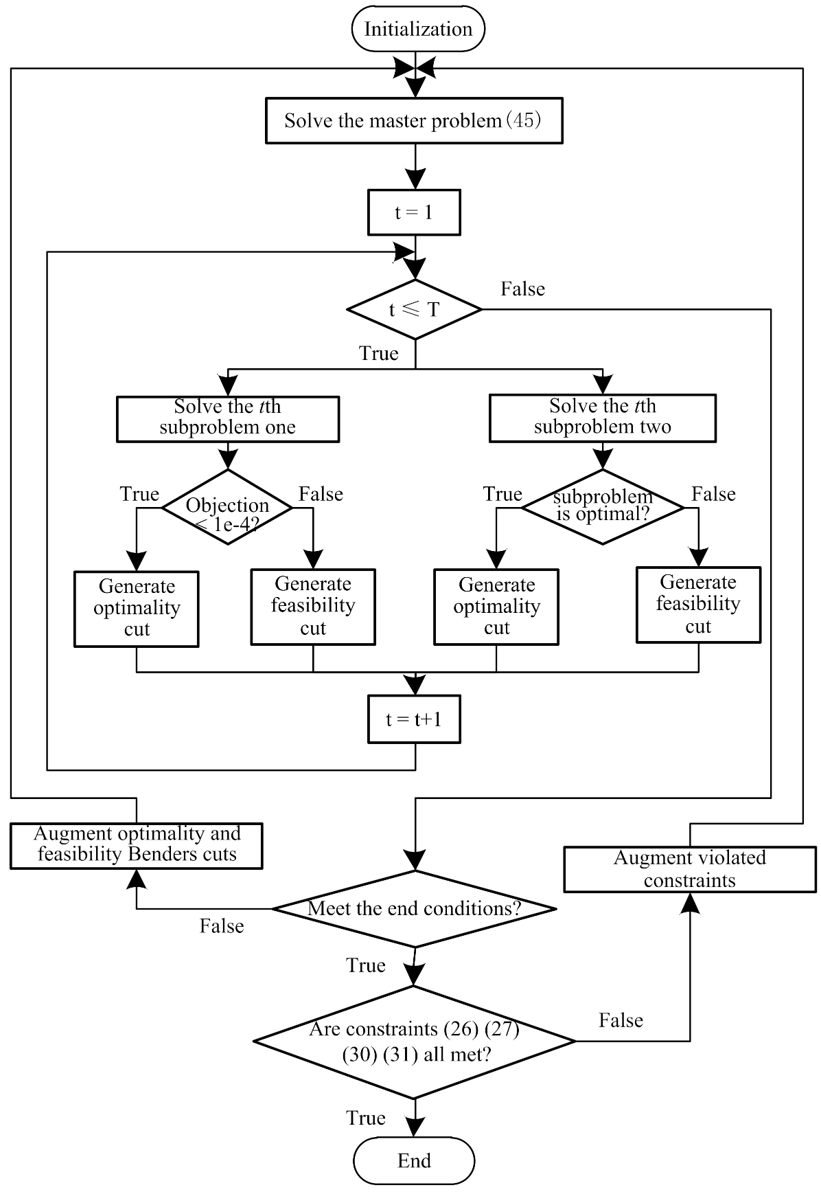
• The algorithm parameters are initialized, the number of iterations is set to zero, the upper bound (UB) and the lower bound (LB) are set to positive and negative infinity, respectively;
• The main problem (45) is solved with the sum of substitution variables being zero and benders optimal cut set and feasible cut set being empty, and the results of generator start-up, stop, active power and rotating reserve power, energy storage charging and discharging state and charging and discharging power, and wind power photovoltaic active power output are obtained;
• The first sub-problem is solved with the data stream obtained from the main problem. If the optimization result is feasible, benders optimal cut is generated according to Equation (47); if the optimization result is not feasible, benders feasibility cut is generated according to Equation (48);
• The second sub-problem is solved by the data stream obtained from the main problem. If the optimization result is not feasible, benders feasibility cut is generated according to the formula; if the optimization result is feasible, benders optimal cut is generated according to the formula;
• If all the first and second sub-problems in the scheduling cycle are feasible, then go to the next step, otherwise go to the seventh step;
• Calculate the value of the dual gap and judge whether it meets the threshold of the end of the algorithm iteration. If it meets, go to step 8. If not, go to the next step;
• Add the optimal cut set and feasible cut set to the main problem to get the new data stream and, then, go to the third step.
• Calculate whether the network security constraints satisfy the constraints (26), (27), (30), and (31) in N and N-1 states. If all the constraints are satisfied, the optimization results are output and the algorithm ends. Otherwise, the unsatisfied constraints are added to the main problem, and the second step is to solve it again.

4. Numerical Case Studies

In order to verify the correctness and feasibility of the above model and algorithm, IEEE RTS-24 system [37] is selected for test. The total installed capacity of this system is 3405 MW. All thermal generator parameters contained in the test system are shown in

Table 1. Summary of all thermal power units contained in the test system.

Unit	Node	Technology	${\mathit{P}}_{\mathit{i}}^{\max }$ (MW)	${\mathit{P}}_{\mathit{i}}^{\min }$ (MW)	${\mathit{P}}_{\mathit{i}}^{\mathrm{up}}$ (MW/h)	${\mathit{P}}_{\mathit{i}}^{\mathrm{down}}$ (MW/h)	UT (h)	DT (h)	Noload Costs (USD)	${\mathit{c}}_{\mathit{i}}^1$ (USD/MW)	${\mathit{c}}_{\mathit{i}}^2$ (USD/MW)	${\mathit{c}}_{\mathit{i}}^3$ (USD/MW)
1–2	1	OCGT	20	8	90	100	2	1	454.6	28.97	29.24	29.70
3–4	1	CCGT	76	40	120	120	3	2	263.4	18.42	19.23	20.11
5–6	2	OCGT	20	8	90	100	2	1	454.6	28.97	29.24	29.70
7–8	2	CCGT	76	40	120	120	3	2	263.4	18.42	19.23	20.11
9–11	7	CCGT	100	10	420	420	4	2	306.6	17.59	18.28	18.96
12–14	13	CCGT	197	104	310	310	4	3	482.9	17.21	17.71	18.23
15–19	15	OCGT	12	5.4	60	70	2	1	365.5	29.46	30.13	30.86
20	15	IGCC	155	54.24	70	80	24	16	415.5	23.81	24.52	25.25
21	16	IGCC	155	54.24	70	80	24	16	415.5	23.81	24.52	25.25
22	18	Nuclear	400	100	280	280	168	24	188.3	6.96	7.23	7.50
23	21	Nuclear	400	100	280	280	168	24	188.3	6.96	7.23	7.50
24–29	22	CCGT	50	26	120	120	2	1	626.1	28.31	29.25	30.49
30–31	23	IGCC	155	54.24	70	80	24	16	415.5	23.81	24.52	25.25
32	23	Coal	350	140	140	140	8	5	303.8	26.21	26.71	27.20

. In addition, six wind farms with a capacity of 260 MW are connected to buses 2, 3, 5, 8, 17, and 21 of the system, three photovoltaic power stations with capacity of 400 MW are connected to buses 6, 16, and 23, and six sodium flow battery energy storage power stations with rated capacity of 100 MW are connected to buses 1, 2, 3, 5, 6, and 10. See Figure 2 for the schematic diagram of the grid placement of the power units. Nuclear power units participate in peak load regulation operation of power grid according to G mode “15-1-7-1” and maximum 50% [38]. The peak time electricity price of the system is 125 USD/MWh; the average electricity price is 78 USD/MWh; the valley time tariff is 31 USD/MWh; the energy storage conversion efficiency is 80%, and the complete charge/discharge time is 8 h; the penalty cost of wind/photovoltaic is 40 USD/MWh; let mean interval conservative coefficient be equal to variance interval conservative coefficient; the confidence level of each robust chance constraint is equal. Julia0.6 is selected as the programming language, CPLEX12.7 is used as the main problem solver, and Ipopt3.1 is used to solve the nonlinear AC sub-problems. All the calculations are completed on a computer equipped with Intel Core i5-2310 2.9GHz.

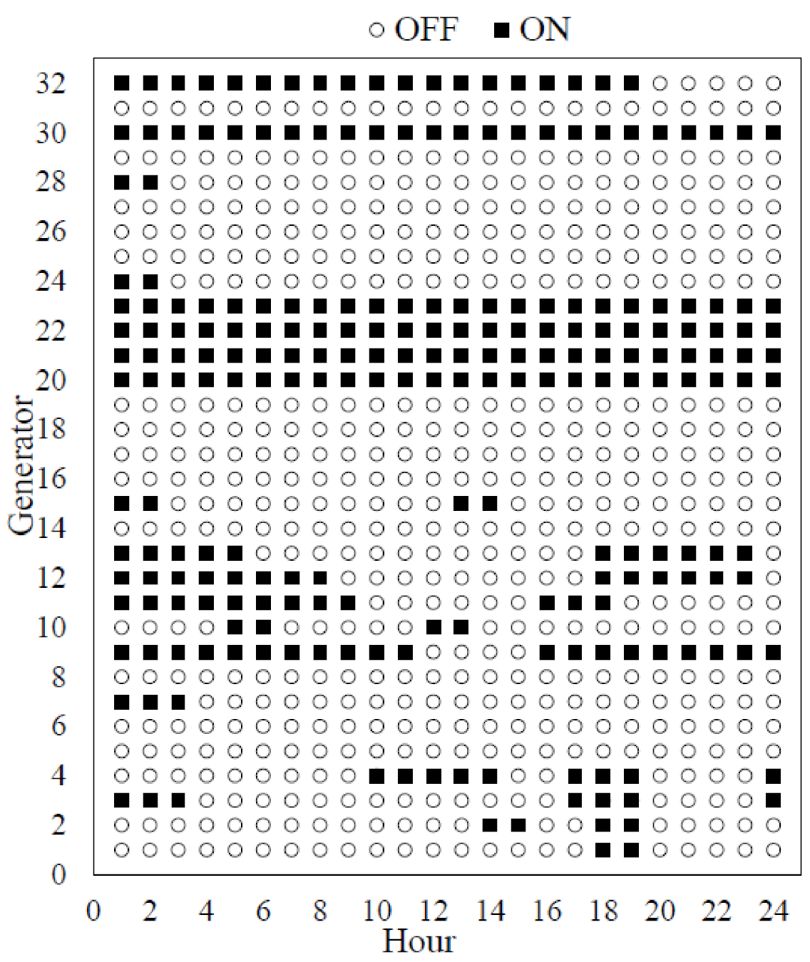
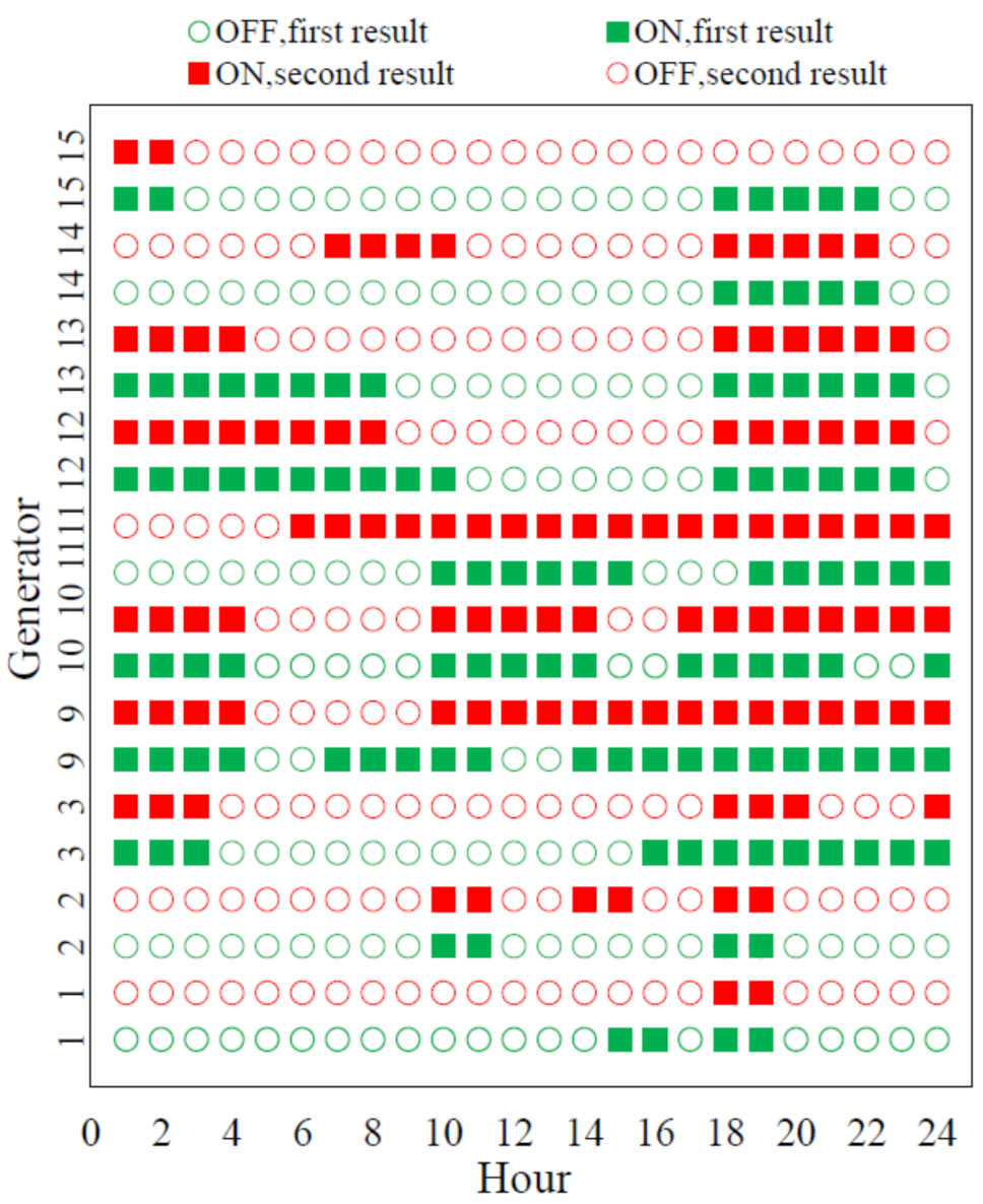
4.1. The Results of This Model

Using this method to simulate the test system, the confidence level is 0.992, and the conservative coefficient is 0.6. The results of the next day 24-hour conventional unit start-up and shutdown are shown in Figure 3. It is easy to see that two nuclear power units, 22 and 23, and three large capacity thermal power units, 20, 21, and 30, start-up at all times to provide extra base load. Other thermal power units with smaller capacity start and stop according to the changes in load and wind and photovoltaic power output.

The hourly online generator capacity (OGC), wind, and photovoltaic power output, energy storage charge and discharge power, and spinning reserve power are shown in Figure 4. It can be seen that the energy storage charge is concentrated in the valley period, and the energy storage discharge is concentrated in the peak period, indicating the feasibility of the decision results. Furthermore, by changing the parameters of the model, sensitivity analysis was used to detect the influence of the parameters on the UC results.

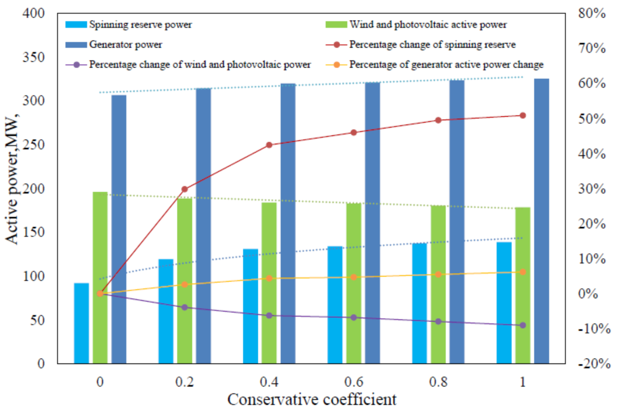
4.2. Influence of Conservative Coefficient on Objection

The fixed confidence level is 0.99. When the conservative coefficient changes from 0.001 to 1.0, the change details of the total generation cost of the test system are shown in

Table 2. Object value of different conservative coefficients.

${\mathbf{\Gamma }}_{\mathit{\sigma }},{\mathbf{\Gamma }}_{\mathit{\mu }}$	Power Flow	Reserve Cost/USD	Penalty Cost/USD	Fuel Cost/USD	Objection/USD
0.001	AC	91,968	13,595	572,691	627,738
0.2		119,377	44,340	593,714	710,645
0.4		130,961	62,423	623,802	767,520
0.6		134,236	66,844	629,503	780,846
0.8		137,466	75,979	638,049	802,159
1		138,750	84,398	640,529	814,397
0	DC	91,968	13,223	568,113	625,064
0.2		119,377	43,340	592,763	708,703
0.4		130,961	59,610	620,243	760,830
0.6		134,236	63,431	626,464	774,388
0.8		137,466	73,222	633,233	798,928
1		138,750	80,420	639,155	809,511

. In order to compare the influence of AC and DC power flow on UC results, the table also gives the UC optimization results based on DC.

It can be seen from the Table 2 that with the gradual increase in the conservative coefficient, the spinning reserve cost, the penalty cost, and the total power generation cost of the system gradually increase, resulting in the gradual increase in the objection value. The change trend of them with the conservative coefficient is shown in Figure 5. It can be seen that when the conservative coefficient increases from 0.001 to 1, the spinning reserve power increases significantly synchronously, with a cumulative increase of 50%; the active power of the generator increases slowly with a cumulative increase of 6%; the active power output of wind and photovoltaic decreased slowly with the increase in conservative coefficient, with a cumulative decrease of 9%. The reduction in wind and photovoltaic power output indicates that the proportion of wind and photovoltaic energy consumption is reduced, and the abandoned wind and photovoltaic power is increased. The reason is that the increase in the conservative coefficient means that the fluctuation range of the forecast error becomes larger, which indicates that the accuracy of the wind and photovoltaic power output forecast decreases. At this time, in order to cope with the uncertainty of the continuous increase in wind and photovoltaic power and meet the safety requirements of power system operation as far as possible, more spinning reserve capacity is bound to be reserved, which leads to the increase in the generation cost of conventional units. In addition, the accuracy of wind and photovoltaic output forecast is reduced, which will increase the power of abandoned wind and solar power and, then, increase the cost of abandoned wind and solar power. These two reasons lead to the increase in the objection value.

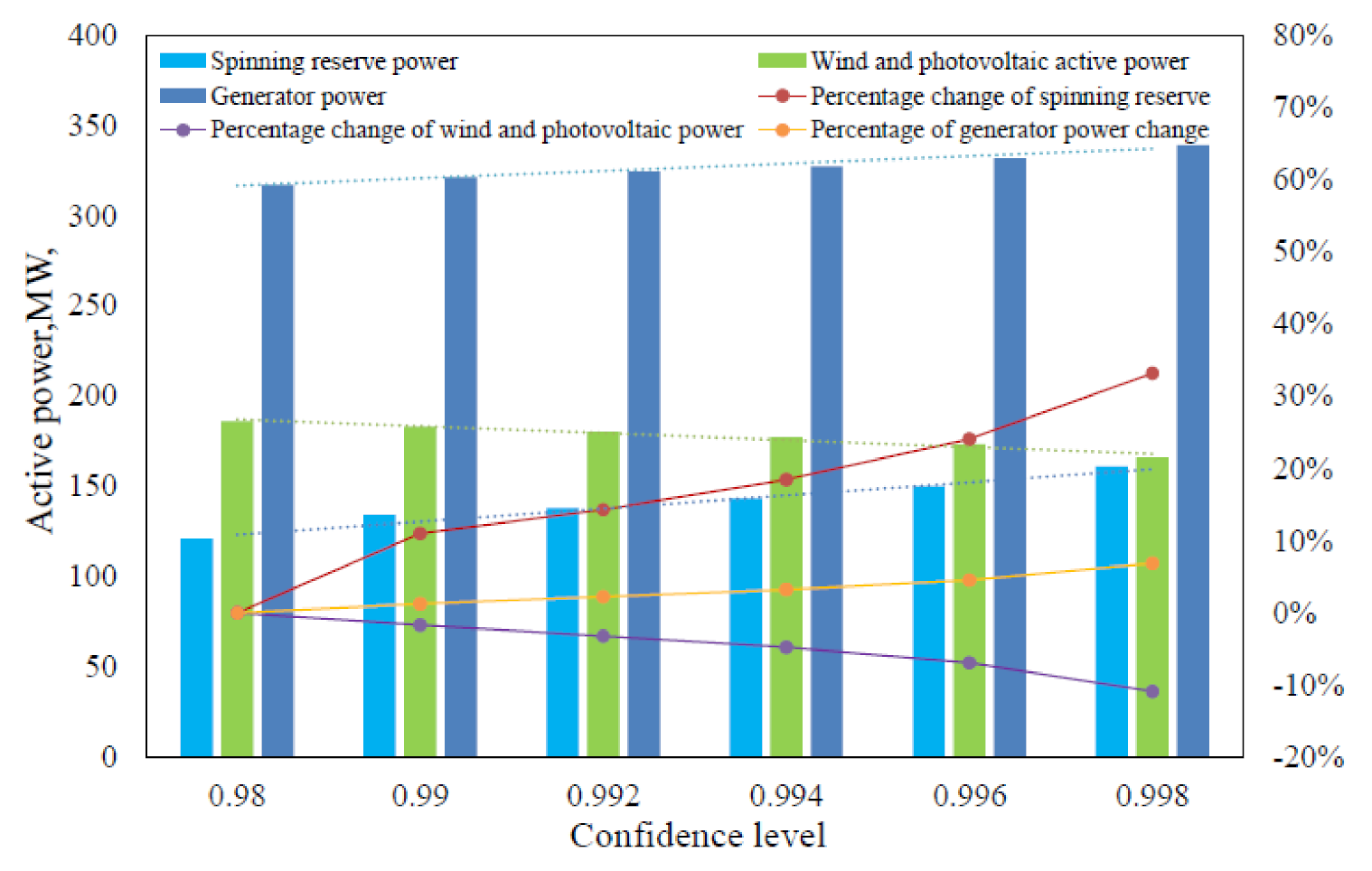
4.3. Influence of Confidence Level on Objection

The change in the objection value when the confidence level changes from 0.98 to 0.998 is shown in

Table 3. Object value of different confidence levels.

${\mathit{\epsilon }}_{\mathit{i}}^{\mathrm{G}},{\mathit{\epsilon }}_{\mathit{l}}^{\mathrm{L}}$	Power Flow	Reserve COST/USD	Penalty Cost/USD	Fuel Cost/USD	Objection/USD
0.02	AC	120,974	54,096	599,869	723,844
0.01		134,236	66,844	629,503	780,846
0.008		138,253	78,032	634,329	802,046
0.006		143,275	89,658	642,196	826,545
0.004		150,083	105,532	657,015	865,024
0.002		161,082	135,132	677,079	929,561
0.02	DC	120,974	48,721	598,148	720,156
0.01		134,236	63,431	626,464	774,388
0.008		138,253	74,450	630,581	794,805
0.006		143,275	87,215	640,130	822,573
0.004		150,083	105,532	657,015	865,024
0.002		161,082	135,132	677,079	929,561

. As a comparison, the optimization results considering only DC power flow are given.

It can be seen from Table 3 that with the gradual increase in the confidence level, the spinning reserve cost, abandonment cost, and fuel cost of the system gradually increase, resulting in the gradual increase in the objection value. The change trend of them with the confidence level is shown in Figure 6. It can be seen that when the confidence level gradually increases from 0.98 to 0.998, the synchronous increase in spinning reserve is obvious, and the cumulative increase is 33%; the active power of the generator increases slowly with a cumulative increase of 7%; the output power of wind and photovoltaic decreased slowly with the increase in conservative coefficient, with a cumulative decrease of 10%. The increase in confidence level means the increase in risk level of generator output and line power flow out of limit. When the chance constraint meets higher constraint probability, its corresponding feasible region is narrowed, and the optimization in the smaller feasible region must be at the expense of certain economic objection value.

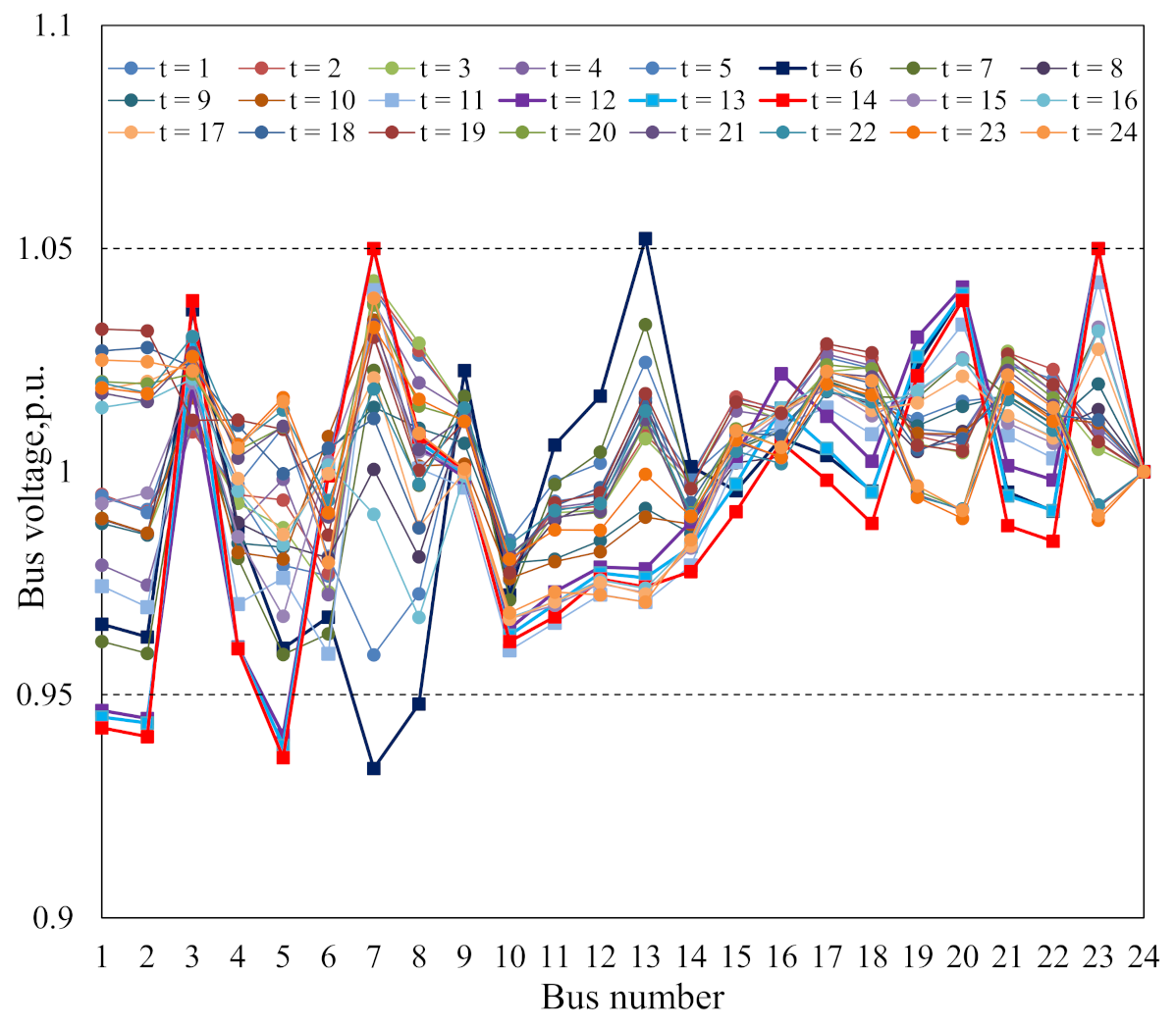
4.4. Influence of AC Power Flow on Optimization Results

Compared with the optimization results without considering AC power flow in Table 2 and Table 3, when the parameters are consistent, the UC objection value, fuel cost, and abandoned wind and solar energy cost increase slightly with considering AC power flow, and the target value in Table 2 increases by 0.27–0.88%; the increase in fuel cost is between 0.16% and 0.81%, and the increase in abandoned wind and solar energy cost is between 2.3% and 5.4%. In Table 3, the objection value increases between 0% and 0.9%; the increase in fuel cost is between 0% and 0.59%, and the increase in abandoned wind and solar energy cost is between 0% and 11%.

The UC model based on DC does not consider the influence of reactive power and node voltage on the optimization results, which may lead to reactive power imbalance, and then, cause the risk of under voltage or over voltage on some buses. From the optimization results in Table 2 and Table 3, it can be seen that only when the confidence level is greater than or equal to 0.996, the optimization results meet the reactive power balance. All bus node voltages are within the allowable fluctuation range. In order to investigate the influence of AC on start-up, shutdown, and node voltage in detail, the conservative coefficient of 0.6 and confidence level of 0.992 are selected to optimize the calculation and track the iterative process. The results of the first solution of the main problem are substituted into the AC check sub-problem, and all bus node voltages are shown in Figure 7.

It is easy to see that there are three times of node voltage overrun in the sixth period, in which the lower limit of bus 7 is 1.74%, the lower limit of bus 8 is 0.22%, and the higher limit of bus 13 is 0.21%. In the 12th period, there were three instances of node voltage overrun, in which the lower limit of bus 1 was 0.37%, the lower limit of bus 2 was 0.56%, and the lower limit of bus 5 was 0.95%. In the 13th period, there were three instances of node voltage overrun, in which the lower limit of bus 1 was 0.53%, the lower limit of bus 2 was 0.67%, and the lower limit of bus 5 was 1.2%. In the 14th period, there were three instances of node voltage overrun, in which the lower limit of bus 1 was 0.78%, the lower limit of bus 2 was 0.99%, and the lower limit of bus 5 was 1.5%. It is easy to see that most of the voltage overruns are that the node voltage is less than the minimum limit, and the maximum overrun of 1.74% occurs at bus 7 of period 6. Usually, the node voltage is too low because of the lack of reactive power supply, which indicates that it is necessary to increase the number of generators started in these periods when the AC power flow is not feasible to increase the reactive power supply. According to the generated benders cut, it is returned to the main problem for the second solution. The comparison of unit startup and shutdown obtained from the two main problems is shown in Figure 8.

Through the comparison, it can be found that the main changes are in six periods, 11 units are added, nine units are added in 12 and 13 periods, and two units are added in 14 periods. Because these units are added with reactive power, the voltage of out-of-limit node returns to the limit range. Finally, after 14 iterations, the voltage of all nodes in the whole scheduling cycle is within the limit. It can be seen that UC considering AC power flow constraints can comprehensively consider the impact of reactive power and node voltage on system power generation capacity and line power flow when making a unit start-up and shutdown plan and ensure node voltage safety by coordinating and adjusting the unit start-up and shutdown status and output in advance.

4.5. Comparison with Stochastic Unit Commitment Model

In order to investigate the feasibility and calculation efficiency of the proposed model, the chance-constrained unit commitment [39] is selected and compared with the proposed model. In order to make the comparison more real and effective, the AC verification sub-problem is added to the CCUC model. The calculation objection value of the model is shown in Figure 9. It can be seen from the figure that the conservative coefficient is infinitely close to 0 regardless of the confidence level. It means that the fluctuation range of mean and variance is infinitesimal and close to 0. At this time, the mean and variance are close to a fixed value. The model in this paper is similar to the traditional chance-constrained model. From the calculation results of the two models, it can be seen that the results calculated by this method are very close to the results obtained by traditional chance-constrained SOC transformation, and the error is between 0.027% and 0.58%. It is shown that the proposed cut algorithm has high accuracy.

The iteration and calculation time of the main and subproblem of the model in this paper are shown in

Table 4. Algorithm calculation efficiency comparison.

${\mathit{\epsilon }}_{\mathit{i}}^{\mathrm{G}},{\mathit{\epsilon }}_{\mathit{l}}^{\mathrm{L}}$	Algorithm	Iterations	Master Problem/s	Subproblem/s	Total/s
0.02	DRSCUC	7	120	20	980
0.01		5	135	20	775
0.008		4	150	20	680
0.006		6	165	20	1110
0.004		5	180	20	1000
0.002		5	210	20	1150
0.02	CCSCUC	5	300	20	1600
0.01		3	330	20	1050
0.008		2	380	20	800
0.006		4	440	20	1840
0.004		3	520	20	1620
0.002		4	600	20	2480

.The results show that under different confidence levels, the number of iterations of the main sub-problem is slightly larger than that of the CCUC, and the solving time of the sub-problem is consistent with that of CCUC, but the total computing time is significantly lower than that of CCUC, After analysis, it is considered that this is mainly because the cutting plane algorithm proposed for distributed robust chance constraints greatly reduces the complexity of the main problem model and the solution time of the main problem. Furthermore, it shows that this algorithm has high computational efficiency and can meet the requirements of the actual system.

5. Conclusions

In order to solve the problem of insufficient historical data and unknown real probability distribution of wind and photovoltaic power output, this paper improves the traditional chance-constrained unit commitment model. Firstly, the general moment uncertainty distribution set of wind and photovoltaic power forecast error is selected, its polyhedral expression is given, and an improved cut plane algorithm is proposed; secondly, the AC power flow model, which truly reflects the physical law of power grid operation, is adopted to ensure the node voltage security and improve the accuracy of UC results. Through comparative analysis of simulation examples, the following conclusions are obtained.

(1) In this model, the uncertainty of renewable energy output of UC is transformed into a conservative coefficient, and the risk of generator output and line power flow out of limit is transformed into the confidence level. After selecting reasonable conservative coefficient and confidence level, the UC optimization results of this model can achieve the decision goal of minimizing operation cost under certain risk.

(2) Under the premise that the objection value of UC based on AC is less than 1.0%, the safety margin of bus voltage is significantly improved, and the risk of bus voltage overrun is reduced, so as to improve the safety of system operation.

(3) The simulation results show that the larger the range of uncertainty set, the greater the total scheduling cost of the system. Under different confidence levels, the optimal scheduling results focusing on economy or security are different. Compared with the chance-constrained method with specific distribution, the results show that the moment uncertain distribution robust optimization method has good computational accuracy and higher computational efficiency.

References

1. Xia, Q.; Zhong, H.; Kang, C. Review and Prospects of the Security Constrained Unit Commitment Theory and Applications. Proc. CSEE 2013, 33, 94–103. [Google Scholar]
2. Zhao, C.; Guan, Y. Data-Driven Stochastic Unit Commitment for Integrating Wind Generation. IEEE Trans. Power Syst. 2015, 31, 2587–2596. [Google Scholar] [CrossRef]
3. Uckun, C.; Botterud, A.; Birge, J. An Improved Stochastic Unit Commitment Formulation to Accommodate Wind Uncertainty. IEEE Trans. Power Syst. 2015, 31, 2507–2517. [Google Scholar] [CrossRef]
4. Wang, C.; Wei, H.; Wu, S. Stochastic-Security-Constrained Unit Commitment Considering Uncertainty of Wind Power. Power Syst. Technol. 2017, 41, 1419–1427. [Google Scholar]
5. Wang, B.; Wang, S.; Zhou, X.; Watada, J. Multi-objective unit commitment with wind penetration and emission concerns under stochastic and fuzzy uncertainties. Energy 2016, 111, 18–31. [Google Scholar] [CrossRef]
6. Wu, Z.; Zeng, P.; Zhang, X.-P.; Zhou, Q. A Solution to the Chance-Constrained Two-Stage Stochastic Program for Unit Commitment With Wind Energy Integration. IEEE Trans. Power Syst. 2016, 31, 4185–4196. [Google Scholar] [CrossRef]
7. Bertsimas, D.; Litvinov, E.; Sun, X.A.; Zhao, J.; Zheng, T. Adaptive Robust Optimization for the Security Constrained Unit Commitment Problem. IEEE Trans. Power Syst. 2013, 28, 52–63. [Google Scholar] [CrossRef]
8. Wu, W.; Wang, K.; Li, G. Affinely Adjustable Robust Unit Commitment Considering the Spatiotemporal Correlation of Wind Power. Proc. CSEE 2017, 37, 4089–4097. [Google Scholar]
9. Xiong, P.; Jirutitijaroen, P. Two-stage adjustable robust optimization for unit commitment under uncertainty. IET Gener. Transm. Distrib. 2014, 8, 573–582. [Google Scholar] [CrossRef]
10. Fan, L.; Wang, K.; Li, G.; Wu, W.; Ge, W. Robust Unit Commitment Considering Temporal Correlation of Wind Power. Autom. Electr. Power Syst. 2018, 42, 91–97. [Google Scholar]
11. Xiong, P.; Jirutitijaroen, P.; Singh, C. A Distributionally Robust Optimization Model for Unit Commitment Considering Uncertain Wind Power Generation. IEEE Trans. Power Syst. 2017, 32, 39–49. [Google Scholar] [CrossRef]
12. Zhao, C.; Jiang, R. Distributionally Robust Contingency-Constrained Unit Commitment. IEEE Trans. Power Syst. 2017, 33, 94–102. [Google Scholar] [CrossRef]
13. Wang, Z.; Bian, Q.; Xin, H.; Gan, D. A distributionally robust co-ordinated reserve scheduling model considering CVaR-based wind power reserve requirements. IEEE Trans. Sustain. Energy 2016, 7, 625–636. [Google Scholar] [CrossRef]
14. Xie, W.; Ahmed, S. Distributionally robust chance constrained optimal power flow with renewables: A conic reformulation. IEEE Trans. Power Syst. 2018, 33, 1860–1867. [Google Scholar] [CrossRef]
15. Zhang, Y.; Wang, J.; Ding, T.; Wang, X. Conditional value at risk-based stochastic unit commitment considering the uncertainty of wind power generation. IET Gener. Transm. Distrib. 2018, 12, 482–489. [Google Scholar] [CrossRef]
16. Xiong, P.; Singh, C. Optimal Planning of Storage in Power Systems Integrated with Wind Power Generation. IEEE Trans. Sustain. Energy 2015, 7, 232–240. [Google Scholar] [CrossRef]
17. Yang, Y.; Lei, X.; Zhai, Q.; Wu, J.; Guan, X. Transmission capacity margin assessment in power systems with uncertain wind integration. In Proceedings of the 2017 13th IEEE Conference on Automation Science and Engineering (CASE), Xi’an, China, 20–23 August 2017. [Google Scholar]
18. Tarnowski, G.C.; Kjær, P.C.; Dalsgaard, S.; Nyborg, A. Regulation and frequency response service capability of modern wind power plants. In Proceedings of the IEEE Power & Energy Society General Meeting, Minneapolis, MN, USA, 25–29 July 2010. [Google Scholar]
19. Lin, Y.; Yang, M.; Wan, C.; Wang, J.; Song, Y. A Multi-Model Combination Approach for Probabilistic Wind Power Forecasting. IEEE Trans. Sustain. Energy 2019, 10, 226–237. [Google Scholar] [CrossRef]
20. Luig, A.; Bofinger, S.; Beyer, H.G. Analysis of confidence intervals for the prediction of regional wind power out-put. In Proceedings of the European Wind Energy Association Conference, Copenhagen, Denmark, 1 January 2001; pp. 725–728. [Google Scholar]
21. Tewari, S.; Geyer, C.J.; Mohan, N. A Statistical Model for Wind Power Forecast Error and its Application to the Estimation of Penalties in Liberalized Markets. IEEE Trans. Power Syst. 2011, 26, 2031–2039. [Google Scholar] [CrossRef]
22. Hodge, B.; Milligan, M. Wind power forecasting error distributions over multiple time scales. In Proceedings of the Power and Energy Society General Meeting, Detroit, MI, USA, 24–29 July 2011. [Google Scholar]
23. Bruninx, K.; Delarue, E. A Statistical Description of the Error on Wind Power Forecasts for Probabilistic Reserve Sizing. IEEE Trans. Sustain. Energy 2014, 5, 995–1002. [Google Scholar] [CrossRef]
24. Liu, M.; Zeng, C.; Miao, H. Unit commitment model based on distributionally robust chance constraints. Electr. Meas. & Instrum. 2021, 58, 32–36. [Google Scholar] [CrossRef]
25. Shi, Y.; Wang, L.; Chen, W.; Guo, C. Distributed Robust Unit Commitment with Energy Storage Based on Forecasting Error Clusting of Wind Power. Autom. Electr. Power Syst. 2019, 43, 3–12. [Google Scholar] [CrossRef]
26. Wei, W.; Liu, F.; Mei, S. Distributionally Robust Co-Optimization of Energy and Reserve Dispatch. IEEE Trans. Sustain. Energy 2015, 7, 289–300. [Google Scholar] [CrossRef]
27. Zhang, Y.; Shen, S.; Mathieu, J.L. Distributionally robust chance-constrained optimal power flow with uncertain renewables and uncertain reserves provided by loads. IEEE Trans. Power Systems 2017, 32, 1378–1388. [Google Scholar] [CrossRef]
28. Liu, S.; Jian, J.; Wang, Y.; Liang, J. A robust optimization approach to wind farm diversification. Int. J. Electr. Power Energy Syst. 2013, 53, 409–415. [Google Scholar] [CrossRef]
29. Wang, S.; Li, B.; Yu, J.; Xu, T. Analysis on Time-Varying Characteristics of Probability Error in Forecast of Wind Speed and Wind Power. Power Syst. Technol. 2013, 37, 967–973. [Google Scholar]
30. Xie, L.; Gu, Y.; Zhu, X.; Genton, M.G. Short-Term Spatio-Temporal Wind Power Forecast in Robust Look-ahead Power System Dispatch. IEEE Trans. Smart Grid 2014, 5, 511–520. [Google Scholar] [CrossRef]
31. Delage, E.; Ye, Y. Distributionally robust optimization under moment uncertainty with application to data-driven problems. Oper. Res. 2010, 58, 595–612. [Google Scholar] [CrossRef] [Green Version]
32. Cheng, J.; Lisser, A.; Letournel, M. Distributionally robust stochastic shortest path problem. Electron. Notes Discret. Math. 2013, 41, 511–518. [Google Scholar] [CrossRef]
33. Benders, J.F. Partitioning procedures for solving mixed-variables programming problems. Numer. Math. 1962, 4, 238–252. [Google Scholar] [CrossRef]
34. Sha, Q.; Wang, W. Optimal Allocation of Energy Storage Considering N-1 Security Constraints Based on Chance Constraints. Adv. Eng. Sci. 2019, 51, 147–156. [Google Scholar]
35. Lubin, M.; Dvorkin, Y.; Backhaus, S. A Robust Approach to Chance Constrained Optimal Power Flow with Renewable Generation. IEEE Trans. Power Syst. 2015, 31, 3840–3849. [Google Scholar] [CrossRef] [Green Version]
36. Wang, C.; Wei, H.; Wu, S. A Decomposition coordination Algorithm Applied to Hydro-thermal Unit Commitment Problems With Power Flow Constraints. Proc. CSEE 2017, 37, 3148–3161. [Google Scholar]
37. Grigg, C.; Wong, P.; Albrecht, P.; Allan, R.; Bhavaraju, M.; Billinton, R.; Chen, Q.; Fong, C.; Haddad, S.; Kuruganty, S.; et al. The IEEE Reliability Test System-1996. A report prepared by the Reliability Test System Task Force of the Application of Probability Methods Subcommittee. IEEE Trans. Power Syst. 1999, 14, 1010–1020. [Google Scholar] [CrossRef]
38. Zhao, J.; Liu, D.; Lei, Q.; Du, Z.; Wang, J.; Zhou, L.; Huang, Y. Analysis of nuclear power plant participating in peak load regulation of power grid and combined operation with pumped storage power plant. Proc. CSEE 2011, 31, 1–6. [Google Scholar]
39. Wang, B.; Yang, X.; Short, T.; Yang, S. Chance constrained unit commitment considering comprehensive modelling of demand response resources. IET Renew. Power Gener. 2017, 11, 490–500. [Google Scholar] [CrossRef]
Figure 1. Flow chart of the proposed algorithm.
Energies 14 05618 g001
Figure 2. Schematic diagram of the grid.
Energies 14 05618 g002
Figure 3. On and off status of thermal power units.
Energies 14 05618 g003
Figure 4. Status of source and load and storage.
Energies 14 05618 g004
Figure 5. Variation of generator and wind power with different conservative coefficient.
Energies 14 05618 g005
Figure 6. Variation of generator and wind power with different confidence level.
Energies 14 05618 g006
Figure 7. First iteration bus voltage.
Energies 14 05618 g007
Figure 8. On and off status of generator.
Energies 14 05618 g008
Figure 9. Comparison of model calculation results.
Energies 14 05618 g009