Article

Optimization Algorithms: Optimal Parameters Computation for Modeling the Polarization Curves of a PEFC Considering the Effect of the Relative Humidity

by
Ángel Encalada-Dávila
,
Samir Echeverría
,
Jordy Santana-Villamar
,
Gabriel Cedeño
and
Mayken Espinoza-Andaluz
*,†
Escuela Superior Politécnica del Litoral (ESPOL), Facultad de Ingeniería Mecánica y Ciencias de la Producción, Centro de Energías Renovables y Alternativas, Campus Gustavo Galindo Km. 30.5 Vía Perimetral, Guayaquil P.O. Box 09-01-5863, Ecuador
*
Author to whom correspondence should be addressed.
These authors contributed equally to this work.
Energies 2021, 14(18), 5631; https://doi.org/10.3390/en14185631
Submission received: 9 August 2021 / Accepted: 25 August 2021 / Published: 7 September 2021
(This article belongs to the Special Issue Design, Modeling, and Optimization of Novel Fuel Cell Systems)

Abstract

:
The development of green energy conversion devices has been promising to face climate change and global warming challenges over the last few years. Energy applications require a confident performance prediction, especially in polymer electrolyte fuel cell (PEFC), to guarantee optimal operation. Several researchers have employed optimization algorithms (OAs) to identify operating parameters to improve the PEFC performance. In the current study, several nature-based OAs have been performed to compute the optimal parameters used to describe the polarization curves in a PEFC. Different relative humidity (RH) values, one of the most influential variables on PEFC performance, have been considered. To develop this study, experimental data have been collected from a lab-scale fuel cell test system establishing different RH percentages, from 18 to 100%. OAs like neural network algorithm (NNA), improved grey-wolf optimizer (I-GWO), ant lion optimizer (ALO), bird swarm algorithm (BSA), and multi-verse optimization (MVO) were evaluated and compared using statistical parameters as training error and time. Results gave enough information to conclude that NNA had better performance and showed better results over other highlighted OAs. Finally, it was found that sparsity and noise are more present at lower relative humidity values. At low RH, a PEFC operates under critical conditions, affecting the fitting on OAs.

1. Introduction

In the last few years, several studies related to renewable energy technologies have been performed [1,2,3,4]. The development of new energy sources with high efficiency and environmentally friendliness is one of the challenges of today’s world. The fossil fuels currently used are unsustainable and have considerable impacts on the environment. The mentioned fossil fuels are the primary source to produce the consumed energy, causing severe environmental problems like climate change and pollution. In 2005, they were estimated to produce 80% of the world’s primary energy [5]. In the same year, 16.5% of the world’s primary energy was produced by renewable energy and expected to replace 80% of fossil fuels up to 2050, i.e., in about four decades [6]. This aim is in line with the European Green Deal proposed in 2011 [7].
Polymer electrolyte fuel cells (PEFCs) are presented as one of the applications of hydrogen technology that can be used to meet energy requirements. PEFCs are electrochemical devices that transform the energy from chemical reactions into electrical energy [8]. The energy conversion is done in a single process compared to combustion engines engines, in which the energy conversion is performed in multiple steps [9]. Furthermore, the energy conversion process in a PEFC is based on three main stages: hydrogen as the fuel flow at the anode while oxygen as oxidant flows through the cathode, the gas molecules are split at the active region of the membrane electrode assembly (MEA), and, finally, free electrons are transported out to the cell producing clean electrical energy. Apart from this, it can categorized in different types [10,11]. PEFCs are one of the most promising energy conversion devices to produce electricity with zero emission. In addition, it can work at low pressure, low temperature, noiseless manner, and at different current densities with high efficiency [8].
To study the behavior of a PEFC, polarization curves are typically used. The different parameters that affect their performance like temperature, relative humidity (RH), pressure, oxidant/fuel flow, and dry conditions are usually varied [12,13,14]. The polarization curves present the voltage as a function of the current density. In the mentioned curves, three regions are clearly distinguished: activation, ohmic, and concentration region. The activation region represents the energy required to start reactions at low current densities. On the other hand, the ohmic region occurs at moderate current densities and represents the ohmic losses inside the PEFC. Finally, the region of concentration losses occurs due to the abundant generation of liquid water blocking the pores of the diffusion media (DM) at high-density currents, and this impairs the development of electrochemical reactions [15].
To accomplish the optimum operation of PEFCs, several studies have been dealing with the problem of accurately identifying its internal electrochemical and mechanical parameters by modeling and simulation [16,17]. The modeling procedures may be classified as mechanical or experimental modeling. Mechanical modeling deals with the electrochemical, heat, and mass transport parameters. The experimental modeling is performed partially from the mechanical one and formulated as empirical equations [18,19,20,21,22].
The models of PEFCs should be viable, computationally effective, and capable of predicting their performances over a wide range of operating environmental conditions [23]. Appropriate model identifications can be ensured by entering correct input parameters in the governing equations of the PEFC, which comprise chemical and physical properties. The modeling methodologies of PEFCs can either be theoretical, semi-empirical, or empirical [24,25,26].
Over the last few decades, there has been a variety of studies related to PEFCs parameters’ identifications using heuristic-based methods, such as particle swarm optimization (PSO) [27], which is used to define the parameters of steady-state PEFC models. In addition, an improved grey-wolf optimizer algorithm (I-GWO) and multiverse optimization (MVO) algorithm have been applied to accomplish the same goal. The ant–lion optimizer (ALO) algorithm has also been implemented to model PEFCs [28].
Correctly identifying the unspecified parameters leads to the actual model of a PEFC. Previous studies related to determining the optimal parameters of FCs are described as follows. For example, Priya et al. [29] utilized a simple genetic algorithm to obtain the accurate model of a PEFC by identifying the optimal parameters and used the derivative of power with respect to current as the objective function (OF). Gong et al. [30] applied a differential evolution method to obtain the optimal parameters of a PEFC. This algorithm can also include a ranking-based operator to accelerate the convergence of the solutions. On the other hand, Ye et al. [31] used PSO to identify PEFC parameters to minimize its OF, which was based on the calculated and measured stack voltage. Likewise, Fathy et al. [32] introduced an MVO methodology to determine the optimal parameters of a PEFC. Ali et al. [33] applied I-GWO to successfully identify the unknown parameters of five types of commercial PEFCs.
Applying optimization algorithms (OAs) to the PEFC performance gives excellent results, which will allow the researchers to obtain the representative equation of a PEFC model successfully. The main idea behind this is that they can escape from the local minimum, which leads them to obtaining almost the global optimum [34]. Taking into consideration the mentioned methods and their promising results in generating high-quality solutions, these meta-heuristic processes have been widely used to model PEFCs, so there is much potential for improvement in this area [35].
A few applications of heuristic-based methods to define models of PEFCs are addressed. However, due to the high nonlinearity of PEFC models, the extraction of optimal values of parameters is crucial, which means that small deviations of these values may dramatically affect the quality of such models [23]. Therefore, the nonlinear behavior of the models motivates the researchers to develop and use improved algorithms like I-GWO to define the parameters of a PEFC. According to the aforementioned, OA can deal efficiently with uni and multi-modal engineering optimization problems [36].
This paper focuses the study on the computation of the optimal parameters for polarization curves’ prediction of PEFCs by using different OAs, which are based on natural phenomena. The collected data come from a lab-scale FC test system employing different conditions of RH. It is one of the most critical variables that affect the performance of a PEFC [37,38]. Thus, the main contributions of this work are:
  • Analyze the RH impact on the performance of a PEFC, the sparsity and noise of the collected data, and its influence on optimization problems;
  • Compare the OA efficiency through an error metric in the computation of the optimal parameters for the mathematical model of a PEFC;
  • Build prediction models for the polarization curves of a PEFC at different RH levels.
The rest of this article is organized as follows: the experimental setup, which includes the lab-scale FC test system description and the experimental parameters setup, is given in Section 2. In Section 3, the mathematical model of PEFC based on the generalized steady-state model is presented. In Section 4, the principles of employed OAs, as well as a short description about them, are given. The methodology to build the OF, the conditions for the mathematical model of the PEFC, the initial parameters for the different OAs, and the metric error are presented in Section 5. Finally, the results and conclusions are drawn in Section 6 and Section 7, respectively.

2. Experimental Setup

2.1. Lab-Scale FC Test System

The test system used to conduct this study is the 850e Multi-Range FC Test System from Scribner Associates, Inc. It allows for monitoring and evaluating the performance variables of a PEFC in real-time and in an automated way. The system is constituted by a flow controller to set the stoichiometric ratio of the inlet gasses, water humidifier tanks, and heating resistors at the anode/cathode input. A heating resistor inside the PEFC hardware and a DC load to evaluate the PEFC voltage response under a specific current are part of the equipment. The system obtains different polarization curves based on several parameter setups. The collected data were obtained with the help of the FuelCell® software from Scribner Associates Inc, North Carolina, USA. It was installed in a peripheral device connected to the FC test system. For additional technical information, readers can refer to the manual [39].
In detail, the single-cell has the following characteristics: an effective area of 25 cm2, two graphite end plates with triple serpentine channels with a depth and width of 1 mm. Furthermore, a Membrane Electrode Assembly (MEA) with five layers composed of one polymeric membrane Nafion 212®, two GDLs woven carbon cloth type with micro-porous layers (MPL), and two catalyst layers with 60 wt% of platinum nano-particles on Vulcan carbon from the cell. A representative schematic of a single PEFC is shown in Figure 1.

2.2. Experimental Parameters Setup

Ultrapure Hydrogen (H2) and medical Oxygen (O2) were employed as fuel and oxidant, respectively. In addition, Nitrogen (N2) was used as purge gas at the pipes system. The inlet pressure of the gases was established at 55 PSIG, while ASTM Type I water (with 18 M Ω /cm minimum resistivity) was used to humidify the inlet gases. Since obtaining different polarization curves as a function of RH was proposed, the gas temperature was initially established at 40 ° C, increasing in steps of 10 ° C until reaching 80 ° C. Then, the fixed temperature of the MEA was configured at 80 ° C under ambient pressure conditions. Note that 100% of RH is reached when the gas temperature and the fixed temperature of the MEA have the same value. The RH was computed using empirical correlations provided by Espinoza-Andaluz et al. [38]. Furthermore, a current sweep was applied in the experiment with an increasing rate of 0.25 A/min, from 0 to a maximum value of 50 A. Finally, the stoichiometric ratio of the H2 and O2 flows were settled at 1.2x and 2.5x, respectively, where x represents the current load applied in the PEFC according to [40].

3. Mathematical Model of PEFC

Several mathematical models to predict the performance of PEFCs can be found in the literature [41,42,43,44]. In this work, that proposed by Maan [43] is implemented since it has been widely used in previous studies [18,45]. It has been shown to perform well for modeling the polarization curves considering all polarization losses. Herein, the cell output voltage is represented by the subtraction between the Nernst voltage and the polarization losses. The polarization losses are represented by three voltage drop regions (activation, ohmic, and concentration). Additionally, the expression can be multiplied by n c e l l s , which represent the number of cells. In this case, as it corresponds to a single cell, n c e l l s has the value of 1. The resulting expression is given as follows:
V F C = n c e l l s · E N e r n s t V a c t V Ω V c o n
Initially, the cell voltage drops rapidly and exponentially due to the over-potential of activation necessary to begin the reactions defined by V a c t . Then, the voltage drops gradually and linearly as it enters the ohmic zone ( V Ω ). Finally, at high current densities, the voltage drops quickly again due to the effects of concentration ( V c o n ).
E N e r n s t is defined as a thermodynamic potential of the cell, also known as reversible voltage. Considering the reference temperature at 25 ° C, the Nernst voltage can be determined as follows:
E N e r n s t = 1.229 0.85 · 10 3 · ( T f c 298.15 ) + 4.3085 · 10 5 · T f c · ln ( P H 2 · P O 2 )
where T f c is the PEFC operating cell temperature (K), while P H 2 and P O 2 are the partial pressures (atm) of hydrogen and oxygen, respectively, defined as:
P H 2 = R H a · P H 2 O 2 1 R H a · P H 2 O P a · e 1.635 · I f c A m T f c 1.334 1
P O 2 = R H c · P H 2 O 1 R H c · P H 2 O P c · e 4.192 · I f c A m T f c 1.334 1
where A m is the membrane area (cm2), R H a and R H c are the RHs of the gases flowing at the anode and cathode, respectively. I f c is the operating current (A) of the PEFC, and P H 2 O is the saturation pressure of water (atm) defined as:
P H 2 O = 2.95 · 10 2 · ( T f c 273.15 ) 9.18 · 10 5 · ( T f c 273.15 ) 2 + 1.44 · 10 7 · ( T f c 273.15 ) 3 2.18
Following the describing equations, the activation losses V a c t can be determined as follows:
V a c t = ξ 1 + ξ 2 · T f c + ξ 3 · T f c · ln C O 2 + ξ 4 · T f c · ln I f c
where ξ 1 , ξ 2 , ξ 3 , and ξ 4 are semi-empirical coefficients that describe the electrochemical processes in the activation over-potential zone. The oxygen concentration is represented by C O 2 (mol/cm3). Both C O 2 and ξ 2 are calculable parameters defined in Equations (7) and (8), respectively, whereas ξ 1 , ξ 3 , ξ 4 are unknown in the first instance:
C O 2 = P O 2 5.08 · 10 6 · e 498 T f c
ξ 2 = 2.86 · 10 3 + 2 · 10 4 · ln A m + 4.3 · 10 5 · ln C H 2
Furthermore, C H 2 is the hydrogen concentration (mol/cm3), which is computed as:
C H 2 = P H 2 1.09 · 10 6 · e 77 T f c
Next, the concentration losses are represented by V c o n , and can be computed as follows:
V c o n = β · ln J m a x J J m a x
where β is a temperature-dependent parametric coefficient that proportionally modifies the concentration factor. In this mathematical model, it is presented as an unknown coefficient. J is the current density (A/cm2), and J m a x is the maximum value for J.
The last polarization loss to describe is ohmic losses, V Ω , defined as:
V Ω = I f c · ( R m + R c )
where R c ( Ω ) is the connection resistance, i.e., the resistance to the electron flow due to all conductive elements. It should be constant when the PEFC works between 40 to 90 ° C. In general, it is difficult to predict its value, so R c is initially unknown. On the other hand, R m represents the membrane resistance ( Ω ) and can be computed as:
R m = ρ m · l A m
where l is the thickness of the membrane (cm) and ρ m is the membrane resistivity ( Ω · cm), defined as:
ρ m = 181.6 · 1 + 0.03 · I f c A m + 0.062 · T f c 303 2 · I f c A m 2.5 λ 0.634 3 · I f c A m · e 4.18 · T f c 303 T f c
where λ is a modifiable parameter representing the degree of the polymeric membrane performance and is influenced by the feed gases’ relative humidity and stoichiometric ratio. In this work, lambda has a maximum possible value of 23 to assure better fitting according to [43] and a minimum value of 13 under ideal conditions.
Eventually, it is clear that, in the above equations, there are six unknown parameters required to be defined: ξ 1 , ξ 3 , ξ 4 , λ , β , and R c . They were briefly described as the necessary parameters to complete the polarization curves modeling. For more detailed information and deductions of the mentioned parameters, readers are referred to the following studies [43,44]. Generally, these parameters are obtained from experimental tests with the use of thermodynamics-electrochemical constants. Hence, there is not a manual where values of these parameters are stipulated. The unknown parameters demand great accuracy in order to effectively model the PEFC performance. For this, several studies have defined some limits to these parameters intending to establish bounds over the computation works [33,45,46,47,48,49]. Upper and lower limits for the mentioned parameters are presented in Table 1.

4. Optimization Algorithms

4.1. Principles

Mathematically, optimization aims to search a decision space supported by a set of decision variables that would produce the maximum acceptability considering the defined goal. The maximum acceptability is based on the objective function (OF) initially defined [50]. Thus, computational intelligence (CI) has been able to make meaningful contributions to solving such optimization problems (OPs) thanks to the development of several efficient and competitive search algorithms.
CI-based OAs are centered around their inspiration sources. Thus, based on their origins, OAs could be classified as nature-based and non-nature-based. Nature-inspired computing (NIC) is a CI branch dedicated to studying any nature-based strategy used in optimization. Many phenomena in nature have been a source of inspiration for developing new problem-solving techniques [51]. Biology-based algorithms are some of the most popular in nature-based OAs. Figure 2 shows the general flowchart that an OA follows in order to achieve its aim, where it can be highlighted that p 1 , p 2 , p 3 ,   , p n are the initial conditions or parameters with any OA that start to work.
Biology-based OAs like grey-wolf, ant–lion, and bird behavior are considered in the current study. At the same time, astronomy-based OAs like multi-verse and neural-network-based OA are also considered. The mentioned OAs are described in order to give an overview of them and their operation.

4.2. Multi-Verse Optimization (MVO)

The multiverse concept comprehends the fact that universes interact and even collide with each other. The multi-verse theory inspires the MVO algorithm based on three main concepts of cosmology: white holes, black holes, and wormholes. The search process of this population-based algorithm is divided into two phases: exploration and exploitation. White and black holes in MVO are applied to explore search spaces by the algorithm. Wormholes help the algorithm to work with the exploitation of the search spaces. We assume each solution is equal to a universe and each variable in this solution represents an object of this universe [32].

4.3. Improved-Grey Wolf Optimizer (I-GWO)

The GWO algorithm imitates the leadership hierarchy and hunting mechanism of grey wolves in nature. The hunting technique and the social hierarchy of grey wolves are employed to design a mathematical model, so the optimization process will take place using the GWO [36]. Several GWO variants have been developed to avoid the local optima and accelerate convergence speed by making specific modifications to the mechanism of GWO. The improvement in the algorithm is supposed to alleviate the lack of population diversity, the imbalance between exploitation and exploration, and will also avoid the premature convergence in GWO [52].

4.4. Ant–Lion Optimizer (ALO)

ALO mimics the hunting behavior of ant–lions in the early growth stage or larvae stage, so ALO mathematically models ant–lions hunting behavior. The ants play the role of search agents and move over the decision space while ant–lions can hunt them and become fitter [53]. The new ant positions will be constantly evaluated and compared with those of ant–lions. If an ant becomes fitter than its ant–lion, its position will be taken by the ant–lion. If the best ant–lion reached in the current iteration becomes fitter than the elite, then the elite will be updated. This process will continue until it finds the best solution.

4.5. Bird Swarm Algorithm (BSA)

Many bird species are gregarious, such as finches. They may roost in communes and fly in flocks [54]. These behaviors are considered emergent behaviors and are based on simple rules such as separation, alignment, and cohesion. Swarm behaviors develop complex motions and interactions through simple social interaction. Thus, based on these birds’ behavior and specific rules that can summarize the whole iteration process, the BSA can be developed. For more information about BSA, we recommend the reader to check [55], an article that simplifies the understanding of social behaviors of birds’ swarm in a few steps. Once the previously mentioned rules are defined, the proposed algorithm can be developed.

4.6. Neural Network Algorithm (NNA)

Artificial neural networks (ANN) are constructed out of computational models inspired by the natural nervous systems. The ANN structure comprises a few artificial neurons associated with each other to form the neural network (NN). NNs can be classified based on the structure into two kinds: feedforward and recurrent. Recurrent NNs have either a local or global feedback structure dependent on its sort. As with all the metaheuristic algorithms, the NNA begins its process by creating an initial population entitled example arrangements inside the search space [18].

5. Methodology

5.1. OF Construction

An OF, or a loss function, is the used function to minimize or maximize the cost function to find a feasible solution, which is considered the optimal solution. During this process, the aim is to find the global maximum or minimum since it guarantees that the cost function has entirely been optimized, instead of a local minimum or maximum that says loss function has been optimized but not wholly.
The total of the squared errors (TSE) between the measured (V) and computed or predicted ( V ^ ) voltage points integrates the defined loss function [18], which in this case is represented by Equation (14). The predicted voltage points are computed in terms of the six aforementioned unknown parameters:
O F = m i n i m i z e d ( T S E ) = m i n i m i z e d i = 1 N V i V ^ i 2
where i represents each voltage point, and N is the total of voltage points.
Generally, an OF is subjected to a set of inequality constraints since it helps to reduce and adjust the search space where the OA tries to find the optimal solution. For this case, the used constraints are displayed in Table 1 where, for each unknown variable, an upper and lower bound is defined.

5.2. Boundary and Initial Conditions for the Mathematical Model of the PEFC

As it was mentioned in Section 2.2, five RH levels were computed and used in the experiments, according to the different gases’ temperatures. Following the description of the mathematical model displayed in Section 3, specifically in Equation (10), there is a variable called J m a x , which indicates that the maximum value of the current density. This value is found when the PEFC voltage of the polarization curve reaches zero.
Thus, with the collected datasets and by using the Curve Fitting tool from MATLAB, J m a x values are computed and showed in Table 2.

5.3. Input Parameters for OAs

Every OA is characterized by having input parameters that begin the optimization process and search for the optimal solution. The most common parameters are the maximum number of iterations and the total population. Similar to other heuristic-based techniques, the choice of parameters is achieved based on trial and error methodologies over a lot of independent experiments and observing the performance reached of the OA under analysis. Sometimes, equations are adequately defined by OAs, which help to find the best or the most recommended values for its input parameters.
The numerical simulations of this work are implemented by using MATLAB environment (version R2091b-9.7.0.1190202) under Windows 10 Pro for Workstations 64-bit, with a processor Intel(R) Core(TM) i7-1065G7 CPU @ 1.30GHz 1.50 GHz and 12 GB of RAM.
For the five OAs implemented in this paper, Table 3 shows the used input parameters. As mentioned, the values were selected based on trial and error and according to authors’ recommendations of the original papers.
M is the maximum number of iterations until reaching the convergence, p is the population size which is an important parameter, and it directly influences the ability to search for an optimum solution in the defined search space, and d is the dimension of the problem to be solved, i.e., the number of unknown parameters/variables.
On the other hand, for BSA, other additional parameters need to be defined:
  • c 1 and c 2 are two positive constants which can be respectively called cognitive and social accelerated coefficients into the birds’ foraging behavior.
  • a 1 and a 2 are two positive constants’ values between 0 and 2, related to the birds’ vigilance behavior.
  • F Q is the frequency in which each bird flies to another place.
For more details related to the BSA parameters, please refer to [55].

5.4. Error Metric for Predictions

To validate the different results computed through the OA, it is intended to compare the voltage points experimentally obtained with the predicted voltage points. To achieve this, root mean square error or RMSE (Equation (15)) is used as a common error metric in regression problems:
R M S E = 1 N · i = 1 N V i V ^ i 2
where V is the measured voltage point, V ^ is the predicted voltage point, and N defines the number of data points considered in the training of the OA.

5.5. Noise Metric for Experimental Data

When data are noisy, it can also be interpreted as there are outliers in itself, i.e., values that break down the smoothness or continuity in most cases. Particularly in this kind of experimentally collected data, these two effects are typical.
Thus, to analyze the noise in data, a vector with all values can be considered, and taking each successive point, the absolute difference is calculated. Assuming that data describe a smooth curve, these differences must be so small. However, if an outlier is detected, the difference is larger and more significant. This concept is based on total variation (TV) metric [58], which is applied as a basic distance norm in bounded data into a mathematics area. Equation (16) shows the expression to compute the average total variation (aTV):
a T V = 1 K 1 · t = 1 K 1 | V t + 1 V t |
where K is the length of the vector of values, V t + 1 is the voltage point taken at time t + 1 , and V t is the voltage point taken at time t.

6. Results and Discussion

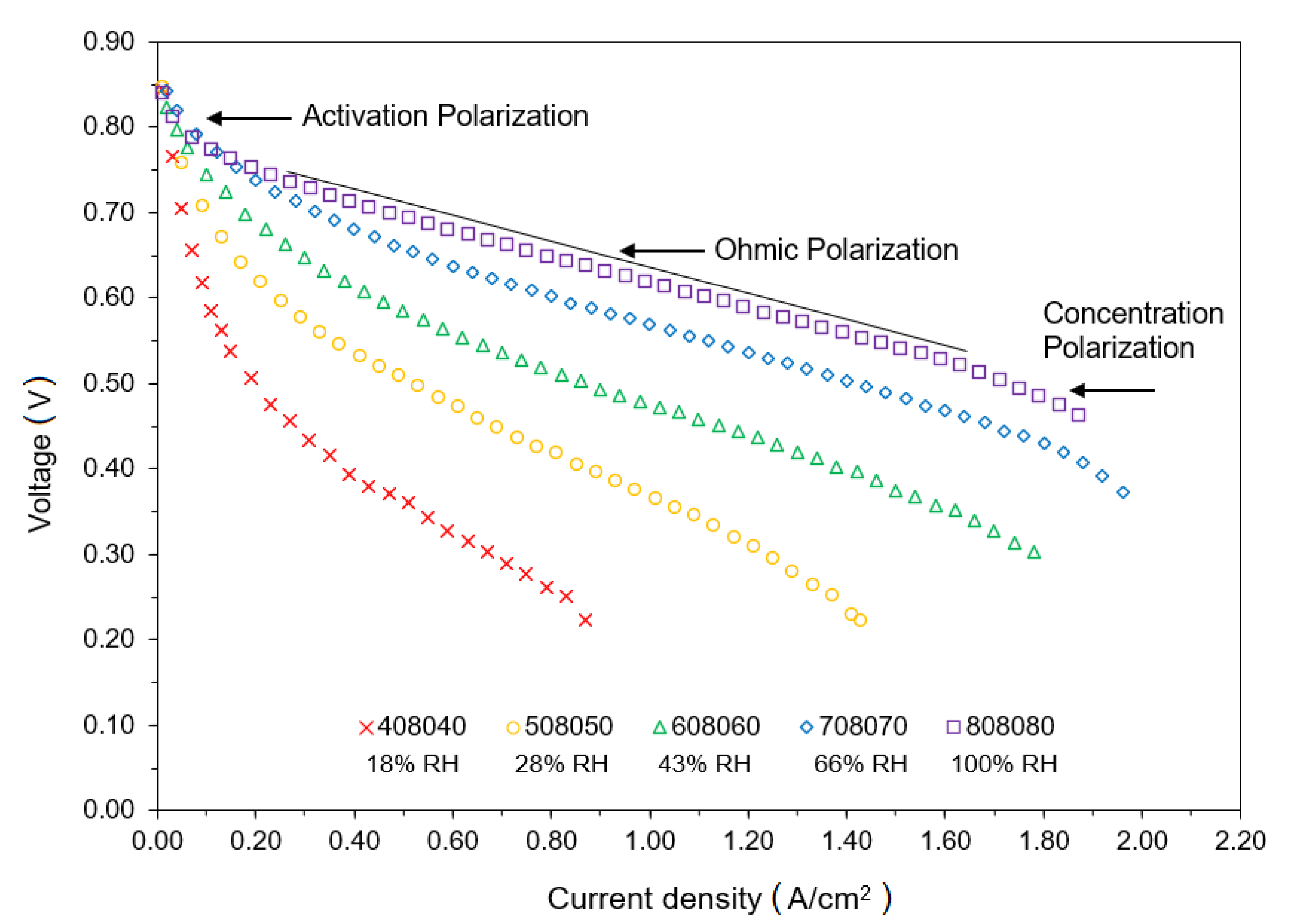
6.1. RH Impact on Performance of a PEFC

The polarization curve is a characteristic performance curve of a PEFC that shows the operating range according to the independent variables settled. Each polarization curve is composed of three defined polarization regions: activation, ohmic, and concentration. The activation polarization zone is characterized by a rapid voltage drop at the beginning of the curve. It is produced by irreversibilities that PEFC has to overcome to operate in a stable form. The irreversibilities are the back diffusion and crossover fuel, which take place in the polymeric membrane. The next region is the ohmic polarization zone. Its name is attributed to ohm’s law; this zone is characterized as the fuel cell voltage is proportional to the current density, and its slope depicts the cell’s resistance. Finally, it is the concentration polarization zone; to enter this region, the polarization curve suffers a second rapid drop. It is produced commonly due to the lack of fuel at the catalyst layer. At high current density, the water generation within the PEFC increases, obstructing the porous media. Thus, the electrochemical reactions can not hold, and the performance drops sharply.
In Figure 3, the polarization curves obtained in the present study are shown for different RH of the reactant gases. RH is one of the most important independent variables that affect the performance of a PEFC, as shown in studies [37,38,59]. It is caused mainly for the polymeric membrane used in PEFC. The membrane performance is higher when the RH of the gases is close to 100%, while the performance is lower when the RH falls in low values. This is the reason because the reactant gases have to enter humidified inside the PEFC. However, there are applications for PEFC that need to operate at low RH; for this, studies to analyze and quantify the effect of this variable are required.
As shown in Figure 3, the polarization curve with the best performance is tagged with 808080, i.e., 100% RH. It is reached when the temperature of the reactant gases is equal to the temperature of the PEFC. In this case, the maximum current density for the PEFC is around 2.0 A/cm2. However, the recommended range to operate is between 0.2 up to 1.8 A/cm2, which depicts the ohmic polarization zone, i.e., the more stable region for operating in real applications. Then, it can be noted that the PEFC performance decreases when the RH decreases too. The lower RH presented in this study is when the temperature of the reactant gases is 40 ° C, while the cell’s temperature is maintained at 80 ° C. In this regard, a 16% RH value is obtained. The maximum current density with previously settled conditions is around 0.9 A/cm2. At the same time, its ohmic polarization zone is a little unstable and has a reduced operating range concerning the other curves. This will be discussed in the later section. In addition, there is a difference of 1.4 A/cm2, comparing the maximum current densities for 100% RH and 16% RH. This indicates the significant influence of HR on the performance of a PEFC.

6.2. Sparsity and Noise of Experimentally Collected Data

All polarization curves were obtained using the same experiment configuration, where the sample rate to collect data was 0.25 A/s. The test range goes from 0 to 50 A, which is the current load maximum limit of the system. Data are obtained until the experiment drops on its own due to the performance based on conditions settled. In addition, the threshold voltage set up is 0.20 V for all cases. This setup of parameters is according to [40]. When the RH has low values, data are obtained in lower amounts due to decreased operating efficiency, which is considered sparsity in data. Hence, at low RH, the threshold voltage is probably reached for low current density, making the test stop because PEFC would be working in critical conditions.
On the other hand, concerning noise in data, Table 4 shows the aTV computed for all collected subsets, where each one is associated with a RH.
At first glance, in Figure 3, not much could be inferred about the data dispersion. However, the aTV parameter shows that there is greater dispersion for curves with lower RH than when working with higher RH. This means that, with a higher value of RH, the experiment becomes more efficient and can reach 2.0 A/cm2 without stopping due to a voltage drop, which is very usual at low RH values. Furthermore, the prediction of the OAs at a low value of RH could cause less efficient results than at a high value of RH. As there are less data and more noise, it could originate trends not so fitted with the experimental curve compared to the predicted curves at low and high RH.

6.3. Computed Unknown Parameters

Before computing the parameters, it is important to mention that the unknown parameters can be influenced by temperature, relative humidity, the stoichiometric ratio of the feed gases, and the composition or microstructural configuration of the MEA. For each configuration of the aforementioned variables, the unknown parameters will have their corresponding associated values. Despite this, the microstructural configuration does not change in the current study since the MEA used was the same in all tests. Furthermore, the stoichiometric ratio remained constant in all tests. Hence, in the current study, the primary variable that determines the parameters is the relative humidity.
With the described parameters in Section 5.3, OAs were performed and the unknown parameters are obtained according to the different RH employed in each experiment. To make this methodology reproducible and more statistically significant, the OAs were replicated 100 times. It was similarly done in the described tests in the articles corresponding to each different OA. Next, Table 5, Table 6, Table 7, Table 8 and Table 9 resume the computed unknown parameters, the calculated prediction errors for each OA, which are defined by the RMSE metric, the information about the training time elapsed by the OAs, and the computed global optima (GO), during those training stages.
As observed, for all OAs, the error is computed at different RH percentages. Comparing the algorithm, the efficiency of the OA is contrasted in both training error and training time. As it has been mentioned, NNA is one of the most recent proposals in the OA field, which has shown a better accuracy over other OAs, considering variables of analysis like the training error and training time.
Following that hypothesis, in this work, NNA once again shows an advantage in general over BSA, ALO, I-GWO, and MVO. For example, for RH values such as 18%, 66%, and 100%, the training error is the lowest, while, in other RH values like 28% and 43%, the training error of I-GWO or BSA is lower than NNA. If the training time is analyzed, in the two most recently mentioned RH percentages, NNA is better since it takes less time to train the model. Thus, in a nutshell, NNA applied to this optimization problem shows excellent performance, considering that these experiments have been developed under different operation conditions.
Another point of analysis of OAs is about the convergence curves, which indicate how the OA has optimized the unknown parameters to reach the global minimum or maximum of its cost function through the training in the established epochs or iterations. In this case, Figure 4 shows the convergence curves for all trained OAs, considering the performed experiment under 100% RH, where it is clear that all curves reach the convergence along the iterations; nevertheless, the way in which each OA operates in its search space is different, and it varies along the iterations as it can be seen in Figure 4.
Furthermore, for performance information given in the global optima reached through OAs, it is important to understand the statistical significance and level of reproducibility of the models. For instance, in the aforementioned tables, the global optima obtained along the trained OA models are similar, though the standard deviation could be high or low, which indicates that, if the standard deviation is high, it is highly likely that the model is not reproducible since, each time, the results can present large variations. Instead, if the standard deviation is low, it is highly likely that the model is reproducible, since the obtained results each time are very similar and reliable. Following this analysis, NNA shows a better advantage over the rest of the OAs in the G O s t d computed in all the trained models.
Next, Figure 5, Figure 6, Figure 7, Figure 8 and Figure 9 show the prediction curves for the best OA, i.e., in this case NNA, at different RH values.
On the other hand, in Figure 5, Figure 6, Figure 7, Figure 8 and Figure 9, the modeled polarization curves are presented according to the OA with the best performance, where it is also clear that data points do not trace a smooth curve in low RH percentages. By contrast, there is a bit of noise in the data. As the RH values increment, this noise vanishing and data points describe curves more smoothly. To justify this, it is crucial to analyze the operating conditions under the lab-scale FC test system works from a technical point of view, as it is described in Section 6.2.
The results have shown how the OAs help obtain the best parameters missing for modeling the polarization curves with a considerably reduced time since the experimental methods for obtaining the unknown parameters involve extensive time and resources consumption. Furthermore, as previously mentioned, the NNA had the best performance compared with other natural OAs, even in tests with noise (low relative humidity). Moreover, the models run in the current study yield as final results modeling polarization curves with higher accuracy that can be used in the future for designing, controlling, and simulating complex engineering problems of PEFC.

7. Conclusions

Some different OAs have been applied to this engineering problem to define the optimal values of PEFCs’ unknown parameters so correct modeling, control, and simulation can be carried out for a specific experiment related to some of the PEFCs’ applications as polarization curves. The tests are performed at different RH values to show the effectiveness of OAs for every dataset that was experimentally obtained. According to the numerical results, several conclusions can be made as shown next:
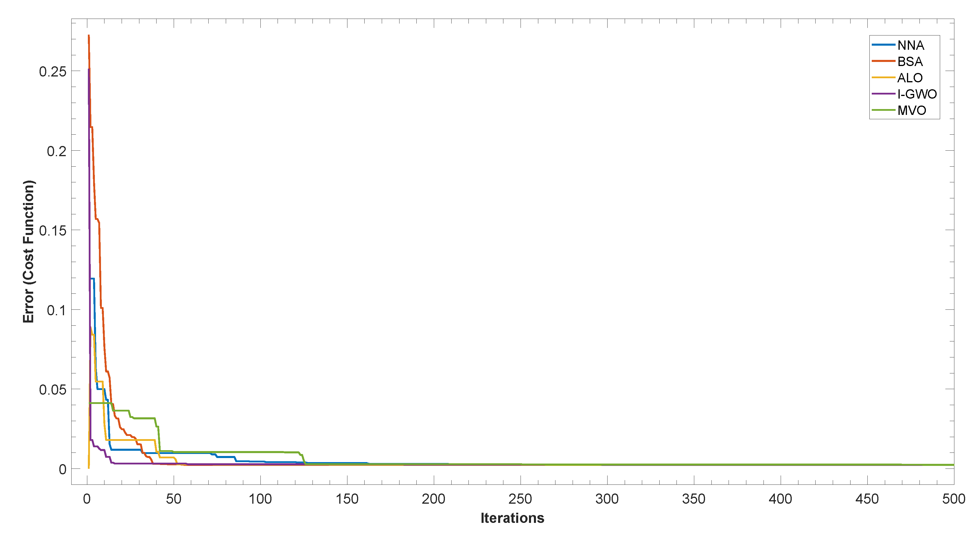
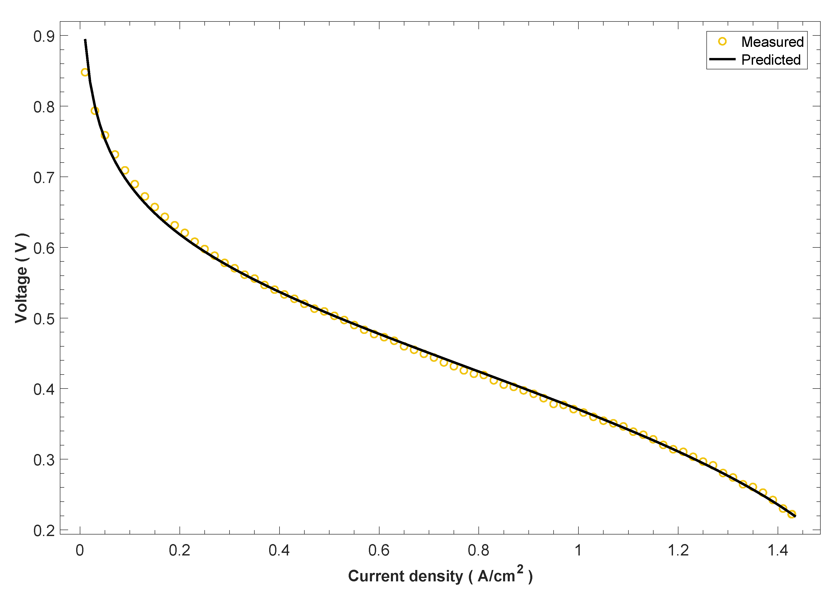
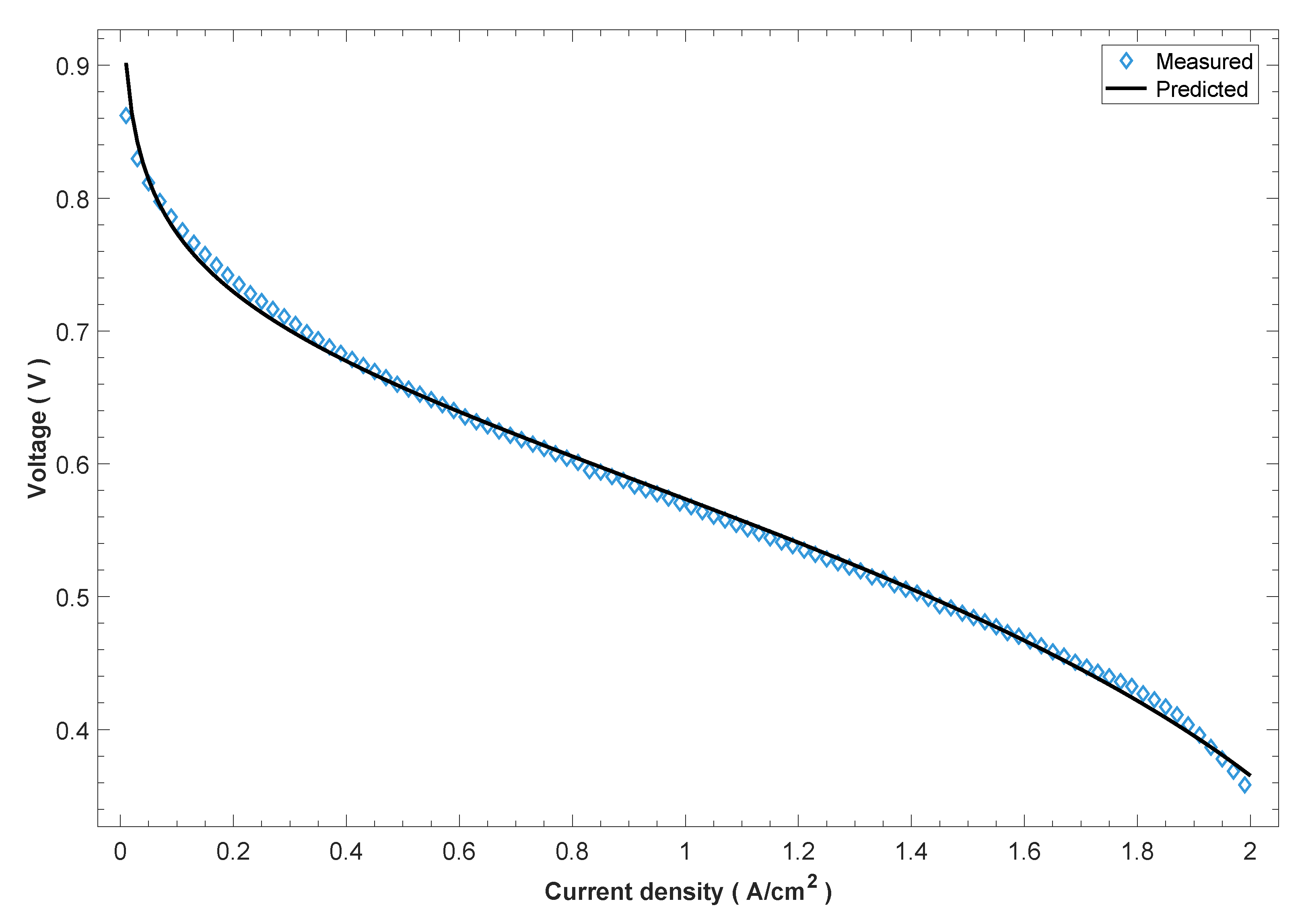
  • In all cases, for the five different OAs (NNA, MVO, BSA, ALO, and I-GWO) applied in this PEFC optimization problem, well fittings between measured and predicted voltage points are reached when using the optimal values of the unknown parameters for PEFCs.
  • Statistical performance measures have been made to evaluate the efficiency and competency of the five algorithms used to carry out this experiment, concluding that NNA proves to give the best results for the optimal values of PEFCs’ unknown parameters in almost all scenarios.
  • NNA and MVO show a better response than the other three algorithms when only referring to the training time. Although NNA optimal values are better, focusing on the metric used to measure the error between measured and predicted voltage points.
  • The optimal values for PEFCs’ unknown parameters were obtained at different RH percentages. The NNA optimizer performed the best training in three out of five scenarios, as, at RH values of 28% and 43%, I-GWO and BSA showed more accurate results when focusing on the statistical performance measures.
  • The comparisons that are properly detailed in this paper give the authors enough information to confirm and conclude that the NNA optimizer has a better performance and shows the best results, comparing it with other highlighted OAs.
Likewise, about the experimental section, a few conclusions have also been performed, as follows:
  • The polarization curves obtained show the great influence that the RH has on the performance of a PEFC, obtaining a significant decrease in range operation of 1.4 A/cm2 when the RH is modified from 100% RH to 16% RH.
  • Another RH impact on the performance of a PEFC is the increased presence of data sparsity and noise at low RH due to the PEFC works under critical operating conditions. Therefore, it also affects predicted curves that have a lower fit.
  • To sum up, the data sparsity and noise also affect OAs, since it represents a higher difficulty in finding the optimal parameters that allow for reaching the best fitting of the polarization curves to data through the PEFC mathematical model.

Author Contributions

Á.E.-D.; Methodology, Software, Validation, Formal Analysis, Writing—Review and Editing, S.E.; Methodology, Writing—Review and Editing, J.S.-V.; Methodology, Validation, Formal Analysis, Writing—Review and Editing, G.C.; Methodology, Writing—Review and Editing, M.E.-A.; Conceptualization, Methodology, Resources, Supervision, Project administration, Funding acquisition, Writing—Review and Editing. All authors have read and agreed to the published version of the manuscript.

Funding

This work has been funded by ESPOL through the grant number FIMCP-CERA-05-2017.

Institutional Review Board Statement

Not applicable.

Informed Consent Statement

Not applicable.

Data Availability Statement

The data presented in this study are available on request from the corresponding author. The data are not publicly available due to their current utilization for future works involving the authors of this paper.

Acknowledgments

The authors kindly acknowledge the support from ESPOL. Computational and physical resources provided by ESPOL are gratefully acknowledge. The support from “Decanato de Investigación” at ESPOL is also gratefully acknowledged.

Conflicts of Interest

The authors declare no conflict of interest. The founding sponsors had no role in the design of the study; in the collection, analyses, or interpretation of the data; in the writing of the manuscript, and in the decision to publish the results.

References

  1. Gutiérrez-Martín, F.; Da Silva-Álvarez, R.A.; Montoro-Pintado, P. Effects of wind intermittency on reduction of CO2 emissions: The case of the Spanish power system. Energy 2013, 61, 108–117. [Google Scholar] [CrossRef]
  2. Rodriguez, C.; Alaswad, A.; Benyounis, K.Y.; Olabi, A.G. Pretreatment techniques used in biogas production from grass. Renew. Sustain. Energy Rev. 2017, 68, 1193–1204. [Google Scholar] [CrossRef] [Green Version]
  3. Wang, K.; Wu, H.; Wang, D.; Wang, Y.; Tong, Z.; Lin, F.; Olabi, A.G. Experimental study on a coiled tube solar receiver under variable solar radiation condition. Sol. Energy 2015, 122, 1080–1090. [Google Scholar] [CrossRef]
  4. Olabi, A.G. Renewable energy and energy storage systems. Energy 2017, 136, 54. [Google Scholar] [CrossRef]
  5. Kelly-Yong, T.L.; Lee, K.T.; Mohamed, A.R.; Bhatia, S. Potential of hydrogen from oil palm biomass as a source of renewable energy worldwide. Energy Policy 2007, 35, 5692–5701. [Google Scholar] [CrossRef]
  6. Wilberforce, T.; Alaswad, A.; Palumbo, A.; Dassisti, M.; Olabi, A.G. Advances in stationary and portable fuel cell applications. Int. J. Hydrogen Energy 2016, 41, 16509–16522. [Google Scholar] [CrossRef] [Green Version]
  7. Zappa, W.; Junginger, M.; van den Broek, M. Is a 100% renewable European power system feasible by 2050? Appl. Energy 2019, 233–234, 1027–1050. [Google Scholar] [CrossRef]
  8. Spiegel, C.; York, N.; San, C.; Lisbon, F.; Madrid, L.; City, M.; New, M.; San, D.; Singapore, J.S.; Toronto, S. Designing and Building Fuel Cells Library of Congress Cataloging-in-Publication Data; Mc Graw Hill: New York, NY, USA, 2021; p. 417. ISBN 0-07-148977-0. [Google Scholar]
  9. Sharaf, O.Z.; Orhan, M.F. An overview of fuel cell technology: Fundamentals and applications. Renew. Sustain. Energy Rev. 2014, 32, 810–853. [Google Scholar] [CrossRef]
  10. Von Spakovsky, M.R.; Olsommer, B. Fuel cell systems and system modeling and analysis perspectives for fuel cell development. Energy Convers. Manag. 2002, 43, 1249–1257. [Google Scholar] [CrossRef]
  11. Carrette, L.; Friedrich, K.A.; Stimming, U. Fuel Cells: Principles, Types, Fuels, and Applications. ChemPhysChem 2000, 1, 162–193. [Google Scholar] [CrossRef]
  12. Santarelli, M.G.; Torchio, M.F. Experimental analysis of the effects of the operating variables on the performance of a single PEMFC. Energy Convers. Manag. 2007, 48, 40–51. [Google Scholar] [CrossRef]
  13. Santarelli, M.G.; Torchio, M.F.; Cochis, P. Parameters estimation of a PEM fuel cell polarization curve and analysis of their behavior with temperature. J. Power Sources 2006, 159, 824–835. [Google Scholar] [CrossRef]
  14. Zhang, Q.; Lin, R.; Técher, L.; Cui, X. Experimental study of variable operating parameters effects on overall PEMFC performance and spatial performance distribution. Energy 2016, 115, 550–560. [Google Scholar] [CrossRef]
  15. Basu, S. Recent Trends in Fuel Cell Science and Technology; Springer: New York, NY, USA, 2021; p. 375. ISBN 0-387-35537-5. [Google Scholar]
  16. Yang, S.; Chellali, R.; Lu, X.; Li, L.; Bo, C. Modeling and optimization for proton exchange membrane fuel cell stack using aging and challenging P systems based optimization algorithm. Energy 2016, 109, 569–577. [Google Scholar] [CrossRef]
  17. Encalada, Á.; Espinoza-Andaluz, M. Compression Effects on Mass Transport Phenomena in digitally generated PEFC Gas Diffusion Layers by using OpenPNM. In Proceedings of the 2020 IEEE ANDESCON, Quito, Ecuador, 13–16 October 2020; pp. 1–6. [Google Scholar] [CrossRef]
  18. Fawzi, M.; El-Fergany, A.A.; Hasanien, H.M. Effective methodology based on neural network optimizer for extracting model parameters of PEM fuel cells. Int. J. Energy Res. 2019, 43, 8136–8147. [Google Scholar] [CrossRef]
  19. Priya, K.; Sathishkumar, K.; Rajasekar, N. A comprehensive review on parameter estimation techniques for Proton Exchange Membrane fuel cell modelling. Renew. Sustain. Energy Rev. 2018, 93, 121–144. [Google Scholar] [CrossRef]
  20. Correa, J.; Farret, F.; Popov, V.; Simoes, M. Sensitivity analysis of the modeling parameters used in Simulation of proton exchange membrane fuel cells. IEEE Trans. Energy Convers. 2005, 20, 211–218. [Google Scholar] [CrossRef]
  21. Jia, J.; Li, Q.; Wang, Y.; Cham, Y.T.; Han, M. Modeling and Dynamic Characteristic Simulation of a Proton Exchange Membrane Fuel Cell. IEEE Trans. Energy Convers. 2009, 24, 283–291. [Google Scholar] [CrossRef]
  22. Djilali, N. Computational modelling of polymer electrolyte membrane (PEM) fuel cells: Challenges and opportunities. Energy 2007, 32, 269–280. [Google Scholar] [CrossRef]
  23. El-Hay, E.; El-Hameed, M.; El-Fergany, A. Steady-state and dynamic models of solid oxide fuel cells based on Satin Bowerbird Optimizer. Int. J. Hydrogen Energy 2018, 43, 14751–14761. [Google Scholar] [CrossRef]
  24. Ettihir, K.; Boulon, L.; Becherif, M.; Agbossou, K.; Ramadan, H. Online identification of semi-empirical model parameters for PEMFCs. Int. J. Hydrogen Energy 2014, 39, 21165–21176. [Google Scholar] [CrossRef]
  25. Tahmasbi, A.A.; Hoseini, A.; Roshandel, R. A new approach to multi-objective optimisation method in PEM fuel cell. Int. J. Sustain. Energy 2015, 34, 283–297. [Google Scholar] [CrossRef]
  26. Petrescu, S.; Petre, C.; Costea, M.; Malancioiu, O.; Boriaru, N.; Dobrovicescu, A.; Feidt, M.; Harman, C. A methodology of computation, design and optimization of solar Stirling power plant using hydrogen/oxygen fuel cells. Energy 2010, 35, 729–739. [Google Scholar] [CrossRef]
  27. Li, J.; Gao, N.; Cao, G.Y.; Zhu, X.J. Modeling of DIR-SOFC Based on Particle Swarm Optimization-Wavelet Network. In Advanced Materials Research; Advanced Materials and Processes II; Trans Tech Publications Ltd.: Freienbach, Switzerland, 2012; Volume 557, pp. 2202–2207. [Google Scholar] [CrossRef]
  28. Abualigah, L.; Shehab, M.; Alshinwan, M.; Mirjalili, S.; Elaziz, M.A. Ant Lion Optimizer: A Comprehensive Survey of Its Variants and Applications. Arch. Comput. Methods Eng. 2020, 28, 1397–1416. [Google Scholar] [CrossRef]
  29. Priya, K.; Sudhakar Babu, T.; Balasubramanian, K.; Sathish Kumar, K.; Rajasekar, N. A novel approach for fuel cell parameter estimation using simple Genetic Algorithm. Sustain. Energy Technol. Assess. 2015, 12, 46–52. [Google Scholar] [CrossRef]
  30. Gong, W.; Cai, Z. Accelerating parameter identification of proton exchange membrane fuel cell model with ranking-based differential evolution. Energy 2013, 59, 356–364. [Google Scholar] [CrossRef]
  31. Ye, M.; Wang, X.; Xu, Y. Parameter identification for proton exchange membrane fuel cell model using particle swarm optimization. Int. J. Hydrogen Energy 2009, 34, 981–989. [Google Scholar] [CrossRef]
  32. Fathy, A.; Rezk, H. Multi-verse optimizer for identifying the optimal parameters of PEMFC model. Energy 2018, 143, 634–644. [Google Scholar] [CrossRef]
  33. Ali, M.; El-Hameed, M.; Farahat, M. Effective parameters’ identification for polymer electrolyte membrane fuel cell models using grey wolf optimizer. Renew. Energy 2017, 111, 455–462. [Google Scholar] [CrossRef]
  34. Khodaei, H.; Hajiali, M.; Darvishan, A.; Sepehr, M.; Ghadimi, N. Fuzzy-based heat and power hub models for cost-emission operation of an industrial consumer using compromise programming. Appl. Therm. Eng. 2018, 137, 395–405. [Google Scholar] [CrossRef]
  35. Cao, Y.; Kou, X.; Wu, Y.; Jermsittiparsert, K.; Yildizbasi, A. PEM fuel cells model parameter identification based on a new improved fluid search optimization algorithm. Energy Rep. 2020, 6, 813–823. [Google Scholar] [CrossRef]
  36. Mirjalili, S.; Mirjalili, S.M.; Lewis, A. Grey Wolf Optimizer. Adv. Eng. Softw. 2014, 69, 46–61. [Google Scholar] [CrossRef] [Green Version]
  37. Santana, J.; Espinoza-Andaluz, M.; Li, T.; Andersson, M. A Detailed Analysis of Internal Resistance of a PEFC Comparing High and Low Humidification of the Reactant Gases. Front. Energy Res. 2020, 8, 1–12. [Google Scholar] [CrossRef]
  38. Espinoza-Andaluz, M.; Santana, J.; Andersson, M. Empirical correlations for the performance of a PEFC considering relative humidity of fuel and oxidant gases. Int. J. Hydrogen Energy 2020, 45, 29763–29773. [Google Scholar] [CrossRef]
  39. Associates, S. Fuel Cell Test System Operating Manual 850C; Scribner Associates, Inc.: Southern Pines, NC, USA, 2021; Volume 1, pp. 1–66. [Google Scholar]
  40. Cooper, K.; Ramani, V.; Fenton, J.M.; Kurtz, H.R. Experimental Methods and Data Analyses for Polymer Electrolyte Fuel Cells; Scribner Associates, Inc.: Southern Pines, NC, USA, 2005; p. 119. [Google Scholar]
  41. Milewski, J.; Szczęśniak, A.; Szablowski, L. A discussion on mathematical models of proton conducting Solid Oxide Fuel Cells. Int. J. Hydrogen Energy 2019, 44, 10925–10932. [Google Scholar] [CrossRef]
  42. Bavarian, M.; Soroush, M. Mathematical modeling and steady-state analysis of a proton-conducting solid oxide fuel cell. J. Process. Control 2012, 22, 1521–1530. [Google Scholar] [CrossRef]
  43. Mann, R.F.; Amphlett, J.C.; Hooper, M.A.; Jensen, H.M.; Peppley, B.A.; Roberge, P.R. Development and application of a generalized steady-state electrochemical model for a PEM fuel cell. J. Power Sources 2000, 86, 173–180. [Google Scholar] [CrossRef]
  44. Squadrito, G.; Maggio, G.; Passalacqua, E.; Lufrano, F.; Patti, A. Empirical equation for polymer electrolyte fuel cell (PEFC) behaviour. J. Appl. Electrochem. 1999, 29, 1449–1455. [Google Scholar] [CrossRef]
  45. El-Fergany, A.A. Extracting optimal parameters of PEM fuel cells using Salp Swarm Optimizer. Renew. Energy 2018, 119, 641–648. [Google Scholar] [CrossRef]
  46. Cheng, J.; Zhang, G. Parameter fitting of PEMFC models based on adaptive differential evolution. Int. J. Electr. Power Energy Syst. 2014, 62, 189–198. [Google Scholar] [CrossRef]
  47. Kandidayeni, M.; Macias, A.; Khalatbarisoltani, A.; Boulon, L.; Kelouwani, S. Benchmark of proton exchange membrane fuel cell parameters extraction with metaheuristic optimization algorithms. Energy 2019, 183, 912–925. [Google Scholar] [CrossRef]
  48. Agwa, A.M.; El-Fergany, A.A.; Sarhan, G.M. Steady-State Modeling of Fuel Cells Based on Atom Search Optimizer. Energies 2019, 12, 1884. [Google Scholar] [CrossRef] [Green Version]
  49. Rao, Y.; Shao, Z.; Ahangarnejad, A.H.; Gholamalizadeh, E.; Sobhani, B. Shark Smell Optimizer applied to identify the optimal parameters of the proton exchange membrane fuel cell model. Energy Convers. Manag. 2019, 182, 1–8. [Google Scholar] [CrossRef]
  50. Bozorg-Haddad, O. Advanced Optimization by Nature-Inspired Algorithms; Springer: Berlin/Heidelberg, Germany, 2018. [Google Scholar]
  51. Abd-Alsabour, N. Nature as a Source for Inspiring New Optimization Algorithms. In Proceedings of the 9th International Conference on Signal Processing Systems, ICSPS, Auckland, New Zealand, 27–30 November 2017; Association for Computing Machinery: New York, NY, USA, 2017; pp. 51–56. [Google Scholar] [CrossRef]
  52. Nadimi-Shahraki, M.H.; Taghian, S.; Mirjalili, S. An improved grey wolf optimizer for solving engineering problems. Expert Syst. Appl. 2021, 166, 113917. [Google Scholar] [CrossRef]
  53. Mirjalili, S. The Ant Lion Optimizer. Adv. Eng. Softw. 2015, 83, 80–98. [Google Scholar] [CrossRef]
  54. Anderson, T.R. Biology of the Ubiquitous House Sparrow: From Genes to Populations; Oxford University Press: Oxford, UK, 2006. [Google Scholar]
  55. Meng, X.B.; Gao, X.; Lu, L.; Liu, Y.; Zhang, H. A new bio-inspired optimisation algorithm: Bird Swarm Algorithm. J. Exp. Theor. Artif. Intell. 2016, 28, 673–687. [Google Scholar] [CrossRef]
  56. Sadollah, A.; Sayyaadi, H.; Yadav, A. A dynamic metaheuristic optimization model inspired by biological nervous systems: Neural network algorithm. Appl. Soft Comput. 2018, 71, 747–782. [Google Scholar] [CrossRef]
  57. Mirjalili, S.; Mirjalili, S.M.; Hatamlou, A. Multi-Verse Optimizer: A Nature-Inspired Algorithm for Global Optimization. Neural Comput. Appl. 2016, 27, 495–513. [Google Scholar] [CrossRef]
  58. Bally, V.; Caramellino, L. Total variation distance between stochastic polynomials and invariance principles. Ann. Probab. 2019, 47, 3762–3811. [Google Scholar] [CrossRef] [Green Version]
  59. Wang, B.; Lin, R.; Liu, D.; Xu, J.; Feng, B. Investigation of the effect of humidity at both electrode on the performance of PEMFC using orthogonal test method. Int. J. Hydrogen Energy 2019, 44, 13737–13743. [Google Scholar] [CrossRef]
Figure 1. Representative internal scheme of a Polymer Electrolyte Fuel Cell (PEFC) [37].
Energies 14 05631 g001
Figure 2. General flowchart for OAs, considering the main steps of the optimization procedure.
Energies 14 05631 g002
Figure 3. Polarization curves obtainedexperimentally: cell voltage as a function of current density for different relative humidities.
Energies 14 05631 g003
Figure 4. Convergence curves for the trained OAs, considering 100% RH.
Energies 14 05631 g004
Figure 5. Modeled polarization curve using the computed unknown parameters through NNA, at 18% RH.
Energies 14 05631 g005
Figure 6. Modeled polarization curve using the computed unknown parameters through NNA, at 28% RH.
Energies 14 05631 g006
Figure 7. Modeled polarization curve using the computed unknown parameters through NNA, at 43% RH.
Energies 14 05631 g007
Figure 8. Modeled polarization curve using the computed unknown parameters through NNA, at 66% RH.
Energies 14 05631 g008
Figure 9. Modeled polarization curve using the computed unknown parameters through NNA, at 100% RH.
Energies 14 05631 g009
Table 1. Upper and lower limitsfor unknown parameters of a PEFC mathematical model.
Limits ξ 1 ξ 3 (1 × 10 5 ) ξ 4 (1 × 10 5 ) λ R c  (m Ω ) β
Upper−0.85329.80−9.5423.000.800.5000
Lower−1.19973.60−26.0013.000.100.0136
Table 2. RH and J m a x values for the different gases temperature tested in the experiments.
Gas Temperature ( ° C)RH (%) J max (A/cm2)
4018.001.0277
5027.701.6372
6042.622.1890
7065.572.3779
80100.002.4529
Table 3. Input parameters for OAs (* means NOT APPLICABLE).
OAMpd c 1 c 2 a 1 a 2 FQ
NNA [56]500506*****
BSA [55]5005061.51.5113
ALO [53]500506*****
I-GWO [52]500506*****
MVO [57]500506*****
Table 4. Noise metric applied to measured voltage points in each polarization curve.
RH (%)18.0027.7042.6265.57100.00
aTV (1 × 10⁻³)7.5504.3513.0552.5652.028
Table 5. Unknown parameters computed and performance information for the modeled polarization curve at 18% RH.
ParametersNNABSAALOI-GWOMVO
ξ 1 −1.1149−1.1149−1.1994−1.1154−1.1997
ξ 3 ( 1 × 10 5 ) 9.79999.79997.91549.79187.9091
ξ 4 ( 1 × 10 5 ) −25.9999−25.9999−25.9999−25.9999−25.9999
λ 13.000013.000013.000013.000413.0000
R c (m Ω )0.80000.80000.80000.79970.8000
β 0.06450.06450.06450.064400.0645
ϵ ( 1 × 10 2 ) 1.86641.86641.86651.86641.8665
t t r a i n i n g (s)35.816128.142734.891787.344930.7480
G O b e s t ( 1 × 10 2 ) 3.13513.13513.13533.13523.1353
G O w o r s t ( 1 × 10 2 ) 3.13533.40243.63503.13763.3613
G O s t d ( 1 × 10 7 ) 7.29809504.980011,392.577048.98205320.4450
Table 6. Unknown parameters computed and performance information for the modeled polarization curve at 28% RH.
ParametersNNABSAALOI-GWOMVO
ξ 1 −1.0192−1.0320−1.1828−1.1194−1.1997
ξ 3 ( 1 × 10 5 ) 9.79979.51296.14907.56095.7752
ξ 4 ( 1 × 10 5 ) −24.4553−24.4632−24.4484−24.4732−24.4214
λ 14.271714.211022.290314.206414.1801
R c (m Ω )0.80000.79940.80000.79930.8000
β 0.05820.05780.05870.057790.0579
ϵ ( 1 × 10 3 ) 5.84805.84905.84905.84905.8500
t t r a i n i n g (s)68.968388.901982.6906201.310280.6157
G O b e s t ( 1 × 10 2 ) 4.99344.99444.99494.99554.9959
G O w o r s t ( 1 × 10 2 ) 5.24596.35686.61485.10946.4502
G O s t d ( 1 × 10 7 ) 6.53554079.05204193.5260163.73204009.5830
Table 7. Unknown parameters computed and performance information for the modeled polarization curve at 43% RH.
ParametersNNABSAALOI-GWOMVO
ξ 1 −0.9891−0.9891−1.1605−1.0420−1.1997
ξ 3 ( 1 × 10 5 ) 9.79999.80005.97198.61775.0981
ξ 4 ( 1 × 10 5 ) −20.3072−20.3074−20.3087−20.3098−20.2981
λ 22.999922.999923.000022.999422.6254
R c (m Ω )0.79990.79990.80000.79960.7997
β 0.07530.07530.07530.075200.07435
ϵ ( 1 × 10 2 ) 7.91207.91207.91307.91307.9190
t t r a i n i n g (s)191.0309135.0847111.0385385.0889108.358416
G O b e s t ( 1 × 10 2 ) 1.14561.14551.14581.14591.1476
G O w o r s t ( 1 × 10 2 ) 1.34511.48921.41071.15531.6837
G O s t d ( 1 × 10 7 ) 6011.38407731.13607497.3040142.40009409.8590
Table 8. Unknown parameters computed and performance information for the modeled polarization curve at 66% RH.
ParametersNNABSAALOI-GWOMVO
ξ 1 −0.9696−0.9692−1.0620−1.0076−1.1997
ξ 3 ( 1 × 10 5 ) 9.79169.79997.72408.94224.6376
ξ 4 ( 1 × 10 5 ) −15.0015−15.0028−14.9989−14.9991−15.0440
λ 22.999922.999923.000022.978523.0000
R c (m Ω )0.79990.79990.80000.79970.8000
β 0.06570.06570.06580.06570.0655
ϵ ( 1 × 10 2 ) 5.79805.79805.79905.80005.8000
t t r a i n i n g (s)298.3339141.123588.8788168.1751130.6152
G O b e s t ( 1 × 10 2 ) 0.67240.67240.67250.67280.6729
G O w o r s t ( 1 × 10 2 ) 0.94591.22069.07010.67871.1342
G O s t d ( 1 × 10 7 ) 6883.325010,564.23505710.6560116.02008616.5400
Table 9. Unknown parameters computed and performance information for the modeled polarization curve at 100% RH.
ParametersNNABSAALOI-GWOMVO
ξ 1 −0.9843−0.9843−1.1993−0.9906−1.1997
ξ 3 ( 1 × 10 5 ) 9.80009.79994.97729.66204.9669
ξ 4 ( 1 × 10 5 ) −9.5400−9.5400−9.5400−9.5413−9.5400
λ 23.000023.000023.000022.996323.0000
R c (m Ω )0.80000.79990.80000.79880.8000
β 0.07030.07030.07030.07010.0705
ϵ ( 1 × 10 3 ) 3.58403.58403.58503.58703.5850
t t r a i n i n g (s)95.481375.8022159.2261230.6826110.6548
G O b e s t ( 1 × 10 2 ) 2.38942.38942.39032.39312.3907
G O w o r s t ( 1 × 10 2 ) 3.85196.72733.98502.51455.4944
G O s t d ( 1 × 10 7 ) 3668.18607889.45203649.9570173.52805206.5160
Publisher’s Note: MDPI stays neutral with regard to jurisdictional claims in published maps and institutional affiliations.

