Abstract
Methane, as a clean energy source and a potent greenhouse gas, is produced in marine sediments by microbes via complex biogeochemical processes associated with the mineralization of organic matter. Quantitative modeling of biogeochemical processes is a crucial way to advance the understanding of the global carbon cycle and the past, present, and future of climate change. Here, we present a new approach of dynamic transport-reaction model combined with sediment deposition. Compared to other studies, since the model does not need the methane concentration in the bottom of sediments and predicts that value, it provides us with a robust carbon budget estimation tool in the sediment. We applied the model to the Blake Ridge region (Ocean Drilling Program, Leg 164, site 997). Based on seafloor data as input, our model remarkably reproduces measured values of total organic carbon, dissolved inorganic carbon, sulfate, calcium, and magnesium concentration in pore waters and the in situ methane presented in three phases: dissolved in pore water, trapped in gas hydrate, and as free gas. Kinetically, we examined the coexistence of free gas and hydrate, and demonstrated how it might affect methane gas migration in marine sediment within the gas hydrate stability zone.
1. Introduction
Marine sediments are the largest known methane reservoir on Earth [1,2,3,4]. The short-term carbon cycle is linked to the long-term geological sequestration of carbon by the organic matter mineralization/degradation and preservation in marine sediments [5,6]. One of the best ways to understand the global carbon cycle and its effects on, for instance, climate change, is to quantify the rates of biogeochemical processes in marine sediments [7]. The rate of organic matter degradation decreases with sediment depth, age [8], and quantity of metabolites [9].
A significant mass of CH4 is stored in marine gas hydrates, which are a potential energy resource [10] but also able to impact the atmospheric inputs of methane and, therefore, affect Earth’s climate [11,12,13]. Gas hydrate also affects the global carbon cycle since they hold vast quantities of carbon (~550 Gt of carbon) [14,15] and trap large amounts of free gas below the gas hydrate stability zone (GHSZ) [16]. As methane in the gas hydrate is dominantly microbial in origin [17], the study of organic matter decomposition kinetic in anoxic sediments has increased [1,18,19]. Numerical modeling can improve the insights into the physical and chemical processes of hydrate formation, which is a massive sink of carbon in sediments [20,21]. According to the thermodynamic perspective, free gas should not coexist with pore water within the GHSZ except along the triple point line [22,23,24]. Nevertheless, widespread seafloor methane venting reported in many regions of the world suggests the coexistence of free gas and hydrate in those places [25,26,27,28,29,30,31,32,33,34]. Thermal anomalies [35], salinity [36], capillarity [37], and crustal fingering [38] are some explanations for these field observations. Although many studies have addressed this subject from the thermodynamic point of view, few efforts have been devoted to understanding gas hydrate systems kinetics, which facilitates the free gas flow through GHSZ.
Since marine sediments are the major component of the global carbon cycle [2,4] and they have significant impacts on the oceans and sediment chemistry, and Earth’s climate, this study has focused on dynamic modeling of sedimentary organic matter mineralization and the generation and consumption (via sulfate reduction) of methane in sediments. Data obtained from the Ocean Drilling Program (ODP), in the Blake Ridge region, in the North Atlantic U.S. margin (Leg 164, site 997) was used to validate the model. The current study’s approach is to use a new numerical model to enhance the general understanding of biogeochemical processes by considering progressive sedimentation over time and provide a more reliable dynamic approximation of processes in the marine sediments. In contrast with other studies [1,4,6,9,12,19,39,40,41,42,43,44], which used the data of seafloor and bottom of sediments, the major advantages of our transport-reaction model are using the seafloor data as the only input and simulating sedimentation over time with progressive compaction of sediments. Since most of the time, it is hard or impossible to obtain the data in the deeper part of sediments, in this model, we provide a unique tool to predict methane in all phases (pore water, gas hydrate, and free gas), in addition to the concentration of sulfate, dissolved inorganic carbon, calcium, and magnesium in pore water. Furthermore, applying our model in different areas makes it possible to have a reliable prediction of the amount of methane formed in sedimentary basins, even with limited available data. Moreover, by changing the input data (such as POC and sedimentation rate) with time, it is possible to investigate their effect on biogeochemical processes. Additionally, here, we address the free gas and hydrate coexistence within the GHSZ from the kinetic perspective, which could be a new direction for future research in this area.
The rest of the paper is organized as follows. In Section 2, data source and numerical modeling of solid, dissolved, and gas species are explained. The results of simulation and comparison with available data as well as discussion are presented in Section 3. The final section summarizes the main conclusions obtained through this study.
2. Materials and Methods
2.1. Data Source
Modeling was done using available data from Janus database (http://www-odp.tamu.edu/database/), which stores data for ODP. According to the excellent pore water data set, we applied our model on site 997, Leg 164 (Blake Ridge, North Atlantic U.S. margin).
Site 997 was drilled at the Blake Ridge crest, a large contourite system [45] located in the North Atlantic U.S. margin (Figure 1). This site was selected to validate our numerical model results due to the availability of high-resolution pore water chemistry data, the presence of gas hydrate, and abundant methane of microbial origin [46]. Well-developed bottom simulating reflections (BSR) are recognized in seismic sections in the area and are interpreted as the result of free gas accumulation below the GHSZ [47]. The drilled deposits consist of Holocene to late Miocene, light gray and greenish gray, fine-grained (clay) sediment with abundant (up to 50 wt%) authigenic carbonate, which occurs as nodules and concentrated beds mostly between 50–100 m below seafloor (mbsf) and >500 mbsf (Figure 1). The occurrence of dispersed gas hydrate was reported between 180–450 mbsf, and a large piece (15 cm long) was recovered at 331 mbsf.
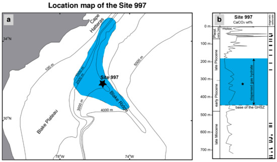
Figure 1.
(a) Location map of the site 997 drilled during ODP leg 164 in the Blake Ridge area in the North Atlantic US coast. The blue area marks the occurrence of bottom simulating reflections mapped in the area (modified from Fehn et al. [48]). (b) Composed core-log for site 997 showing calcium carbonate (wt%) in sediments. Ellipses and bars indicate the position of carbonate nodules and carbonate beds, respectively (modified from Paull et al. [49]). The blue area shows the depth range for the occurrence of dispersed gas hydrate in sediments, and the star shows the location of a 15 cm long gas hydrate piece.
2.2. Numerical Modeling
A dynamic numerical transport-reaction model [50] is applied to simulate particulate organic matter mineralization in marine sediments over time, under anoxic conditions. In this study, sediment deposition with its physical properties is reconstructed over time using sedimentation rate, geothermal gradient (Table 1), and compaction. The model calculates the spatial and temporal evolution of ten variables, i.e., concentration versus depth profiles of four solid species: (1) particulate organic carbon (POC), (2) calcium carbonate (CaCO3), (3) magnesium carbonate (MgCO3), and (4) gas hydrate (GH); five dissolved species: (5) sulfate (SO42−), (6) methane (CH4), (7) dissolved inorganic carbon (DIC), (8) calcium (Ca2+), and (9) magnesium (Mg2+), and one gas species: (10) methane. Organic matter degradation, sulfate reduction, methanogenesis, anaerobic oxidation of methane (AOM), carbonate precipitation, and methane hydrate formation and dissociation are the main processes considered in the model.

Table 1.
Parameters used in the model.
The model solves the partial differential equation for dissolved species (1), solids (2), and gas (3) based on the classical approach used in early diagenesis modeling [7,9,52]
where is time, is depth in the sediment, is the concentration of dissolved species in pore water, is the porosity, is the molecular diffusion coefficient in pore water corrected for tortuosity, sediment temperature, salinity, and pore water viscosity, is the burial velocity of solutes, is the concentration of solids in dry sediments, is the burial velocity of solids, is the concentration of free gas (normalized to pore water), is the apparent gas diffusion coefficient, is the relative velocity of ascending gas, and stands for the reactions occurring in the sediment column. The decrease in porosity with sediment depth, advective transport of solids and solutes via burial, and steady-state compaction are considered in the model. The model assumes negligible bioturbation and bioirrigation since these are typically confined to the upper 10–20 cm [1].
Our model consists of a column (1D) extending from the seafloor down to a depth of 600 mbsf. Constant concentrations of dissolved species and solids were considered as the upper boundary of the column (Dirichlet boundary conditions), corresponding to the seafloor, based on their seawater concentrations. According to ODP data for POC in site 997, a function was defined for POC input with time. POC input is considered 1.6 wt% and decreases to 0.56 wt% during the last 1.5 Myr. Zero concentration gradients (Neumann boundary condition) were prescribed as the lower boundary condition (base of the model at 600 mbsf) for sulfate, calcium, and magnesium. According to the literature, there are significant gradients of methane and DIC at lower boundary conditions, indicating that dissolved species are released in deeper sediments and transported to the surface by diffusion [9]. For simplification, in most cases, they considered a constant value or zero concentration gradients at the bottom of their modeled columns [1,9,15,43,44,53]. In this study, according to the depth and time, two boundary conditions were considered because of the sedimentation evolution. According to time, before the first layer of the sediment reaches the lowest point of the modeled column, a zero concentration gradient is imposed for methane, DIC, and free gas. After that time, by extrapolating the last two points of DIC, methane, and free gas, a virtual point was considered below the last point and used for the lower boundary condition in the bottom of the modeled column (Figure 2). Therefore, these values were changing over time to have a more realistic and novel dynamic model. A detailed description of the model and the list of used parameters are given in Appendix A.
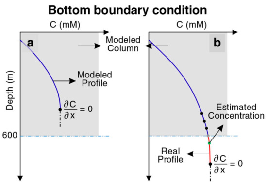
Figure 2.
Graphics illustrating the approach to define bottom boundary conditions for methane, DIC, and free gas. (a) Zero concentration gradient is imposed before the first layer of the sediment reaches the bottom of the model at a depth of 600 m. (b) Extrapolating a virtual point after the first layer passes the bottom of the model.
Simulating the growing sediment column over time with progressive compaction of sediments is a significant advantage of this model, so the model was run for 100 million years to simulate an extended period.
The ten sets of the differential equations consist of four solid species (using Equation (1)), five dissolved species (using Equation (2)), and one gas species (using Equation (3)), and were discretized using finite difference techniques and the method-of-lines [54]. The model was solved using MATLAB (R2020a, MathWorks). All modeling and calculations were done based on the data gathered from OPD site 997, Leg 164 [22,49,51].
3. Results and Discussion
3.1. Solid Phase and Pore Water Concentration
The results in the last time step of the model are shown in Figure 3. The time-lapse video of the model evolution is presented in Video S1. According to the results, sulfate concentration decreases linearly from the seafloor to the depth of 24 mbsf, which is the depth of the sulfate-methane transition (SMT). Between 0 and 18 mbsf, methane concentration is almost zero; then, its concentration rapidly increases, indicating ongoing methanogenesis and the termination of methane consumption via anaerobic oxidation of methane (AOM) in the sulfate reduction zone. In the methane profile (Figure 3b), the quantity of methane generated reaches saturation below about 170 mbsf. The higher methane values measured in the ODP reference site 997 suggest a possible dissociation of gas hydrate and methane release during core recovery.
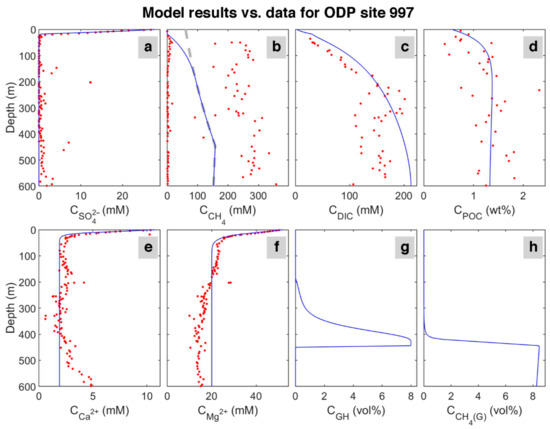
Figure 3.
Data for ODP site 997 [49] (circles) and model results (solid lines) in the last time step. The dashed line in the CH4 concentration profile indicates the saturation of methane with depth. Upper row: concentration of (a) sulfate (SO42−); (b) dissolved methane (CH4); (c) dissolved inorganic carbon (model: DIC = CO32−+HCO3−+CO2 and for data: total alkalinity + CO2) in pore water, and (d) weight percent of particulate organic carbon (POC) in sediment. Lower row: concentration of (e) calcium (Ca2+); (f) magnesium (Mg2+) in pore water, and the volume percent (calculated based on the pore volume) of (g) hydrate (GH), and (h) free gas (CH4 (G)).
Considering the seawater as the only source of calcium and magnesium in the system, the model predicts a decline in magnesium and calcium concentrations with depth due to carbonate precipitation associated with organic matter mineralization and related alkalinity increase at shallow depths below seafloor (<100 mbsf) [55]. Despite a slight increase in calcium content at about 500 mbsf in the study site, the model shows a good match with the reference site’s data. An additional source of calcium in the sediment and change in abundance of authigenic carbonate [51] could explain the difference between the model and data.
In the model, DIC results from the production of sulfate reduction, AOM, and methanogenesis [9]; however, DIC data presented here for ODP is the sum of total alkalinity, mostly produced by sulfate reduction and AOM [56], and carbon dioxide produced by methanogenesis.
3.2. Methane Phase Behavior
Figure 4 shows methane generation and sulfate consumption (via sulfate reduction and anaerobic oxidation of methane) simulated over time. At the top of the model (0–23 mbsf), most organic matter is consumed by the sulfate reduction, and the concentration of methane is nearly zero at all times. Below that depth, methane concentration slightly increases because of the onset of methanogenesis and cessation of sulfate reduction owing to sulfate depletion. After about 7 million years, more methane is produced, and the rate of AOM increases to reach an almost constant and relatively steady-state situation. As shown in Figure 4, at the beginning of the model (0–0.34 Myr), the SMT occurs in a deeper position (42 mbsf) in relation to present day (24 mbsf) because there is no methane below to be consumed via AOM which would compete for sulfate with sulfate reduction fueled by POC. As time goes on and more methane is produced, the diffusion of methane to the upper part increases and results in faster depletion in sulfate by AOM, with consequent shallowing of the SMT depth (20 mbsf). According to the decrease in POC input (98.5–100 Myr) based on the reference data for site 997, methanogenesis and sulfate reduction slightly decrease, and SMT depth increases to its present day (24 mbsf).
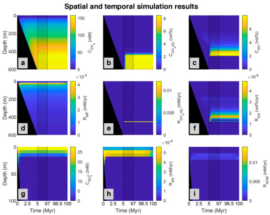
Figure 4.
Spatial and temporal results of the model for the simulated ODP site 997 [49] magnified in the first 5 Myr and the last 3 Myr (plots without magnification are presented in Appendix A, Figure A1). First row: Concentration profile of (a) Dissolved methane (CH4); (b) Methane in the gas phase (CH4 (g)); (c) Methane in hydrate phase (GH). Second row: Simulated rates of (d) Methanogenesis (MP); (e) Free gas formation (CH4 (G)), and (f) Gas hydrate formation (GH). Last row presented in shorter depth (to magnify the rate changes, which occur only at the upper part of the model): (g) Concentration profile of sulfate (SO42−); simulated rate of (h) Sulfate reduction (SR), and (i) Anaerobic oxidation of methane (AOM). The black area refers to the place where no sedimentation occurred. The area limited by dashed lines represents changes from 5 to 97 Myr.
According to the ODP report for the studied site [51], Blake Ridge contains gas hydrate, and below the GHSZ, there is an accumulation of free gas [16,57], which is produced via microbial methanogenesis [22]. According to the salinity profile, we considered up to 8% of pore volume could be occupied by gas hydrate and free gas. As shown in Figure 4, based on the model, methane produced by methanogenesis are in three phases, dissolve in pore water, as gas hydrate, and free gas. In the beginning, there is no methane in the system. By consuming all sulfate in depth, methane starts to be produced by methanogenesis. Over time, more methane is generated, and the concentration of methane in pore water increases, so it diffuses to the upper part of the column. After around three million years, when about 350 m of sediment accumulated, methane in pores below about 180 mbsf becomes supersaturated and gas hydrate forms. This depth is the upper edge of the zone with dispersed gas hydrate in sediments is described in the ODP report for site 997 [51]. As more methane is produced with time, more gas hydrate is formed. As demonstrated in the time-lapse video (Video S1), the gas hydrate produced by in situ organic matter degradation is less than 1% of the pore volume. With the continuation of deposition, gas hydrate is buried down as sedimentation proceeds and starts to dissociate when it crosses the base of the GHSZ depth, and after saturating pore water, free gas (methane bubbles) forms. On the other hand, due to the upward migration tendency of free gas by advection and diffusion, gas produced in a deeper part of the model starts to move up and enter the GHSZ to form more gas hydrate. Over time, more gas hydrate is formed and dissociated, forming a gas hydrate-rich level above and a gas-rich level below the base of the GHSZ. This contrasting horizon can be recognized in seismic sections as a bottom simulating reflections [40], which is a distinct feature in the Blake Ridge at the site 997 [47]. With time, the gas hydrate level becomes thicker and inhibits further upward gas migration, so gas accumulates below the GHSZ.
3.3. Carbon Sink
The degradation of POC, the only carbon input in the model, is transformed into methane (dissolved in pore water and as gas hydrate and free gas) and DIC, which is kept dissolved in pore water or reacts with calcium and magnesium to form carbonates [58,59]. Over time, DIC can diffuse to seawater from the top (seafloor); it can be removed from the bottom (600 mbsf) by advection (burial) or diffusion, the latter depending on the concentration profile. Dissolved methane can be removed from the bottom of the system by advection and removed or added to the system from the bottom by diffusion. Free gas can enter the system by advection and be removed or entered from the bottom by diffusion. Magnesium carbonate and calcium carbonate are in the solid phase and can be removed from the bottom by advection. There is no methane hydrate in the bottom of the modeled column because it is outside of the GHSZ (<450 mbsf). However, hydrate can be dissociated below the GHSZ, releasing methane. Time-lapse video for carbon balance is presented as Video S1. Figure 5 shows the quantity and distribution of consumed carbon per unit of the modeled column length after the last time step (i.e., 100 Myr). According to the model, about 17% of POC input is labile and consumed/mineralized in the system. From this 17%, carbon mass balance shows that DIC is the main carbon sink within the sediment (55.27%), and generated methane (dissolved, gas hydrate, and free gas) is the second carbon sink (23.13%). Methane hydrate and free gas host a minor part (0.6% and 0.9%, respectively) of the system’s total carbon. However, as shown in Figure 3, the quantity of free gas trapped below the base of the GHSZ is significantly more than the value of 0.9%, the amount of free gas produced by in situ POC degradation, which does not include the free gas entered to the modeled column from below.
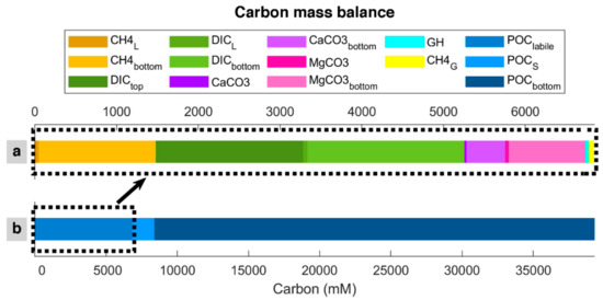
Figure 5.
Carbon mass balance calculation in the last time step of the model. (a) represents the in situ carbon sinks, while (b) is the total carbon entered the modeled column. Subscript “S”, “L”, and “G” represents concentrations in the solid phase, dissolved in pore water (liquid), and free gas produced by in situ organic matter degradation, respectively. Subscribes “top” and “bottom” stand the amount of substance that leaves the modeled column from top and bottom, respectively. Subscribe “labile” indicates the amount of converted (labile, mineralized) organic matter.
3.4. Sedimentation Rate and Initial Age of POC
To find the effect of sedimentation rate in biogeochemical processes, site 997 with constant POC at the top of the column was modeled. Since a higher sedimentation rate is equivalent to younger organic matter age [6,9,15], we considered three different initial ages with a linear function of sedimentation rate. The three sets are: (a) = 0.01 cm/yr and = 8 × 10⁵ yr (oldest), (b) = 0.02 cm/yr and = 4 × 10⁵ yr (middle-aged), and (c) = 0.04 cm/yr and = 2 × 10⁵ yr (youngest)). The results of the last time step of each set are plotted in Figure 6. By decreasing POC initial age (increasing the sedimentation rate), the organic matter becomes more reactive, and the POC degradation rate increases (according to the results, the rate of youngest POC is almost 3.73 and 1.93 times higher than the rate of the oldest and middle-aged one, respectively) results in increasing sulfate reduction and methanogenesis rates (Figure 7), and consequently, shallowing the SMT and increasing methane production (Figure 6). As methane generation increases, pore water is saturated at shallower depths, hydrate formation commences in shallower depths, and the thickness of hydrate (the supersaturation zone of methane) increases (276, 330, and 366 m for the oldest, middle-aged, and youngest, respectively), which is in general agreement with other studies [9,60]. Nevertheless, the gas hydrate average concentration decreases with an increase in sedimentation rate. Upward gas migration velocity in the lowest sedimentation rate is the highest; thus, more gas reaches GHSZ, and consequently, more hydrate is formed at the same time. On the other hand, the gas hydrate in the system with the lowest velocity is buried slower, and it leaves the GHSZ more slowly; therefore, it dissociates with a slower rate compared to the other two modeled systems. As a result, the amount of gas accumulated below the GHSZ is not proportional to the hydrate amount.
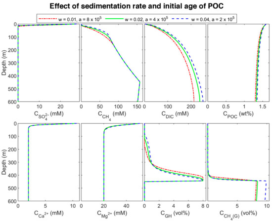
Figure 6.
Concentration profile of modeled results at different sedimentation rates and initial ages of POC in the last time step of the model.
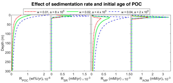
Figure 7.
Rate profiles of modeled results at different sedimentation rates and initial ages of POC in the last time step of the model.
3.5. Coexistence of Free Gas and Gas Hydrate in GHSZ
Here we propose an idea to explain the coexistence of free gas and gas hydrate in GHSZ from the kinetic perspective. The presence of materials in pore water and sediments with the ability to retard gas hydrate formation and suppress the gas hydrate growth can decline the gas hydrate formation rate (such as polysaccharides [61,62] and polyvinylcaprolactam [63] as natural and artificial kinetic hydrate inhibitors, respectively). To investigate the effect of gas hydrate formation kinetic in pores, after about 37 million years, we assumed the kinetic constant of gas hydrate decreases to 0.1, 0.01, and 0.001 of the initial value. The model was run for over 50 million years. By reducing kinetic constant, the rate of hydrate formation decreases, and since the sedimentation rate is constant, hydrate dissociates faster compared to the formation, so the pore volume occupied by gas hydrate diminishes, and the excess (supersaturation) of methane is released as bubbles (see time 38 Myr in time-lapse video in Video S2). On the other hand, as shown in Figure 8, by decreasing the gas hydrate kinetic constant, free gas below the GHSZ can migrate upwards to shallower depths. According to the model, free gas in GHSZ causes pore water to be saturated at shallower depths, increasing gas hydrate thickness and shallowing the SMT. Although the rate of AOM increases (Figure 9), it is not enough to consume all the methane, and some part of free gas can vent out the seafloor. The efficiency of AOM barrier is 97.75, 38.78, and 28.22% for the gas hydrate kinetic constants of 0.1, 0.01, and 0.001 KGH, respectively. This indicates that, by increasing the amount of free gas in top layers, AOM cannot consume all methane and leads to methane efflux to the sea-water interface. There is indication that dissolved organic carbon [64] and potentially some kinetic inhibitors may be concentrated in the sediments over time. As a suggestion, we recommend to investigate the existence of the kinetic gas hydrate inhibitors in future expeditions, especially at areas with seafloor methane venting.
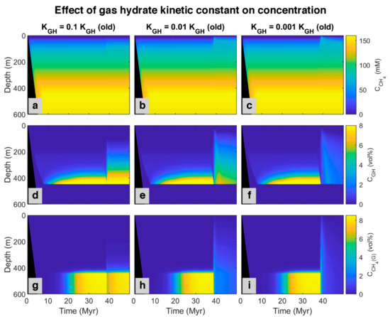
Figure 8.
Simulated spatial and temporal concentration profile at different gas hydrate kinetic constant. First row: (a–c) Dissolved methane in pore water. Second row: (d–f) Methane hosted in gas hydrate phase. Last row: (g–i) Free gas.
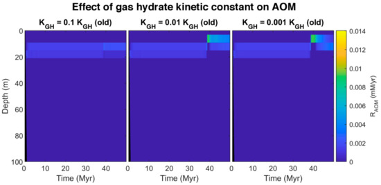
Figure 9.
Simulated rate profile of AOM at different gas hydrate kinetic constant (0–100 mbsf).
4. Conclusions
We used a dynamic model to simulate the biogeochemical process in marine sediments related to the mineralization of organic matter, including methane formation and consumption. Compared with other studies, our model predicts dissolved species’ temporal and spatial concentration in pore water, considering the seawater concentration as the top boundary condition without any subsurface information. Prediction of methane generation and consumption, SO42−, Ca2+, Mg2+, and DIC with reliable accuracy is an important achievement of our model. The model predicts that in site 997, the most gas hydrate accumulated in the sediment is formed from free gas generated by organic matter mineralization below the GHSZ. Based on our model, a massive volume of free gas below the GHSZ could migrate upwards to shallow depth if the gas hydrate formation kinetic is adequately slow.
Although our model fitted the data well by using the seafloor data as the only input, the model can be further improved by considering the energy balances to predict the effect of global warming on the methane emission in the oceans and hydrate stability.
As a future study, the model could also be used as a new tool to estimate the total carbon budget and distribution in the sediments in areas with limited data. The prediction of the methane accumulation in sediments is another clear implication of the model for exploring energy resources and understanding the past and future of Earth’s climate. Moreover, the authors are going to investigate the effect of temperature, salinity, and eutrophication on biogeochemical processes.
Supplementary Materials
The following are available online at https://www.mdpi.com/article/10.3390/en14185671/s1, Video S1: time-lapse of the model evolution, Video S2: time-lapse of coexistence of free gas and gas hydrate in GHSZ.
Author Contributions
Conceptualization, M.R.-A. and M.K.; methodology, M.R.-A. and M.A.; software, M.R.-A. and M.A.; validation, M.R.-A., M.A. and M.K.; resources, M.R.-A.; data curation, M.R.-A. and M.A.; writing—original draft preparation, M.R.-A.; writing—review and editing, M.R.-A., M.A. and M.K.; visualization, M.R.-A., M.K. and M.A.; supervision, M.K. All authors have read and agreed to the published version of the manuscript.
Funding
This research received no external funding.
Data Availability Statement
All study data are included in the article and Appendix A. The computer code is available upon reasonable requests.
Acknowledgments
We thank Linnaeus University for their support.
Conflicts of Interest
The authors declare no conflict of interest.
Appendix A
In the following, a detailed description of the model is presented in Table A1, Table A2, Table A3 and Table A4. In this study, the porosity is considered to decay exponentially with depth due to steady-state compaction [50], the porosity at depth zero (), the porosity at infinite depth (), and the attenuation coefficient () which are calculated based on the available data in the site. Decrease of the porosity because of the hydrate formation is considered in the gas hydrate stability zone by distracting the volume of hydrate from the pore volume. Burial velocity of pore water and solids are calculated based on steady-state compaction [50] and the available data is used for the sedimentation rate (). The upward velocity can be in the range of 0.005 to 30 cm yr−1 [4]. In this study, we assumed the upward velocity of gas as 0.02 cm yr−1. Molecular diffusion coefficients () are calculated in different temperature and salinity according to depth while logarithmic equation is used to consider the effect of the porosity [52].
The rate laws and expressions used in the modeling are described in Table A2 and Table A3. Modified Middelburg’s age-dependent model is used as POC degradation rate, where is inhibition constant to decrease the rate of reaction with increase in metabolites (CH4 and DIC), and a0 is the initial age of the organic matter [8,9]. The rate of sulfate reduction and methane formation are related to organic matter degradation rate, where is a Monod constant to decrease the sulfate reduction rate at low concentration of sulfate (= 1 mM) [9]. A simple second-order kinetics is used for the anaerobic oxidation of methane (AOM) [39], where is a kinetic constant. The calcium carbonate precipitation and dissolution rates are considered to depend linearly on the saturation state, where is the thermodynamic equilibrium constant modified by the pressure [39,65,66]. The magnesium carbonate precipitation and dissolution rates are assumed to depend linearly on the saturation, same as the calcium carbonate, where stands for thermodynamic equilibrium constant modified by the pressure [65,67]. In this model, whenever the concentration of dissolved methane surpassed the methane solubility (), hydrate is precipitated if it is in the hydrate stability zone; otherwise, free gas is released. The methane solubility is calculated by modified Pitzer-approach [68] and Duan-approach [69,70], in and out of hydrate stability zone, respectively. Hydrates and free gasses were allowed to dissolve in pore water if the concentration of methane is less than saturation. The kinetic parameters of the model were constrained by fitting the model to the porewater profiles (Table A4).
Table A1.
Depth-dependent parameters.
Table A1.
Depth-dependent parameters.
| Parameter | Equation |
|---|---|
| Porosity | |
| Burial velocity of solids | |
| Burial velocity of pore water | |
| Relative velocity of free gas | |
| Factor converting Cs (wt%) in Cl (mM) | |
| Molecular diffusion in sediments | |
| Factor converting wt% in vol% |
Table A2.
The rate laws used in the modeling.
Table A2.
The rate laws used in the modeling.
| Reaction | Rate Expression |
|---|---|
| POC degradation | |
| Sulfate reduction | |
| Methanogenesis | |
| Anaerobic oxidation of methane | |
| Calcium carbonate precipitation (if ) | |
| Calcium carbonate dissolution (if ) | |
| Magnesium carbonate precipitation (if ) | |
| Magnesium carbonate dissolution (if ) | |
| Hydrate formation (if ) | |
| Hydrate dissociation (if ) | |
| Free gas formation (if ) | |
| Free gas dissociation (if ) |
Table A3.
Rate expression used in the differential equations.
Table A3.
Rate expression used in the differential equations.
| Species | Rates |
|---|---|
| Particulate organic carbon (POC) | |
| Sulfate (SO42−) | |
| Methane (CH4) | |
| Dissolved inorganic carbon (DIC) | |
| Calcium (Ca2+) | |
| Magnesium (Mg2+) | |
| Calcium carbonate (CaCO3) | |
| Magnesium carbonate (MgCO3) | |
| Gas hydrate | |
| Free gas |
Table A4.
Parameters’ value derived by fitting the model to data.
Table A4.
Parameters’ value derived by fitting the model to data.
| Parameter | Units | Site 997 |
|---|---|---|
| Initial age of POC () | yr | 8 × 10⁻⁵ |
| Monod constant of POC degradation () | mM | 68 |
| Monod constant of sulfate reduction () | mM | 1 |
| Kinetic constant of AOM () | L yr−1 mmol−1 | 0.05 |
| Kinetic constant of calcium carbonate precipitation () | yr−1 wt%−1 | 10−8 |
| Kinetic constant of calcium carbonate dissolution () | yr−1 | 10−8 |
| Kinetic constant of magnesium carbonate precipitation () | yr−1 wt%−1 | 10−10 |
| Kinetic constant of magnesium carbonate dissolution () | yr−1 | 10−10 |
| Kinetic constant of hydrate formation () | yr−1 wt%−1 | 0.02 |
| Kinetic constant of hydrate dissociation () | yr−1 | 0.02 |
| Kinetic constant of free gas formation () | mM yr−1 | 20 |
| Kinetic constant of free gas dissolution () | yr−1 | 0.0002 |
| Porosity at depth zero () | – | 0.75 |
| Porosity at infinite depth () | – | 0.47 |
| Attenuation coefficient () | – | 0.00323 |

Figure A1.
Spatial and temporal results of the model for the simulated ODP site 997 [49]. First row: Concentration profile of (a) Dissolved methane (CH4); (b) Methane in the gas phase (CH4 (g)); (c) Methane in hydrate phase (GH). Second row: Simulated rate of (d) Methanogenesis (MP); (e) Free gas formation (CH4 (G)), and (f) Gas hydrate formation (GH). Last row presented in shorter depth (to magnify the rate changes): (g) Concentration profile of sulfate (SO42−); simulated rate of (h) Sulfate reduction (SR), and (i) Anaerobic oxidation of methane (AOM). The black area refers to the place where no sedimentation occurred.

References
- Hu, Y.; Luo, M.; Chen, L.; Liang, Q.; Feng, D.; Tao, J.; Yang, S.; Chen, D. Methane source linked to gas hydrate system at hydrate drilling areas of the South China Sea: Porewater geochemistry and numerical model constraints. J. Asian Earth Sci. 2018, 168, 87–95. [Google Scholar] [CrossRef]
- Buffett, B.; Archer, D. Global inventory of methane clathrate: Sensitivity to changes in the deep ocean. Earth Planet. Sci. Lett. 2004, 227, 185–199. [Google Scholar] [CrossRef]
- Kvenvolden, K.A. Gas hydrates—Geological perspective and global change. Rev. Geophys. 1993, 31, 173–187. [Google Scholar] [CrossRef]
- Regnier, P.; Dale, A.W.; Arndt, S.; LaRowe, D.E.; Mogollón, J.; Van Cappellen, P. Quantitative analysis of anaerobic oxidation of methane (AOM) in marine sediments: A modeling perspective. Earth-Sci. Rev. 2011, 106, 105–130. [Google Scholar] [CrossRef]
- Berner, R.A. Atmospheric Carbon Dioxide Levels Over Phanerozoic Time. Science 1990, 249, 1382–1386. [Google Scholar] [CrossRef] [PubMed]
- Dale, A.W.; Flury, S.; Fossing, H.; Regnier, P.; Røy, H.; Scholze, C.; Jørgensen, B.B. Kinetics of organic carbon mineralization and methane formation in marine sediments (Aarhus Bay, Denmark). Geochim. Cosmochim. Acta 2019, 252, 159–178. [Google Scholar] [CrossRef]
- Arndt, S.; Jørgensen, B.B.; LaRowe, D.E.; Middelburg, J.J.; Pancost, R.D.; Regnier, P. Quantifying the degradation of organic matter in marine sediments: A review and synthesis. Earth-Sci. Rev. 2013, 123, 53–86. [Google Scholar] [CrossRef]
- Middelburg, J.J. A simple rate model for organic matter decomposition in marine sediments. Geochim. Cosmochim. Acta 1989, 53, 1577–1581. [Google Scholar] [CrossRef]
- Wallmann, K.; Aloisi, G.; Haeckel, M.; Obzhirov, A.; Pavlova, G.; Tishchenko, P. Kinetics of organic matter degradation, microbial methane generation, and gas hydrate formation in anoxic marine sediments. Geochim. Cosmochim. Acta 2006, 70, 3905–3927. [Google Scholar] [CrossRef]
- Demirbas, A. Methane hydrates as potential energy resource: Part 1—Importance, resource and recovery facilities. Energy Convers. Manag. 2010, 51, 1547–1561. [Google Scholar] [CrossRef]
- de Garidel-Thoron, T.; Beaufort, L.; Bassinot, F.; Henry, P. Evidence for large methane releases to the atmosphere from deep-sea gas-hydrate dissociation during the last glacial episode. Proc. Natl. Acad. Sci. USA 2004, 101, 9187–9192. [Google Scholar] [CrossRef]
- Ruppel, C.D.; Kessler, J.D. The interaction of climate change and methane hydrates. Rev. Geophys. 2017, 55, 126–168. [Google Scholar] [CrossRef]
- Tinivella, U.; Giustiniani, M.; Vargas Cordero, I.D.L.C.; Vasilev, A. Gas Hydrate: Environmental and Climate Impacts. Geosciences 2019, 9, 443. [Google Scholar] [CrossRef]
- Piñero, E.; Marquardt, M.; Hensen, C.; Haeckel, M.; Wallmann, K. Estimation of the global inventory of methane hydrates in marine sediments using transfer functions. Biogeosciences 2013, 10, 959–975. [Google Scholar] [CrossRef]
- Wallmann, K.; Pinero, E.; Burwicz, E.; Haeckel, M.; Hensen, C.; Dale, A.; Ruepke, L. The Global Inventory of Methane Hydrate in Marine Sediments: A Theoretical Approach. Energies 2012, 5, 2449–2498. [Google Scholar] [CrossRef]
- Dickens, G.R.; Paull, C.K.; Wallace, P. Direct measurement of in situ methane quantities in a large gas-hydrate reservoir. Nature 1997, 385, 426–428. [Google Scholar] [CrossRef]
- Kvenvolden, K.A.; Lorenson, T.D. The Global Occurrence of Natural Gas Hydrate. Nat. Gas. Hydrates Occur. Distrib. Detect. 2001, 124, 3–18. [Google Scholar]
- Zhang, Y.; Luo, M.; Hu, Y.; Wang, H.; Chen, D. An Areal Assessment of Subseafloor Carbon Cycling in Cold Seeps and Hydrate-Bearing Areas in the Northern South China Sea. Geofluid 2019, 2019, 2573937. [Google Scholar] [CrossRef]
- Wallmann, K.; Riedel, M.; Hong, W.L.; Patton, H.; Hubbard, A.; Pape, T.; Hsu, C.W.; Schmidt, C.; Johnson, J.E.; Torres, M.E.; et al. Gas hydrate dissociation off Svalbard induced by isostatic rebound rather than global warming. Nat. Commun. 2018, 9, 83. [Google Scholar] [CrossRef]
- Zhu, H.; Xu, T.; Zhu, Z.; Yuan, Y.; Tian, H. Numerical modeling of methane hydrate accumulation with mixed sources in marine sediments: Case study of Shenhu Area, South China Sea. Mar. Geol. 2020, 423, 106142. [Google Scholar] [CrossRef]
- Malinverno, A. Marine gas hydrates in thin sand layers that soak up microbial methane. Earth Planet. Sci. Lett. 2010, 292, 399–408. [Google Scholar] [CrossRef]
- Egeberg, P.K.; Dickens, G.R. Thermodynamic and pore water halogen constraints on gas hydrate distribution at ODP Site 997 (Blake Ridge). Chem. Geol. 1999, 153, 53–79. [Google Scholar] [CrossRef]
- Zatsepina, O.Y.; Buffett, B.A. Phase equilibrium of gas hydrate: Implications for the formation of hydrate in the deep sea floor. Geophys. Res. Lett. 1997, 24, 1567–1570. [Google Scholar] [CrossRef]
- Sloan, E., Jr.; Koh, C.A. Clathrate Hydrates of Natural Gases, 3rd ed.; CRC Press: Boca Raton, FL, USA, 2008. [Google Scholar]
- Burwicz, E.; Rüpke, L. Thermal State of the Blake Ridge Gas Hydrate Stability Zone (GHSZ)—Insights on Gas Hydrate Dynamics from a New Multi-Phase Numerical Model. Energies 2019, 12, 3403. [Google Scholar] [CrossRef]
- Skarke, A.; Ruppel, C.; Kodis, M.; Brothers, D.; Lobecker, E. Widespread methane leakage from the sea floor on the northern US Atlantic margin. Nat. Geosci. 2014, 7, 657–661. [Google Scholar] [CrossRef]
- Petersen, C.J.; Bünz, S.; Hustoft, S.; Mienert, J.; Klaeschen, D. High-resolution P-Cable 3D seismic imaging of gas chimney structures in gas hydrated sediments of an Arctic sediment drift. Mar. Pet. Geol. 2010, 27, 1981–1994. [Google Scholar] [CrossRef]
- Bünz, S.; Polyanov, S.; Vadakkepuliyambatta, S.; Consolaro, C.; Mienert, J. Active gas venting through hydrate-bearing sediments on the Vestnesa Ridge, offshore W-Svalbard. Mar. Geol. 2012, 332–334, 189–197. [Google Scholar] [CrossRef]
- Gorman, A.R.; Holbrook, W.S.; Hornbach, M.J.; Hackwith, K.L.; Lizarralde, D.; Pecher, I. Migration of methane gas through the hydrate stability zone in a low-flux hydrate province. Geology 2002, 30, 327–330. [Google Scholar] [CrossRef]
- Wood, W.T.; Gettrust, J.F.; Chapman, N.R.; Spence, G.D.; Hyndman, R.D. Decreased stability of methane hydrates in marine sediments owing to phase-boundary roughness. Nature 2002, 420, 656–660. [Google Scholar] [CrossRef]
- Tréhu, A.M.; Flemings, P.B.; Bangs, N.L.; Chevallier, J.; Gràcia, E.; Johnson, J.E.; Liu, C.-S.; Liu, X.; Riedel, M.; Torres, M.E. Feeding methane vents and gas hydrate deposits at south Hydrate Ridge. Geophys. Res. Lett. 2004, 31. [Google Scholar] [CrossRef]
- Linke, P.; Suess, E.; Torres, M.; Martens, V.; Rugh, W.D.; Ziebis, W.; Kulm, L.D. In situ measurement of fluid flow from cold seeps at active continental margins. Deep Sea Res. Part I Oceanogr. Res. Pap. 1994, 41, 721–739. [Google Scholar] [CrossRef][Green Version]
- Suess, E.; Torres, M.E.; Bohrmann, G.; Collier, R.W.; Greinert, J.; Linke, P.; Rehder, G.; Trehu, A.; Wallmann, K.; Winckler, G.; et al. Gas hydrate destabilization: Enhanced dewatering, benthic material turnover and large methane plumes at the Cascadia convergent margin. Earth Planet. Sci. Lett. 1999, 170, 1–15. [Google Scholar] [CrossRef]
- Ketzer, M.; Praeg, D.; Rodrigues, L.F.; Augustin, A.; Pivel, M.A.G.; Rahmati-Abkenar, M.; Miller, D.J.; Viana, A.R.; Cupertino, J.A. Gas hydrate dissociation linked to contemporary ocean warming in the southern hemisphere. Nat. Commun. 2020, 11, 3788. [Google Scholar] [CrossRef]
- Pecher, I.A.; Villinger, H.; Kaul, N.; Crutchley, G.J.; Mountjoy, J.J.; Huhn, K.; Kukowski, N.; Henrys, S.A.; Rose, P.S.; Coffin, R.B. A Fluid Pulse on the Hikurangi Subduction Margin: Evidence from a Heat Flux Transect across the Upper Limit of Gas Hydrate Stability. Geophys. Res. Lett. 2017, 44, 12312–385395. [Google Scholar] [CrossRef]
- Liu, X.; Flemings, P.B. Passing gas through the hydrate stability zone at southern Hydrate Ridge, offshore Oregon. Earth Planet. Sci. Lett. 2006, 241, 211–226. [Google Scholar] [CrossRef]
- Liu, X.; Flemings, P.B. Capillary effects on hydrate stability in marine sediments. J. Geophys. Res. Solid Earth 2011, 116. [Google Scholar] [CrossRef]
- Fu, X.; Jimenez-Martinez, J.; Nguyen, T.P.; Carey, J.W.; Viswanathan, H.; Cueto-Felgueroso, L.; Juanes, R. Crustal fingering facilitates free-gas methane migration through the hydrate stability zone. Proc. Natl. Acad. Sci. USA 2020, 117, 31660–31664. [Google Scholar] [CrossRef] [PubMed]
- Luff, R.; Wallmann, K. Fluid flow, methane fluxes, carbonate precipitation and biogeochemical turnover in gas hydrate-bearing sediments at Hydrate Ridge, Cascadia Margin: Numerical modeling and mass balances. Geochim. Cosmochim. Acta 2003, 67, 3403–3421. [Google Scholar] [CrossRef]
- Haacke, R.R.; Westbrook, G.K.; Hyndman, R.D. Gas hydrate, fluid flow and free gas: Formation of the bottom-simulating reflector. Earth Planet. Sci. Lett. 2007, 261, 407–420. [Google Scholar] [CrossRef]
- Chuang, P.-C.; Young, M.B.; Dale, A.W.; Miller, L.G.; Herrera-Silveira, J.A.; Paytan, A. Methane and sulfate dynamics in sediments from mangrove-dominated tropical coastal lagoons, Yucatán, Mexico. Biogeosciences 2016, 13, 2981–3001. [Google Scholar] [CrossRef]
- Puglini, M.; Brovkin, V.; Regnier, P.; Arndt, S. Assessing the potential for non-turbulent methane escape from the East Siberian Arctic Shelf. Biogeosciences 2020, 17, 3247–3275. [Google Scholar] [CrossRef]
- Tian, H.; Yu, C.; Xu, T.; Liu, C.; Jia, W.; Li, Y.; Shang, S. Combining reactive transport modeling with geochemical observations to estimate the natural gas hydrate accumulation. Appl. Energy 2020, 275, 115362. [Google Scholar] [CrossRef]
- Gupta, S.; Wohlmuth, B.; Haeckel, M. An All-At-Once Newton Strategy for Marine Methane Hydrate Reservoir Models. Energies 2020, 13, 503. [Google Scholar] [CrossRef]
- Tucholke, B.E.; Bryan, G.M.; Ewing, J.I. Gas-Hydrate Horizons Detected in Seismic-Profiler Data from the Western North Atlantic. Am. Assoc. Pet. Geol. Bull. 1977, 61, 698–707. [Google Scholar] [CrossRef]
- Borowski, W.S.; Paull, C.K.; Ussler, W. Carbon cycling within the upper methanogenic zone of continental rise sediments; An example from the methane-rich sediments overlying the Blake Ridge gas hydrate deposits. Mar. Chem. 1997, 57, 299–311. [Google Scholar] [CrossRef]
- Holbrook, W.S. Seismic Studies of the Blake Ridge: Implications for Hydrate Distribution, Methane Expulsion, and Free Gas Dynamics. Nat. Gas. Hydrates Occur. Distrib. Detect. 2001, 124, 235–256. [Google Scholar]
- Fehn, U.; Snyder, G.; Egeberg, P.K. Dating of Pore Waters with 129I: Relevance for the Origin of Marine Gas Hydrates. Science 2000, 289, 2332–2335. [Google Scholar] [CrossRef] [PubMed]
- Paull, C.K.; Matsumoto, R.; Wallace, P.J.; Al, E. In Proceedings of the Ocean Drilling Program, Initial Reports, 164, 1996. [CrossRef]
- Berner, R.A. Early Diagenesis; Princeton University Press: Princeton, NJ, USA, 1980; ISBN 9780691082585. [Google Scholar]
- Paull, C.K.; Matsumoto, R.; Wallace, P.J. Shipboard Scientific Party 2 HOLE 997A, 1996. [CrossRef]
- Boudreau, B.P. Diagenetic Models and Their Implementation Modelling Transport and Reactions in Aquatic Sediments; Springer: Berlin/Heidelberg, Germany, 1997; ISBN 97S-3-642-64399-6. [Google Scholar]
- Luff, R.; Wallmann, K.; Grandel, S.; Schlüter, M. Numerical modeling of benthic processes in the deep Arabian Sea. Deep Sea Res. Part II Top. Stud. Oceanogr. 2000, 47, 3039–3072. [Google Scholar] [CrossRef]
- Boudreau, B.P. A Method-of-Lines Code for Carbon and Nutrient Diagenesis in Aquatic Sediments. Comput. Geosci. 1996, 22, 479–496. [Google Scholar] [CrossRef]
- Morad, S.; Ketzer, J.M.; De Ros, L.F. Spatial and temporal distribution of diagenetic alterations in siliciclastic rocks: Implications for mass transfer in sedimentary basins. Sedimentology 2000, 47, 95–120. [Google Scholar] [CrossRef]
- Paull, C.K.; Matsumoto, R.; Wallace, P.J. Site 997. Shipboard Scientific Party, 1996. [Google Scholar] [CrossRef]
- Davie, M.K.; Buffett, B.A. A numerical model for the formation of gas hydrate below the seafloor. J. Geophys. Res. Solid Earth 2001, 106, 497–514. [Google Scholar] [CrossRef]
- Rassmann, J.; Lansard, B.; Pozzato, L.; Rabouille, C. Carbonate chemistry in sediment porewaters of the Rhône River delta driven by early diagenesis (northwestern Mediterranean). Biogeosciences 2016, 13, 5379–5394. [Google Scholar] [CrossRef]
- Wiseman, J.D.H. Calcium and magnesium carbonate in some indian ocean sediments. Prog. Oceanogr. 1965, 3, 373–383. [Google Scholar] [CrossRef]
- Zheng, Z.; Cao, Y.; Xu, W.; Chen, D. A Numerical Model to Estimate the Effects of Variable Sedimentation Rates on Methane Hydrate Formation—Application to the ODP Site 997 on Blake Ridge, Southeastern North American Continental Margin. J. Geophys. Res. Solid Earth 2020, 125, e2019JB018851. [Google Scholar] [CrossRef]
- Xu, S.; Fan, S.; Fang, S.; Lang, X.; Wang, Y.; Chen, J. Pectin as an Extraordinary Natural Kinetic Hydrate Inhibitor. Sci. Rep. 2016, 6, 23220. [Google Scholar] [CrossRef]
- Mangiacapra, P.; Gorrasi, G.; Sorrentino, A.; Vittoria, V. Biodegradable nanocomposites obtained by ball milling of pectin and montmorillonites. Carbohydr. Polym. 2006, 64, 516–523. [Google Scholar] [CrossRef]
- Liu, J.; Feng, Y.; Yan, Y.; Yan, Y.; Zhang, J. Understanding the inhibition performance of polyvinylcaprolactam and interactions with water molecules. Chem. Phys. Lett. 2020, 761, 138070. [Google Scholar] [CrossRef]
- Lorenson, T.D.; Colwell, F.S.; Delwiche, M.; Dougherty, J.A. Data report: Acetate and hydrogen concentrations in pore fluids associated with a large gas hydrate reservoir, southern Hydrate Ridge, offshore Oregon, USA. Proc. Ocean. Drill. Progr. Sci. Results 2005, 204. [Google Scholar] [CrossRef]
- Millero, F. CHAPTER 43—Influence of Pressure on Chemical Processes in the Sea; Academic Press: Cambridge, MA, USA, 1983. [Google Scholar]
- Millero, F.J. Thermodynamics of the carbon dioxide system in the oceans. Geochim. Cosmochim. Acta 1995, 59, 661–677. [Google Scholar] [CrossRef]
- Li, J.; Li, X. Numerical Modeling of CO2, Water, Sodium Chloride, and Magnesium Carbonates Equilibrium to High Temperature and Pressure. Energies 2019, 12, 4533. [Google Scholar] [CrossRef]
- Tishchenko, P.; Hensen, C.; Wallmann, K.; Wong, C.S. Calculation of the stability and solubility of methane hydrate in seawater. Chem. Geol. 2005, 219, 37–52. [Google Scholar] [CrossRef]
- Duan, Z.; Mao, S. A thermodynamic model for calculating methane solubility, density and gas phase composition of methane-bearing aqueous fluids from 273 to 523 K and from 1 to 2000 bar. Geochim. Cosmochim. Acta 2006, 70, 3369–3386. [Google Scholar] [CrossRef]
- Duan, Z.; Møller, N.; Greenberg, J.; Weare, J.H. The prediction of methane solubility in natural waters to high ionic strength from 0 to 250 °C and from 0 to 1600 bar. Geochim. Cosmochim. Acta 1992, 56, 1451–1460. [Google Scholar] [CrossRef]


Publisher’s Note: MDPI stays neutral with regard to jurisdictional claims in published maps and institutional affiliations. |
© 2021 by the authors. Licensee MDPI, Basel, Switzerland. This article is an open access article distributed under the terms and conditions of the Creative Commons Attribution (CC BY) license (https://creativecommons.org/licenses/by/4.0/).