Article

An Overview of Probabilistic Dimensioning of Frequency Restoration Reserves with a Focus on the Greek Electricity Market

by
Anthony Papavasiliou
Center for Operations Research and Econometrics, Université Catholique de Louvain, 1348 Louvain-la-Neuve, Belgium
Energies 2021, 14(18), 5719; https://doi.org/10.3390/en14185719
Submission received: 21 April 2021 / Revised: 20 August 2021 / Accepted: 3 September 2021 / Published: 10 September 2021

Abstract

:
The dynamic dimensioning of frequency restoration reserves based on probabilistic criteria is becoming increasingly relevant in European power grid operations, following the guidelines of European legislation. This article compares dynamic dimensioning based on k-means clustering to static dimensioning on a case study of the Greek electricity market. It presents a model of system imbalances which aims to capture various realistic features of the stochastic behavior of imbalances, including skewed distributions, the dependencies of the imbalance distribution on various imbalance drivers, and the contributions of idiosyncratic noise to system imbalances. The imbalance model was calibrated in order to be consistent with historical reserve requirements in the Greek electricity market. The imbalance model was then employed in order to compare dynamic dimensioning based on probabilistic criteria to static dimensioning. The analysis revealed potential benefits of dynamic dimensioning for the Greek electricity market, which include a reduction in average reserve requirements and the preservation of a constant risk profile due to the adaptive nature of probabilistic dimensioning.

1. Introduction

1.1. Context

The increasing integration of renewable energy sources and other industry drivers is increasing the uncertainty that system operators face in the daily operation of power grids [1]. Reserves are a key resource for responding to the uncertainty of system operations. Two types of uncertainty are typically faced in system operations: component failures, also referred to as contingencies, and “normal” disturbances related to forecast errors (of wind production, solar production, load, and so on), rapid variations (dispatch ramps related to market interval changes), or other “smooth” disturbances to system operations that are not related to contingencies.
Reserves can be classified into three main categories in European system operations, as a function of how fast these reserves can respond to system conditions. Frequency containment reserves (FCR) provide instantaneous responses based on variations in system frequency, and correspond to the highest-quality reserves in the system. Frequency restoration reserves correspond to resources with a full activation time of a few seconds to a few minutes. Automatic frequency restoration reserves (aFRR) respond to automatic control signals, whereas manual frequency restoration reserves (mFRR) are activated manually and are typically slower than aFRR resources. Replacement reserves (RR) have the longest full activation time in the system, and are therefore the lowest-grade reserve in European system operation. All of these reserve types respond to both contingencies and normal imbalances. The present paper is concerned with frequency restoration reserves.
The sizing of reserves is an increasingly challenging and relevant problem in system operations. This is due to the fact that system conditions vary significantly from day to day, and these system conditions can be important indicators of the risk that the system may face for the following day of system operation. Reserves are costly, but they secure and determine the reliability of system operations; therefore, adapting the sizes of such reserves in accordance with anticipated risk is desirable. One can expect to cope during days with lower risk with fewer reserves, and during days with higher risk with more reserves. The goal of this dynamic adaptation of reserve requirements is meant to ensure a target reliability level with fewer reserves on average, compared to a non-adaptive reserve dimensioning method. Moreover, such dynamic adaptation of reserve requirements is expected to achieve a more constant exposure of the system to risk. Thus, the adaptive dimensioning of reserve requirements to observable system conditions is becoming increasingly relevant, both in the scientific literature and among practitioners [2].

1.2. Reserve Dimensioning Methods

Having made the case for adaptive dimensioning of reserves in power system operations, the question becomes how one can quantify these requirements in a disciplined fashion. The methods proposed in the literature can be classified into the following three levels of complexity: heuristic methods, probabilistic methods, and bottom-up unit commitment and economic dispatch models.

1.2.1. Heuristic Reserve Sizing

Heuristic sizing methods refer to sizing methods that determine the amount of reserves that a system should carry on the basis of simple system statistics. These methods have been widely employed in practice, due to their attractive simplicity. Indeed, it is the current method of choice in the Greek system. However, these methods are currently under scrutiny on account of not being able to adapt accurately to system conditions that can vary significantly as a function of renewable energy supply and other system indicators on which one can perform advanced analytics.
An example of a heuristic sizing method is in [3]. Section B-D5.1 on page 14 of [3] prescribes secondary reserves (formerly the term used for aFRR) as a function of the maximum consumer load for the control area. Similarly, section B-D5.3 of [3] recommends a reserve sizing criterion that can cover a large number of failure incidents.
In [4], the authors presented a number of heuristic approaches for computing additional reserve requirements due to wind integration. One such sizing approach depends on the standard deviation of hourly load and net load, and prescribe reserves that are four times the difference between the standard deviation of load and net load.
In [5], the authors predicted balancing power requirements from a set of features that included wind, photovoltaic (PV) production, load, and the day of the week. The k-nearest neighbors algorithm was then used to detect observations whose features were closest to those characterizing the real-time operation. The authors then computed a weighted sum of these k observations in order to determine reserve requirements for the following interval. In [6], the authors extended the method of [5] by considering alternative weighting methods for the k-nearest neighbors.
Another example of a heuristic sizing method based on statistical parameters is the so-called “3 + 5 rule” of the US National Renewable Energy Laboratory [7,8], which dictates that the system should carry reserves equal to 3% of the forecast load plus 5% of forecast renewable supply. The rationale of such a rule is that higher demand forecasts or higher load forecasts expose the system to greater uncertainty, and should therefore be accompanied by more reserves in the system.

1.2.2. Probabilistic Methods

Probabilistic dimensioning is intrinsically linked to loss of load probability, and is thus aligned with EU legislation—in particular, the Electricity Balancing Guideline [9] and the System Operation Guideline [10]. Since probabilistic dimensioning responds to the requirements of recent EU legislation, it is currently being implemented or considered in a number of European markets. Belgium is an interesting case in point, where the measure is advancing towards implementation [2]. The paper therefore focuses on probabilistic dimensioning, and specifically on frequency restoration reserves.
Probabilistic methods depend largely on the assumed imbalance drivers, i.e., the factors that are assumed to influence the distribution of imbalances in the system. A wide variety of drivers can be considered [11], including load forecast errors, load noise errors, scheduling step errors (i.e., imbalances caused by transitions from one market clearing dispatch interval to the next), outages, wind forecasts, and PV forecast errors.
Another dimension in which these methods are differentiated is whether or not they can be used for the joint sizing of aFRR and mFRR (also referred to as secondary and tertiary reserves in the literature). In order to arrive at such a split, it is common to assume that specific types of imbalances should be handled by specific types of reserves. For example, secondary reserves can be sized in order to handle load noise [12]. Alternatively, tertiary reserves can be sized so as to balance 15-min-average deviations, whereas secondary reserves can be used for balancing fluctuations within a 15-min interval [13]. In [14], the authors classified sources of uncertainty as relating to 15-min intervals (and therefore resulting in the need for secondary reserves), as opposed to hourly intervals (and therefore resulting in the need for tertiary reserves).
Note that probabilistic methods can be used for sizing both upward and downward reserve capacities. In [15], tertiary reserves were sized based on the distribution of load forecast errors, wind forecast errors, PV forecast errors, and power plant outages. Upward secondary reserves were sized for plant outages and load noise, and downward secondary reserves were sized for load noise.

1.2.3. Bottom-Up Unit Commitment/Economic Dispatch Models

An alternative to heuristic and probabilistic methods is sizing based on unit commitment —economic dispatch models that endogenously represent uncertainty. Such models attempt to develop a bottom-up description of the system and trade off explicitly the increased costs of running the system more securely (e.g., due to startup and minimum load costs, or the higher fuel costs of reserve) with the increased security that the system enjoys when it carries more reserves [16]. Such models are typically not employed in practice, due to the complexity of the underlying stochastic formulation and the ensuing difficulty of solving the resulting model. They are nevertheless widely studied in the academic literature.
There are various paradigms for representing uncertainty in such bottom-up formulations. Stochastic programming formulations [8,17] represent reserve commitment decisions as first-stages decision, followed by the revelation of system uncertainty in the second stage, and an adaptive dispatch in response to the realization of uncertainty, given the revealed uncertainty. For certain stochastic programming formulations, reserves are represented explicitly [17]. Other formulations [18] do not model reserves explicitly; nevertheless, since these models are determining commitment decisions, they are implicitly endogenizing reserve commitment decisions.
In adaptive robust optimization formulations [19], the realization of uncertainty is chosen in an adversarial fashion from an uncertainty set, and the goal of the decision maker is to arrive to first-stage commitment decisions that are adapted to this worst-case pattern of uncertainty.
Certain bottom-up models are restricted to normal imbalances, and neglect component outages [20,21]. More advanced bottom-up models typically represent composite uncertainty (contingencies and normal imbalances) either explicitly or implicitly. Explicit modeling of uncertainty involves sampling the Cartesian products of component failures and forecast errors, often supplemented by an appropriate scenario selection methodology [22]. The implicit modeling of uncertainty involves a convolution of the outage probability of committed units with a discretization of load forecast errors [23].

1.3. The Taxonomy of Reserve Dimensioning

Based on the aforementioned discussion, one can derive a taxonomy of reserve dimensioning methods on the basis of three principal axes:
  • Sizing methodology: The sizing methodology refers to how the decision-making problem of sizing reserves is quantified. The three predominant approaches in this respect that were listed in Section 1.2 are heuristic methods, probabilistic methods, and bottom-up unit commitment and economic dispatch models.
  • Adaptiveness: Adaptiveness refers to whether the sizing methodology is adaptive to the forecast conditions of the system or not. Two options in this respect are static sizing and dynamic sizing.
  • Stochastic models: This dimension refers to the way in which uncertainty is modeled. Two options are possible among stochastic models: parametric or non-parametric.
This classification is summarized in Table 1 with respect to the literature that was covered in the introduction of the present publication. The goal of the table is to provide a convenient lookup that can be useful for practitioners navigating among the range of options that can be considered for implementation in system operations. For instance, a probabilistic dynamic dimensioning methodology based on parametric uncertainty models has been considered for implementation in the Belgian electricity market [2]. The performance of this reserve dimensioning method is assessed in the context of the Greek electricity market in the present paper.

1.4. Contributions and Outline of the Paper

The taxonomy that is presented in Table 1 presents a wide range of options for dimensioning reserves, with a delicate tradeoff between simplicity of implementation and benefits derived from adaptive dimensioning. This tradeoff is discussed abstractly in Section 1.2 and it is investigated in the context of the Greek electricity market in the remainder of the present publication.
An important consideration in the quantitative investigation of this tradeoff is the absence of imbalance data. Concretely, system imbalances exhibits a number of features that drive the relevance of dynamic dimensioning. These features include (i) the simultaneous influences of normal imbalances and contingencies on total system imbalance, (ii) the important contribution of idiosyncratic noise to total system imbalance, (iii) the dependence of system imbalance on observable system conditions such as load and renewable energy forecasts with specific empirical patterns (e.g., high load forecasts often imply large imbalances), and (iv) the skewed distribution of forecast errors when forecasts are near the nominal rating of a certain resource. In lieu of system imbalance data, the present paper proposes a stochastic model that meets the aforementioned set of requirements.
To summarize, therefore, the contributions of the paper are as follows: (i) A stochastic model of system imbalances is proposed which can be employed in the absence of available historical data for system imbalances. The model can be calibrated against historical data of reserve requirements. (ii) The added value of dynamic probabilistic reserve dimensioning relative to static dimensioning was established for the Greek electricity market based on an out-of-sample simulation. This added value was exhibited both in terms of lower average reserve requirements and a more constant risk profile for the system throughout the year.
The paper is structured as follows. Section 2 summarizes certain relevant features of the reserve dimensioning methodology employed in the Greek electricity market before and after the implementation of the November 2020 reforms pertaining to the implementation of the target model. Section 3 proposes an imbalance model that captures salient features of system imbalances that can be used in lieu of available system imbalance data. Section 4 summarizes the application of k-means clustering to the dynamic probabilistic dimensioning of reserves, which was employed in the case study of Section 5.

2. Sizing Methodology in the Greek Electricity Market

The present publication is focused on a case study of the Greek electricity market. In November 2020, the target model methodology was implemented in the Greek electricity market. The present section provides an overview of the evolution of reserve requirements in the Greek electricity market before and after November 2020.

2.1. Sizing before the Target Model

Figure 1 describes representative reserve requirements of the Greek electricity market for January 2018–October 2020. The data were sourced from the following website of the Hellenic Energy Exchange, which was accessed on 20 August 2021: https://www.enexgroup.gr/el/day-ahead-scheduling-archive of the Hellenic Energy Exchange. In addition to reserve requirement data, the website includes the day-ahead schedules of individual units; hourly energy production schedules; and commitments of FCR, aFRR, and mFRR for individual units in the Greek system. The figure concentrates on FRR, i.e., the sum of mFRR and aFRR, since the sizing of FCR follows a separate procedure and is out of scope for the present analysis. Note that the mFRR requirements on the aforementioned website are assumed to correspond to both upward and downward reserves.
The splitting of FRR between mFRR and aFRR was considered as being out of scope for the present analysis, although a number of publications [11,12,13,15,29,34,38] have considered this important design question. On the other hand, downward sizing was considered in the analysis, and representative values are presented in Figure 1.
It is worth noting that the FCR, upward aFRR, and mFRR requirements have remained fairly constant in Greece throughout January 2018–October 2020. In the figure, there is a slight change in the requirement of 2020 for downward aFRR, which increases slightly (by 50 MW) in hours 1–8 and 14–18. Furthermore, note that the downward aFRR requirements are notably lower than the upward aFRR requirements, which is typically due to the asymmetric exposure of the system to contingencies.

2.2. Target Model Methodology

The existing reserve sizing procedure that is employed by the Greek Transmission System Operator (TSO), ADMIE, was approved by decision 1092/2020 of the Regulatory Authority for Energy and corresponds to the Target Model of the Greek electricity market. The procedure is laid out by ADMIE in [39], which can be accessed in the following link, which was accessed on 20 August 2021: https://perso.uclouvain.be/anthony.papavasiliou/public_html/ADMIE2020V2.pdf. As discussed previously, the methodology became effective in November 2020.
ADMIE, like other European TSOs, distinguishes between “normal imbalances” (e.g., forecast errors) which need to be dealt with by aFRR and mFRR, and contingencies, which need to be dealt with by FCR and FRR. Thus, ADMIE follows a dynamic sizing procedure based on heuristics related to the statistical parameters of system characteristics.
The existing sizing procedure adopted in the Greek electricity market for upward/ downward aFRR is driven by
  • The minimum FRR requirement (which in itself is a function of maximum load in the system);
  • A constant corresponding to the technical minimum of a typical thermal unit (meant to capture the possibility that a unit is asked to turn on but fails to do so);
  • The scheduled interchange;
  • The scheduled demand.
The way in which one distinguishes the sizing for upward and downward aFRR in these cases is driven by the differences between the coefficients that are used for how each of these factors is assumed to contribute to the total aFRR requirement [39].
Similarly (but not identically) to aFRR, the existing sizing procedure for upward/ downward mFRR is driven by:
  • Upward/downward aFRR;
  • Renewable forecasts;
  • Demand ramps;
  • Scheduled interchanges;
  • An indicator for extreme conditions (indicatively, unfavorable weather, large renewable forecast deviations, reduced adequacy, contingencies, strikes, reduced fuel reserves for thermal units, low hydro energy levels, or a combination of the above).

3. Model of Imbalances in the Greek System

Due to the absence of publicly accessible real-time imbalance data for the Greek market, in this section a simplified model is proposed, which aims to serve as the basis for the case study of the probabilistic dimensioning methodology. Note that this imbalance model is not meant to be realistic, but rather to convey certain first principles. On the other hand, the probabilistic dimensioning methodology does not depend on this imbalance model, and can be applied directly to historical data.

3.1. Modeling Imbalances

The following data have been provided by the Regulatory Authority for Energy:
  • Load data with hourly resolution from 1 January 2018 until 31 October 2020, thereby spanning 2 years and 10 months (namely, 1035 days).
  • Renewable energy supply data with the same characteristics.
  • Import/export data with the same characteristics.
Additionally, the day-ahead commitments of individual units is accessible at the following link of the Hellenic Energy Exchange, which was accessed on 20 August 2021: https://www.enexgroup.gr/el/day-ahead-scheduling-archive. Notably, however, historical real-time imbalance data for the Greek system is not publicly available. As an alternative, an imbalance model is proposed here.
When developing the imbalance model, a number of features that affect reserve dimensioning were targeted:
  • Imbalances are driven by both contingencies and “normal” imbalance drivers, such as forecast errors.
  • Imbalances can be explained by a number of factors in the system, such as renewable energy forecasts, load forecasts, and scheduled imports. These factors are referred to as imbalance drivers. Other imbalance drivers may include the change of the hour (due to market ramps), temperature, and so on. Higher forecasts tend to result in higher imbalances.
  • On the other hand, a significant portion of the system imbalance signal may not be possible to explain based on imbalance drivers. Past analyses of the Belgian system [2] have shown that approximately half of the imbalance signal may not be attributable to imbalance drivers. It is assumed that this portion of the imbalances can be represented by white noise.
  • Imbalance drivers do not have symmetric distributions in the upward and downward directions. For example, high renewable supply forecasts are more likely to lead to significant negative imbalances (under-supply) and low positive imbalances (over-supply) since the renewable supply will mostly decrease during periods of high output.
The imbalance model is thus based on the following methodology. The proposed methodology attempts to strike a balance between data availability and a desire to capture empirically relevant effects that drive reserve dimensioning decisions [2]:
  • Use representative “day types” to model contingency risk in the system. The idea is presented in Section 3.2.
  • Use imbalance drivers (load, RES and imports) to model factors that contribute to the system imbalance based on skewed distributions, the variance of which depends on the imbalance drivers. The idea is presented in Section 3.3.
  • Use “white noise” to model the part of the imbalance signal that cannot be explained by imbalance drivers. The idea is presented in Section 3.4.
  • Tune the parameters of the model so that the resulting imbalance is consistent with the reliability achieved by the reserve dimensioning that is employed in the Greek market. The idea is presented in Section 3.5.
  • The baseline dimensioning methodology is then compared to the probabilistic dimensioning methods that are described in Section 4.
In the sequel, “normal imbalances” refer to the sum of imbalances related to imbalance drivers and idiosyncratic imbalances. These should be contrasted to imbalances resulting from contingencies.

3.2. Contingencies

In order to represent the risks of generator failure, eight representative day types (one for each season, and weekdays versus weekends) were considered. For each of these day types, generator schedules were fixed to historically observed data. The following day types were considered for 2018:
  • Winter weekday: 15 January 2018
  • Winter weekend: 7 January 2018
  • Spring weekday: 8 March 2018
  • Spring weekend: 11 March 2018
  • Summer weekday: 7 June 2018
  • Summer weekend: 10 June 2018
  • Fall weekday: 6 September 2018
  • Fall weekend: 9 September 2018
Alternatively, one could have considered a clustering method for determining different day types, or one could have worked directly with each day of the dataset. The latter option was not possible for us, due to IT difficulties, given the format in which the data became available by RAE, and could be investigated further in future work.
A failure probability of one incident per year was considered. It was further assumed that each failure corresponded to four imbalance intervals (i.e., the time to clear the fault by repairing the unit or bringing online another unit was assumed to be one hour). This assumption is an intermediate choice between the values that were assumed in previous analyses of the Belgian and Swedish systems.
Contingencies are assumed to occur independently of normal imbalances and idiosyncratic imbalances. This allows sampling contingencies independently from one period to the next. Concretely, since there are no inter-temporal constraints in the model, one can assume that the contingencies are sampled for each balanced market time unit, without worrying that a failure will last for four consecutive 15-min imbalance intervals.
There are 28 thermal units and 18 hydro units in the system, and 4 pumping units. Failures between these components were assumed to be independent of each other.

3.3. Imbalance Drivers

Regarding the modeling of normal imbalances, the goal is to specifically capture two effects: higher forecasts are correlated with higher forecast errors, and the support of the probability density function depends on the imbalance driver. The latter effect introduces skewness to the probability density functions of imbalances for reasons that are explained below.
Regarding modeling the first effect, a simple assumption is adopted. Imbalances are specifically assumed to follow a normal distribution with a mean of 0 MW and a standard deviation of C· | L | (for load forecast errors), C· | R | (for renewable supply forecast errors), and C· | I | (for import forecast errors), where L is the system load, R is the renewable energy supply, and I represents the imports. The idea is to adapt the constant C such that the average sizing value of Figure 1 achieves the target unreliability of 3 h per year. Note that this simple modeling assumption captures the effect whereby higher load forecasts/renewable supply forecasts/import forecasts imply larger imbalances.
Regarding skewness, the chosen modeling assumption is driven by the fact that load, renewable supply, and imports are lower and upper bounded. Concretely, based on the data provided by RAE, it is possible to estimate the following values:
  • The minimum load in the dataset is 2840 MW; the maximum load is 9529 MW.
  • The minimum renewable supply within the dataset is 103 MW; the maximum renewable supply is 4245 MW.
  • The minimum amount imported was −1428 MW (i.e., the maximum amount that has been exported historically is 1428 MW); the maximum amount imported was 2041 MW (i.e., the maximum amount that has been imported historically is 2041 MW).
These bounds imply a skewness in the distribution of the imbalances caused by these drivers. This idea is explained concretely in Figure 2. The left panel of this figure presents the probability distribution function of an imbalance driven by renewable supply, which is symmetrical. The vertical line in the left panel corresponds to the installed capacity of renewable generation. Since the total renewable supply, which is the sum of the day-ahead forecast supply and the renewable supply imbalance, cannot exceed the installed renewable capacity, a model that captures this physical feature is proposed. When simulating imbalances driven by renewable supply forecast errors, it was assumed that the supply “bounced back”/was reflected on the wall of the vertical line of the left panel of Figure 2. As a result, we arrived at the probability density function of the right panel of Figure 2. Note that, whereas we commenced with a probability density function with zero skewness in the left panel, a skewed probability density function was derived in the right panel.
The effect of Figure 2 was modeled by drawing the original imbalance from a normal distribution, as indicated in the beginning of this section. This process was then “reflected” against the lower and upper bounds of the load/renewable supply/imports to derive the final simulated imbalance value.
This modeling feature attempts to capture an effect that has been observed to be empirically relevant in the sizing of reserves, e.g., in Belgium [2]: upward and downward imbalances are skewed, and depend on imbalance drivers. As a concrete example, large renewable forecasts pose a significant threat for negative imbalances, and a minor threat for positive imbalances.
To summarize, imbalances that are driven by imbalance drivers are generated as follows:
I m b = 2 · X X C · | X | · N , C · | X | · N + X < X C · | X | · N , X C · | X | · N + X X + 2 · X + X C · | X | · N , C · | X | · N + X > X +
where X denotes the value of the imbalance driver, X and X + correspond to its minimum and maximum possible values, respectively; C is a tunable parameter that is used in Section 3.5 in order to tune the level of uncertainty in the system; and N is a standard normal random variable. Note that C· | X | ·N + X corresponds to the signal before reflection on the barrier. The three cases above correspond to this signal landing below the lower barrier, within the lower and upper barrier, and above the upper barrier, respectively. The above formulas for the first and third case can then be derived by exploiting the fact that the reflected signal is equidistant to the barrier as the signal before reflection, but on the opposite side of the barrier.
Note that the imbalances that can be attributed to imbalance drivers are assumed to be independent of each other and of the imbalances related to contingencies. Thus, random variables N are drawn independently for each of the imbalance drivers.

3.4. Idiosyncratic Noise

Our motivation for introducing an idiosyncratic component to the total imbalance signal was based on the implementation of dynamic dimensioning in Belgium [2]. In that work, it was observed that a significant portion of the imbalance signal could not be explained by imbalance drivers, such as renewable supply, load, import, and market ramps. This can be interpreted as a “white noise” component to the imbalance signal which cannot be specifically attributed to observable information in the system.
Concretely, idiosyncratic noise is modeled as normal random variables that are drawn independently of the imbalances related to imbalance drivers:
I m b = C · D · N
where C is the tunable parameter introduced in Section 3.3 and D is a parameter that must be estimated so as to ensure that the idiosyncratic imbalances represent a realistic fraction of the normal imbalance signal.
In order to decide on the variance of the idiosyncratic noise, i.e., on the parameter D, note that the goal was for the idiosyncratic noise to represent 40% of the normal imbalance signal. The choice of 40% was based on empirical observations of the contribution of idiosyncratic noise on total system imbalance in the Belgian system [2]. Concretely, the variance of idiosyncratic imbalances should correspond to approximately 40% of the variance of normal imbalances. This can be expressed mathematically as follows, where T is the number of periods that are considered in the data set of available import/load/renewable forecasts:
T · C 2 · D 2 = 0.4 · ( t = 1 T C 2 · ( | I | t 2 + | L | t 2 + | R | t 2 ) + T · C 2 · D 2 )
D = 0.4 · t = 1 T ( | I | t 2 + | L | t 2 + | R | t 2 ) 0.6 · T
Equation (2) is a consequence of the fact that the variance of the sum of independent random variables is equal to the sum of the variance of the variables. Equation (3) then provides the appropriate value of parameter D that results in idiosyncratic imbalances contributing to 40% of the normal imbalances in the system.

3.5. Matching the Model to a Static Sizing Methodology

The next step in the proposed methodology is to tune the parameter C which was introduced in Section 3 such that the sizing indicated in Figure 1 matches the reliability target of 3 h per year. The idea is to scale the normal imbalances according to the parameter C, and to perform a bisection until one finds a level of imbalance for which 3 h of failures occur per year. Note that these 3 h include failures from imbalances in both upward and downward directions.
The appropriate value of C given the available data was found to be 0.0384. Note that Figure 1 presents a best-case scenario, since the observed reliability is exactly matched with that of the target level of 3 h per year. Hence, there is no redundant capacity (the observed reliability is not below 3 h per year), and the reliability target is also respected (the observed reliability is not above 3 h per year).
Further, note that this “training” data have been generated with a fixed seed. It is then possible to generate test data from the same imbalance drivers but different realizations of the imbalances themselves, which was the methodology that adopted for Section 5.
It is interesting to note that among the 34 incidents that are recorded in the training dataset, 4 are related to shortages in upward balancing capacity, and 30 to shortages in downward balancing capacity. Moreover, note that none of the incidents were caused by a contingency. Among these, 11 incidents correspond to 2018 (2 upward and 9 downward), 18 incidents correspond to 2019 (2 upward and 16 downward), and 5 incidents correspond to 2020. Thus, the reliability target was upheld over the 2 years and 10 months of the simulation, even if reliability in certain years may have been higher than the target and in other years lower than the target. By contrast, a probabilistic dimensioning methodology can achieve a relatively constant risk profile, as described in Section 5.

4. Probabilistic Dimensioning Methodology

This section presents a methodology that has been considered for the implementation of probabilistic dimensioning in the Belgian system [2]. This method is then compared to the dimensioning of Figure 1 in Section 5.

4.1. Overview of k-Means Clustering Applied to Probabilistic Dimensioning

The k-means approach for probabilistic dimensioning is based on [38] and is also one of the methods that was proposed for implementation in the Belgian system [2]. The k-means problem is a clustering problem which aims to cluster a dataset into k groups, such that the sums of the distances of the original data from the means of the nearest clusters are minimized. The problem is computationally hard, since one in principle needs to consider all possible ways in which the original dataset can be clustered, and select the configuration that minimizes the sum of distances of cluster elements from the cluster means. The intuition of the clustering method is that the distance of a cluster element from the mean is a measure of similarity of the data points. Thus, minimizing the sum of distances implies grouping the data such that each group contains maximally similar data.
In the context of the application considered in the present paper, the data points that were clustered were the imbalance drivers, namely, day-ahead load forecasts, day-ahead scheduled imports, and day-ahead renewable supply forecasts. The idea is that each cluster corresponds to the same day type which, when observed one day in advance of operations, can provide refined information about the distribution of normal imbalances. Thus, if the imbalance drivers indicate a risky day of operations (e.g., due to high load forecasts which imply high load forecast errors), then the reserve sizing can adapt to this information by committing fewer reserves for the following day. Conversely, if a low-risk day is anticipated, then the system can resort to fewer reserves without compromising system reliability, which implies economic savings for the TSO.

4.2. Implementation of Probabilistic Dimensioning Based on k-Means

In order to implement the k-means probabilistic dimensioning method with contingencies, the following steps are required:
  • Step 1: Cluster imbalance drivers in order to determine the day types.
  • Step 2: Approximate imbalances, e.g., using kernel density estimation or the empirical distribution of the data.
  • Step 3: Determine the reserve requirement of each day type from the appropriate quantile of the distribution computed in step 2.
Step 1: determination of day types.
In the analysis, clustering was performed in three dimensions, namely, forecast load, forecast renewable supply, and forecast imports. Each of these data inputs was clustered into two values. This gave eight types of days: (high load, high wind, high solar), , (low load, low wind, low solar). Regarding the interactions of the method with contingencies, note that the preliminary analysis of Section 3.5 indicates that observed incidents are ones in which the system experiences a large normal imbalance, even if there is no contingency. We therefore chose to work with 8 day types, as determined by imbalance drivers, instead of further differentiating day types as a function of how generators are committed in the system on the day ahead.
It is interesting to note that the most commonly used k-means algorithms are inherently non-deterministic. For example, Loyd’s algorithm [40] is initialized with a random selection of points which act as centroids. Initializing with kmeans++ [41] also involves a random selection of points at the first step of the initialization procedure. The clustering was therefore replicated ten times, and the solution with the best performance was kept. The consistency of the result was validated in the present analysis by repeating the sizing three times. The reserve dimensioning decisions in each run were identical, and are presented in Table 2.
Step 2: estimation of imbalance distribution.
Once clusters of imbalance drivers have been defined, it is possible to observe the imbalance that materializes in the corresponding imbalance period. Kernel density estimation (KDE) can be used for the estimation of the distribution within each cluster, or simply the empirical probability density function obtained from the observations within each cluster, assuming that a sufficient number of points within the cluster are observed. For each cluster, a different reserve target was estimated, based on the target reliability level. This produced the results of Table 2.
Step 3: probabilistic reserve requirement.
In this step, the appropriate quantiles of the distributions obtained in step 2 were used in order to determine upward and downward reserve requirements. The same procedure was followed, in order to make the results consistent with the sizing of Figure 1:
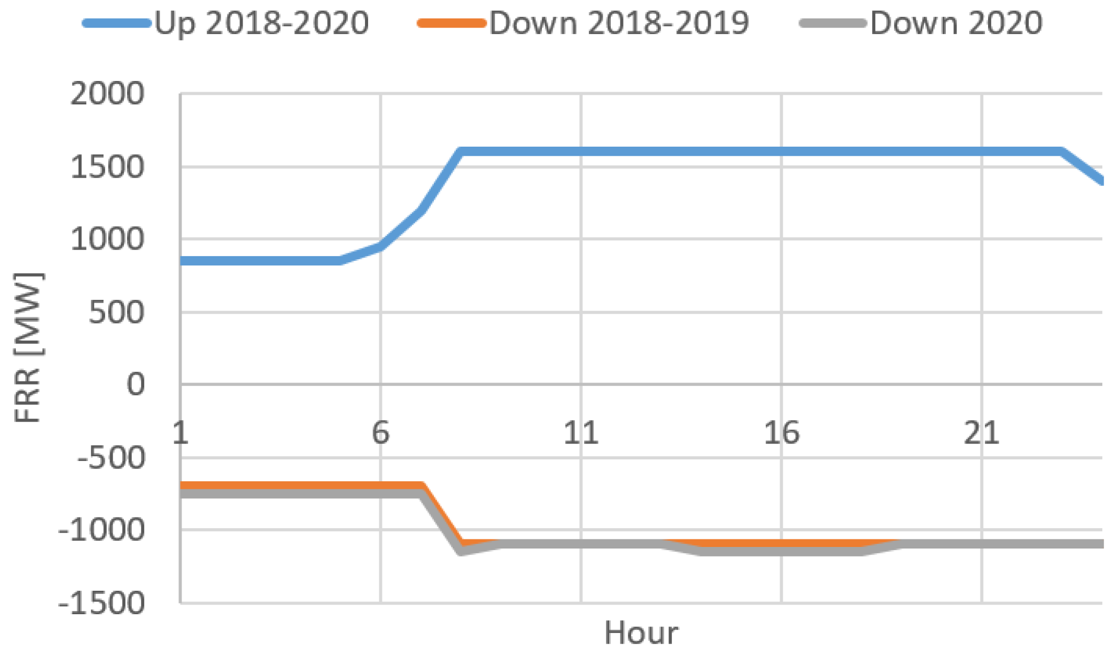
  • The upward capacity requirement of Figure 1 served all but 4/99,360 incidents, as noted in Section 3.5.
  • The downward capacity requirement of Figure 1 served all but 30/99,360 incidents, as noted in Section 3.5.
The results are presented in Table 2. A number of effects that are consistent with intuition can be observed: (i) Downward reserve requirements are lower than upward reserve requirements for a given day type, due to the asymmetric risk of contingencies in upward requirements. (ii) Higher load implies higher reserve requirements. (iii) Higher renewable supply implies higher reserve requirements. (iv) Higher imports imply higher reserve requirements. (v) The effect of load on reserve requirements is the strongest; the effect of imports on reserve requirements is the least strong.

5. Case Study of Probabilistic Dimensioning

This section compares the dimensioning of Figure 1 to the probabilistic dimensioning method based on k-means.

5.1. Case Study Description

As indicated previously in the article, system imbalance data have not been made available for this study. Instead, we employed other data that are publicly available at the websites of the Greek market operator and the Greek transmission system operator, and data provided by the Greek regulatory authority for energy, in order to calibrate a model of system imbalances which captures salient system characteristics, as indicated in Section 3. The specific input data used for the analysis are briefly recalled below.
Reserve requirement data for the Greek system for 2018–2020 were sourced from the following link of the Hellenic Energy Exchange, which was accessed on 20 August 2021: https://www.enexgroup.gr/el/day-ahead-scheduling-archive. In addition to reserve requirement data, the website includes the day-ahead schedules of individual units, and a number of other scheduling results related to dispatch and reserve provision.
Additionally, the following data have been provided by the Regulatory Authority for Energy:
  • Load data with hourly resolution from 1 January 2018 until 31 October 2020, thus spanning 2 years and 10 months (namely, 1035 days).
  • Renewable energy supply data with the same characteristics.
  • Import/export data with the same characteristics.
The results are presented in Table 3 and Table 4. For each sizing policy, the following metrics are reported for both the upward and downward direction in Table 3:
  • Average reserves committed, measured in MW.
  • Unreliability: a measure of how many incidents of oversupply or undersupply occur per year, measured in hours per year. This corresponds to the loss of load expectation (LOLE) measure in reliability studies, but is here measured in both the case of upward and downward imbalances.
  • Shortage or oversupply, measured in MWh/year. This corresponds to expected energy not served in adequacy studies, but is also measured in the downward direction (in the sense of quantity of energy oversupplied).
Moreover, Table 4 reports the relative contribution of each day type to the overall failure profile of each reserve sizing policy. This is explained further in Section 5.3.

5.2. Reserve Requirements

With respect to the reserves committed by the compared sizing methods, one can observe that the probabilistic dimensioning approach achieved a significant improvement in the upward dimensioning requirement, with average upward reserves being reduced by 281 MW, or 20.2% of the average upward requirement of Figure 1. Similarly, the downward dimensioning decreased by 43 MW, or 4.3%, which is less than the savings of the upward dimensioning, but still notable.
In terms of reliability performance, it can be observed that the sizing of Figure 1 remained close to the failure target of 3 h/year. The probabilistic dimensioning resulted in total failures of 2.3 h/year, thereby staying below the reliability target of 3 h/year. The MWh of shortage and oversupply were correspondingly lower values in the case of the probabilistic dimensioning method. Thus, the probabilistic dimensioning method was more reliable, while also relying on less reserves.
The results presented in Table 3 are based on an out-of-sample simulation, in the sense that an entirely new sample of 99,360 imbalance intervals (2 years and 10 months) was generated, based on the imbalance driver data that were provided by the regulatory authority, and based on the imbalance model that was developed in Section 3.

5.3. Risk Profile

Table 4 presents the numbers of intervals that belong to the clusters of the probabilistic dimensioning method. These are equal in both the training and the testing phase, since the same day-ahead data were used for both training and testing. The table additionally presents the number of failures that occurred in each day type in the testing phase, for both the sizing of Figure 1 and the probabilistic dimensioning. This serves as a measure of the risk assumed by each of the methods.
An indication of the extent to which a sizing method is able to maintain a constant level of risk is how well the observed out-of-sample risk of the method is able to track the frequency of each interval type. This assessment is shown in Figure 3. The horizontal axis of the figure represents the eight day types/clusters that were considered in the analysis. The blue curve corresponds to the empirical frequencies of occurrence of the eight day types in the out-of-sample simulation. For instance, for day type “HHH” (the first day type), the blue curve demonstrates that it occurred 13.4% of the time. The orange curve then depicts the relative contributions of failures in these day types to the total failures for the probabilistic sizing method. For day type “HHH”, reading off of the orange curve implies that failures in this day type contributed to 18.5% of the total failures of the probabilistic sizing method. Similarly, the gray curve provides the corresponding figure for the sizing method of Figure 1. Reading again off of the figure for day type “HHH”, it can be observed that failures in this day type correspond to 14.3% of the total failures of this reserve sizing method.
One can observe in Table 4 that, although interval type 7 (low load, low renewable supply, large amount imported) corresponds to 26.5% of the intervals in the data sample, the sizing method of Figure 1 exhibits a frequency of failures in the seventh interval type, which is twice as high as the frequency of this interval type. This indicates that a fixed reserve requirement corresponding to Figure 1 tends to be undersized for this specific interval type (which corresponds to a quarter of the time).
Figure 3 represents the percentages of Table 3 visually. The closer the curves remain to the blue curve, the more consistent they are in terms of maintaining a constant risk. Deviating too far above the blue curve indicates an exposure to a disproportionately high risk (i.e., undersizing), and deviating too far below the blue curve indicates an exposure to a disproportionately low risk (i.e., oversizing). It is clear that the probabilistic dimensioning method was able to remain closer to the blue curve, thereby indicating an improved risk profile relative to the sizing of Figure 1. Similar results emerged with the probabilistic dimensioning method that was employed in Belgium [2].

5.4. Integration with System Operations

An alternative way to approach the simulation could be to implement it in a rolling fashion, in the sense of training a sizing model once a year, based on the data of the past year. One would then use the trained clustering algorithm one day in advance of operations in order to determine the cluster in which the following day belongs, so as to then decide on the reserve capacity that should be procured for the day ahead. This is the approach that has been proposed and considered for implementation in the Belgian system [2]. The timeline of this rolling procedure is depicted in Figure 4, which is similar in spirit to [2].
The figure outlines a rolling procedure, where training takes place once a year, six months in advance of the beginning of the relevant year of operation. The clustering of days into day types takes place in the “k-means clustering” box. These clusters are then used for deriving reserve requirements for different day types according to probabilistic criteria in the “Probabilistic reserve sizing” box. This allows the system operator to have at hand a mapping of day types to upward and downward reserve requirements. On the day ahead of operation (indicated in the figure as the gray “Day ahead” box), the system operator can identify the day type that is anticipated for the following day based on the observable day-ahead explanatory factors (renewable supply forecasts, load forecasts, and import forecasts in the case of the present publication). Once the day type of the coming day is identified, the pre-computed mapping of the day type to the corresponding probability distribution and thus the appropriate quantile which implies the reserve requirement for the following day can be determined. The sizing result can then be used as input for the day-ahead procurement of reserve capacity, which may take place before, simultaneously with, or after the day-ahead procurement of energy. The Greek market specifically operates an integrated scheduling process (ISP), where reserves are committed on a daily basis (with three runs of ISP, on the day ahead and two intraday adjustment runs). The proposed probabilistic dimensioning procedure would then generate input for this ISP procedure.
An important attribute of this process relates to regulatory approval. Reserve requirements proposed by the TSO are typically approved by the competent national regulatory authority on an annual basis. Since reserve requirements vary on a daily basis according to the above procedure, what would be required in the proposed implementation would be the regulatory approval of the proposed methodology, instead of the MW requirement itself [2].
Note that the procedure described above and investigated in this paper can be improved in a number of ways. The analysis would clearly benefit from the presence of real system imbalance data. The levels of detail of the analysis could have been improved by considering the generator availability of each day of the year, instead of the eight days indicated in Section 3.2. Alternative probabilistic methods are also worth considering in future work, with common alternatives considered in the literature including k-nearest neighbors clustering [2] and quantile regression based on artificial neural networks [28], although the latter has been found to perform poorly in small systems where contingencies dominate sizing decisions. An crucial extension from a practical standpoint is the careful analysis of various alternatives for joint dimensioning of aFRR and mFRR capacity, and the consideration of transmission constraints which pertain to reserve deliverability [42]. The author is currently working on those two extensions, and preliminary results have been presented in [43].

6. Conclusions

Probabilistic dimensioning is becoming increasingly relevant in European systems, due to the spirit of EU law—in particular, the System Operation Guideline [10] and the Electricity Balancing Guideline [44]—which places loss of load probability as the cornerstone criterion of reserve sizing. This paper specifically considered the reserve dimensioning method that is advancing towards implementation in the Belgian electricity market, and examined its possible application in the Greek electricity system.
The initial investigation presented in this paper suggests that probabilistic dimensioning may merit further investigation for the Greek electricity system. Significant potential savings were uncovered in the sizing of upward frequency restoration capacity, and notable savings in the sizing of downward balancing capacity. These savings resulted from the fact that the system can adapt its sizing to the anticipated day type: days with higher risk can be planned with more reserves at hand, but days with lower risk can be planned with less reserves, with the end result being that the average reserves are reduced throughout the year. The adaptive nature of the sizing of the reserve requirement also allows the system to operate at a more constant level of risk. This should be contrasted with a static sizing method, where days with less favorable conditions expose the system to greater risk, and during days with more favorable conditions the system is over-protected and carries unnecessarily high reserves.
In order to conduct the analysis, and in the absence of system imbalance data, the paper proposed a stochastic model of imbalances which captures a number of salient features which render dynamic dimensioning relevant. These features include skewed distributions, the dependencies of the imbalance distribution on the levels of various imbalance drivers, and the contribution of idiosyncratic noise to system imbalances.
Additionally, the literature review provides a lookup table that can be useful for practitioners navigating among the range of options that can be considered for implementation in system operations. The classification of the literature was performed using three axes, including the analytical method that can be used for dimensioning (heuristics, probabilistic dimensioning, or bottom-up models), static versus dynamic dimensioning, and whether the proposed method relies on a parametric or non-parametric model of uncertainty.
The procedure described in the paper can be improved in a number of way. An extension that is crucial from a practical standpoint is the application of probabilistic dimensioning to the joint dimensioning of aFRR and mFRR capacity, which goes beyond the current state of the art [11,12,13,15,29,34,38]. Transmission constraints which pertain to reserve deliverability will also need to be considered [42].

Funding

This research has been supported by the Hellenic Regulatory Authority for Energy.

Institutional Review Board Statement

Not applicable.

Informed Consent Statement

Not applicable.

Conflicts of Interest

The author declare no conflict of interest.

References

  1. Papavasiliou, A.; Oren, S.S.; O’Neill, R.P. Reserve requirements for wind power integration: A scenario-based stochastic programming framework. IEEE Trans. Power Syst. 2011, 26, 2197–2206. [Google Scholar] [CrossRef] [Green Version]
  2. De-Vos, K.; Stevens, N.; Devolder, O.; Papavasiliou, A.; Hebb, B.; Matthys-Donnadieu, J. Dynamic Dimensioning Approach for Operating Reserves: Proof of Concept in Belgium. Energy Policy 2019, 124, 272–285. [Google Scholar] [CrossRef]
  3. ENTSO-E. Load-Frequency Control and Performance. In Continental Europe Operation Handbook; Technical Report; ENTSO-E: Brussels, Belgium, 2009. [Google Scholar]
  4. Holttinen, H.; Milligan, M.; Kirby, B.; Acker, T.; Neimane, V.; Molinski, T. Using standard deviation as a measure of increased operational reserve requirement for wind power. Wind Eng. 2008, 32, 355–377. [Google Scholar] [CrossRef]
  5. Ohsenbruegge, A.; Klingenberg, T.; Lehnhoff, S. Dynamic Data Driven Dimensioning of Balancing Power with k-Nearest Neighbors. In Proceedings of the Power and Energy Student Summit (PESS) 2015, Dortmund, Germany, 13–14 January 2015. [Google Scholar]
  6. Ohsenbrugge, A.; Lehnhoff, S. Dynamic Dimensioning of Balancing Power with Flexible Feature Selection. In Proceedings of the 23rd International Conference on Electricity Distribution, Lyon, France, 15–18 June 2015. [Google Scholar]
  7. Dvorkin, Y.; Ortega-Vazuqez, M.A.; Kirschen, D.S. Wind generation as a reserve provider. IET Gener. Transm. Distrib. 2015, 9, 779–787. [Google Scholar] [CrossRef] [Green Version]
  8. Papavasiliou, A.; Oren, S.S. Multi-Area Stochastic Unit Commitment for High Wind Penetration in a Transmission Constrained Network. Oper. Res. 2013, 61, 578–592. [Google Scholar] [CrossRef]
  9. European Commission. Commission Regulation (EU) 2017/2195 of 23 November 2017 Establishing a Guideline on Electricity Balancing; Technical Report; European Commission: Brussels, Belgium, 2017. [Google Scholar]
  10. European Commission. Commission Regulation (EU) 2017/1485 of 2 August 2017 Establishing a Guideline on Electricity Transmission System Operation; Technical Report; European Commission: Brussels, Belgium, 2017. [Google Scholar]
  11. Jost, D.; Speckmann, M.; Sandau, F.; Schwinn, R. A new method for day-ahead sizing of control reserve in Germany under a 100% renewable energy sources scenario. Electr. Power Syst. Res. 2015, 119, 485–491. [Google Scholar] [CrossRef]
  12. Breuer, C.; Engelhardt, C.; Moser, A. Expectation-based reserve capacity dimensioning in power systems with an increasing intermittent feed-in. In Proceedings of the 2013 10th International Conference on the European Energy Market (EEM), Stockholm, Sweden, 27–31 May 2013. [Google Scholar]
  13. Maurer, C.; Krahl, S.; Weber, H. Dimensioning of secondary and tertiary control reserve by probabilistic methods. Eur. Trans. Electr. Power 2009, 19, 544–552. [Google Scholar] [CrossRef]
  14. Kays, J.; Schwippe, J.; Rehtanz, C. Dimensioning of reserve capacity by means of a multidimensional method considering uncertainties. In Proceedings of the IEEE PSCC Stockholm Conference, Stockholm, Sweden, 22–26 August 2011. [Google Scholar]
  15. Kippelt, S.; Schlüter, T.; Rehtanz, C. Flexible dimensioning of control reserve for future energy scenarios. In Proceedings of the 2013 IEEE Grenoble Conference, Grenoble, France, 16–20 June 2013. [Google Scholar]
  16. Dvorkin, Y.; Pandžić, H.; Ortega-Vazquez, M.A.; Kirschen, D.S. A hybrid stochastic/interval approach to transmission-constrained unit commitment. IEEE Trans. Power Syst. 2014, 30, 621–631. [Google Scholar] [CrossRef]
  17. Meibom, P.; Barth, R.; Hasche, B.; Brand, H.; Weber, C.; O’Malley, M. Stochastic optimization model to study the operational impacts of high wind penetrations in Ireland. IEEE Trans. Power Syst. 2010, 26, 1367–1379. [Google Scholar] [CrossRef]
  18. Dietrich, K.; Latorre, J.; Olmos, L.; Ramos, A.; Perez-Arriaga, I. Stochastic unit commitment considering uncertain wind production in an isolated system. In Proceedings of the 4th Conference on Energy Economics and Technology, Dresden, Germany, 3–6 April 2009. [Google Scholar]
  19. Bertsimas, D.; Litvinov, E.; Sun, X.A.; Zhao, J.; Zheng, T. Adaptive Robust Optimization for the Security Constrained Unit Commitment Problem. IEEE Trans. Power Syst. 2013, 28, 52–63. [Google Scholar] [CrossRef]
  20. Ortega-Vazquez, M.A.; Kirschen, D.S. Estimating the spinning reserve requirements in systems with significant wind power generation penetration. IEEE Trans. Power Syst. 2008, 24, 114–124. [Google Scholar] [CrossRef]
  21. Zhou, Z.; Botterud, A.; Wang, J.; Bessa, R.J.; Keko, H.; Sumaili, J.; Miranda, V. Application of probabilistic wind power forecasting in electricity markets. Wind Energy 2013, 16, 321–338. [Google Scholar] [CrossRef]
  22. Tuohy, A.; Meibom, P.; Denny, E.; O’Malley, M. Unit Commitment for Systems with High Wind Penetration. IEEE Trans. Power Syst. 2009, 24, 592–601. [Google Scholar] [CrossRef] [Green Version]
  23. Gooi, H.; Mendes, D.; Bell, K.; Kirschen, D. Optimal scheduling of spinning reserve. IEEE Trans. Power Syst. 1999, 14, 1485–1492. [Google Scholar] [CrossRef]
  24. Bessa, R.J.; Mendes, J.; Miranda, V.; Botterud, A.; Wang, J.; Zhou, Z. Quantile-copula density forecast for wind power uncertainty modeling. In Proceedings of the 2011 IEEE Trondheim PowerTech, Trondheim, Norway, 19–23 June 2011. [Google Scholar]
  25. Bessa, R.J.; Miranda, V.; Botterud, A.; Zhou, Z.; Wang, J. Time-adaptive quantile-copula for wind power probabilistic forecasting. Renew. Energy 2012, 40, 29–39. [Google Scholar] [CrossRef]
  26. Bruninx, K.; Delarue, E. A statistical description of the error on wind power forecasts for probabilistic reserve sizing. IEEE Trans. Sustain. Energy 2014, 5, 995–1002. [Google Scholar] [CrossRef]
  27. Elia. Evolution of Ancillary Services Needs to Balance the Belgian Control Area towards 2018; Technical Report; Elia: Brussels, Belgium, 2013. [Google Scholar]
  28. Jost, D.; Braun, A.; Fritz, R. Dynamic Dimensioning of Frequency Restoration Reserve Capacity based on Quantile Regression. In Proceedings of the 12th International Conference on the European Energy Market (EEM), Lisbon, Portugal, 19–22 May 2015. [Google Scholar]
  29. Jost, D.; Braun, A.; Fritz, R.; Otterson, S. Dynamic sizing of automatic and manual frequency restoration reserves for different product lengths. In Proceedings of the 2016 13th International Conference on the European Energy Market (EEM), Porto, Portugal, 6–9 June 2016. [Google Scholar]
  30. Juban, J.; Siebert, N.; Kariniotakis, G.N. Probabilistic short-term wind power forecasting for the optimal management of wind generation. In Proceedings of the 2007 IEEE Lausanne Power Tech, Lausanne, Switzerland, 1–5 July 2007; pp. 683–688. [Google Scholar]
  31. Kim, S.K.; Park, J.H.; Yoon, Y.T. Determination of Secondary Reserve Requirement Through Interaction-dependent Clearance Between Ex-ante and Ex-post. J. Electr. Eng. Technol. 2014, 9, 71–79. [Google Scholar] [CrossRef]
  32. Menemenlis, N.; Huneault, M.; Robitaille, A. Computation of dynamic operating balancing reserve for wind power integration for the time-horizon 1–48 h. IEEE Trans. Sustain. Energy 2012, 3, 692–702. [Google Scholar] [CrossRef]
  33. Nielsen, H.A.; Madsen, H.; Nielsen, T.S. Using quantile regression to extend an existing wind power forecasting system with probabilistic forecasts. Wind Energy 2006, 9, 95–108. [Google Scholar] [CrossRef]
  34. De Vos, K.; Morbee, J.; Driesen, J.; Belmans, R. Impact of wind power on sizing and allocation of reserve requirements. IET Renew. Power Gener. 2013, 7, 1–9. [Google Scholar] [CrossRef]
  35. Zhou, Z.; Botterud, A. Dynamic Scheduling of Operating Reserves in Co-Optimized Electricity Markets with Wind Power. IEEE Trans. Power Syst. 2014, 29, 160–171. [Google Scholar] [CrossRef]
  36. Zhang, Y.; Wang, J.; Wang, X. Review on probabilistic forecasting of wind power generation. Renew. Sustain. Energy Rev. 2014, 32, 255–270. [Google Scholar] [CrossRef]
  37. Ren, Z.; Yan, W.; Zhao, X.; Li, W.; Yu, J. Chronological Probability Model of Photovoltaic Generation. IEEE Trans. Power Syst. 2014, 29, 1077–1088. [Google Scholar] [CrossRef]
  38. Bucksteeg, M.; Niesen, L.; Weber, C. Impacts of Dynamic Probabilistic Reserve Sizing Techniques on Reserve Requirements and System Costs. IEEE Trans. Sustain. Energy 2016, 7, 1408–1420. [Google Scholar] [CrossRef]
  39. ADMIE. Methodology for the Determination of Zonal/System Needs for Balancing Power; Technical Report; ADMIE: Athina, Greece, 2020. [Google Scholar]
  40. Lloyd, S. Least squares quantization in PCM. IEEE Trans. Inf. Theory 1982, 28, 129–137. [Google Scholar] [CrossRef]
  41. Arthur, D.; Vassilvitskii, S. k-Means++: The Advantages of Careful Seeding; Technical Report; Stanford InfoLab Publication Server: Stanford, UK, 2006. [Google Scholar]
  42. Zheng, T.; Litvinov, E. Contingency-based zonal reserve modeling and pricing in a co-optimized energy and reserve market. IEEE Trans. Power Syst. 2008, 23, 277–286. [Google Scholar] [CrossRef]
  43. Papavasiliou, A.; Bouso, A.; Apelfröjd, S.; Wik, E.; Gueuning, T.; Langer, Y. Multi-Area Reserve Dimensioning Using Chance-Constrained Optimization; Technical Report; IEEE: Piscataway, NJ, USA, 2021. [Google Scholar]
  44. European Commission. EU Reference Scenario 2016; Technical Report; European Commission: Brussels, Belgium, 2016. [Google Scholar]
Figure 1. Representative reserve sizing values for upward/downward capacity in the Greek electricity market in 2018–2020.
Energies 14 05719 g001
Figure 2. Left panel: Hypothetical probability distribution function of renewable supply (RES-driven imbalance plus the underlying imbalance driver) which exceeds installed RES capacity. Right panel: Probability distribution function of renewable supply which reflects on the installed capacity boundary.
Energies 14 05719 g002
Figure 3. Frequency of each interval type, and frequency of failures for the probabilistic dimensioning method and the sizing of Figure 1.
Energies 14 05719 g003
Figure 4. Timeline of a probabilistic dimensioning procedure, where the training of the probabilistic dimensioning algorithm takes place once a year based on the data of the previous year.
Energies 14 05719 g004
Table 1. A classification of reserve sizing literature.
HeuristicProbabilisticUC/EDStaticDynamicParametric pdfsNon-Parametric pdfs
 [24] X
 [25] X
 [19] X X
 [26] XX
 [12] X X
 [18] XX
 [16] X X
 [7]X X X
 [3]X X
 [27] X X
 [23] XXX X
 [4]X X
 [28] X X
 [11] X X X
 [29] X X X
 [30] X
 [15] X X
 [14] X X X
 [31]X XX
 [32] X XX
 [13] X XX
 [17] X X
 [33] X
 [20]X X XX
 [5]X X
 [6]X X
 [1] X X
 [22] X X
 [34] X X
[2] X X X
 [35] X X
 [36] XX
 [21] X X X
 [37] X
Table 2. Reserve requirement for each type of day. All quantities are in MW.
LoadRenewablesImportsReserve UpReserve Down
6810 (H)2091 (H)1331 (H)13831085
6810 (H)2091 (H)471 (L)12821043
6810 (H)782 (L)1331 (H)11191028
6810 (H)782 (L)471 (L)1187919
4886 (L)2091 (H)1331 (H)981855
4886 (L)2091 (H)471 (L)912845
4886 (L)782 (L)1331 (H)991802
4886 (L)782 (L)471 (L)970737
Table 3. Comparative results of the probabilistic dimensioning against the sizing of Figure 1.
Figure 1Probabilistic
Res-Up (MW)13921111
Unrel.-Up (hours/y)0.30.4
Shortage (MWh/y)40.221.5
Res-Down (MW)993950
Unrel.-Down (hours/y)2.81.9
Oversupply (MWh/y)208.4159.1
Table 4. Number of intervals belonging to each cluster of the probabilistic dimensioning method and corresponding number of incidents within each cluster.
Interval TypeNo. OccurrencesFails Prob. (h/yr)Fails Figure 1 (h/yr)
LoH-ReH-ImH13,292 (13.4%)0.44 (18.5%)0.44 (14.3%)
LoH-ReH-ImL9644 (9.7%)0.09 (3.7%)0.09 (2.9%)
LoH-ReL-ImH12,144 (12.2%)0.09 (3.7%)0.26 (8.6%)
LoH-ReL-ImL10,812 (10.9%)0.53 (22.2%)0.09 (2.9%)
LoL-ReH-ImH7960 (8.0%)0.26 (11.1%)0.18 (5.7%)
LoL-ReH-ImL6952 (7.0%)0.09 (3.7%)0.09 (2.9%)
LoL-ReL-ImH26,296 (26.5%)0.53 (22.2%)1.59 (51.4%)
LoL-ReL-ImL12,260 (12.3%)0.35 (14.8%)0.35 (11.4%)
Publisher’s Note: MDPI stays neutral with regard to jurisdictional claims in published maps and institutional affiliations.

