Article

Generation Expansion Planning with Energy Storage Systems Considering Renewable Energy Generation Profiles and Full-Year Hourly Power Balance Constraints

by
Radhanon Diewvilai
1 and
Kulyos Audomvongseree
1,2,*
1
Department of Electrical Engineering, Chulalongkorn University, Bangkok 10330, Thailand
2
Energy Research Institute, Chulalongkorn University, Bangkok 10330, Thailand
*
Author to whom correspondence should be addressed.
Energies 2021, 14(18), 5733; https://doi.org/10.3390/en14185733
Submission received: 29 July 2021 / Revised: 2 September 2021 / Accepted: 9 September 2021 / Published: 11 September 2021
(This article belongs to the Special Issue Power System Planning and Quality Control)

Abstract

:
This paper proposes a methodology to develop generation expansion plans considering energy storage systems (ESSs), individual generation unit characteristics, and full-year hourly power balance constraints. Generation expansion planning (GEP) is a complex optimization problem. To get a realistic plan with the lowest cost, acceptable system reliability, and satisfactory CO2 emissions for the coming decades, a complex multi-period mixed integer linear programming (MILP) model needs to be formulated and solved with individual unit characteristics along with hourly power balance constraints. This problem requires huge computational effort since there are thousands of possible scenarios with millions of variables in a single calculation. However, in this paper, instead of finding the globally optimal solutions of such MILPs directly, a simplification process is proposed, breaking it down into multiple LP subproblems, which are easier to solve. In each subproblem, constraints relating to renewable energy generation profiles, charge-discharge patterns of ESSs, and system reliability can be included. The proposed process is tested against Thailand’s power development plan. The obtained solution is almost identical to that of the actual plan, but with less computational effort. The impacts of uncertainties as well as ESSs on GEP, e.g., system reliability, electricity cost, and CO2 emission, are also discussed.

1. Introduction

1.1. Motivation

Long-term generation expansion planning (GEP) is one of the most complicated problems relating to electrical power generation systems. A growing population, economic development, and electrification are major causes of increasing electricity demand [1], and electrical power systems need to be expanded to meet this forecasted energy consumption. To ensure the availability and reliability of the system with acceptable cost for electricity, new generation units must be carefully selected and developed in advance. This requires a decision-making process to determine which generation units using different technology, fuel types, sizes, operational characteristics, etc., should be commissioned into the system at specific locations and times within the stages of the planning horizon [2,3]. Thus, complex optimization models have been developed to take economic, technical, environmental, and other pertinent constraints into consideration during long-term generation expansion planning.
Renewable energy penetration, especially variable renewable energy (VRE) such as wind and solar power, is a major concern for both generation expansion and operation planning. The integration of variable renewable energy into the electricity grid may lead to the emergence of other crucial considerations, such as the reliability and flexibility of the power system [3]. To deal with the intermittency caused by these VRE generators, energy storage systems (ESSs) have been introduced [4]. Since both renewable energy and energy storage systems will play even more important roles in power systems in the near future, it is necessary for the generation expansion planning model to incorporate both items and provide a generation expansion plan with adequate generation capacity for the power system. Furthermore, a full-year, 8760-hour resolution model with hourly load balance constraints should also be required so that the intermittent characteristics of renewable energy sources, which vary by time of day and season, can be taken into account.

1.2. Literature Review

There are many optimization techniques proposed to solve long-term generation expansion planning problems. They include linear programming (LP) [5], integer programming (IP) [6,7,8], non-linear programming (NLP) [9,10,11], dynamic programming (DP) [3,12,13], and metaheuristic method [14,15,16]. Although the complete optimization technique for long-term generation expansion planning is large-scale, highly constrained mixed-integer non-linear programming (MINLP) [7] with multiple decision criteria, uncertainties, and a dynamic nature [17], simplified models like mixed-integer linear programming (MILP) are widely used to avoid the considerable computational complexity associated with such non-linear methods or search algorithms [7]. Since an actual generation expansion planning horizon is a long-period of time, 15 to 20 years or even longer as shown in [18,19], a multi-year planning model that considers several stages of generation capacity may offer more supportive information for decision-making compared to a target-year model [20]. Thus, several models, so-called multi-period MILP, have been developed for long-term generation expansion planning. The objective function of this optimization problem is usually total electricity cost minimization, which might include environmental impact mitigation costs. Constraints of the problem comprise supply–demand balance constraints, system reliability constraints, environmental constraints, energy mixing constraints, fuel limitation constraints, etc. To solve this optimization problem, for example, Koltsaklis et al. proposed a multi-period MILP model with area discretization and integrated energy resource management [7]; Afful-Dadzie et al. proposed a multi-period stochastic MILP with budget constraints [21]; Guerra et al. proposed multi-period MILP model for generation and transmission expansion planning [22]; and Koltsaklis et al. proposed a multi-period MILP model with operation constraints [23].
To create a more realistic model, each power generation unit needs to be considered individually. By doing this, each individual unit characteristics and parameters such as heat rate, fuel cost, and emission rate can be taken into account in the calculation [24]. A full-year, 8760-hour resolution model with hourly load balance constraints is also required in order to account for the intermittent characteristics of renewable energy sources [25], which vary by time of day and season. However, with these constraints, generation expansion planning problems formulated using MILP are too complex to be solved for a time horizon of an entire year [25]. To reduce the large number of variables that need to be considered, traditional generation expansion planning models do not attempt to consider all hours consecutively within a year, but rather analyze only a limited number of temporally independent slices [26]. For example, Koltsaklis et al. consider hourly load balance and unit commitment constraints only for a representative day of each month in the planning horizon [23]. Alternatively, neglecting timely power balance constraints, Koltsaklis et al. and Afful-Dadzie et al. [7,21] represent demand in each time period with total annual demand, while Guerra et al. use separated annual demand of each area as representative. Such simplifications could lead to over optimistic scenarios for renewable energy source penetration [26], since either the hourly or seasonally intermittent characteristics of renewable energy sources are neglected. Moreover, the use of representative day is not detailed enough if there is ESS in the system since ESS might not be necessary to be fully charged and discharged within a day. Additionally, with representative day model, several constraints are also ignored, e.g., annual fuel-mix constraint due to lack of annual energy demand information. Additionally, it neglects seasonal or holiday load characteristic. To cope with aforementioned flaws, many researches introduce multiple representative days concept [23,27]. Therefore, both individual unit characteristics and full-year hourly load balance constraints with renewable energy generation profiles are required to avoid over-simplification in the model.
Considering actual national level generation expansion planning problems, the multi-period MILP model with hourly power balance constraints is a large and complicated model since the system consists of hundreds to thousands of large-scale power plants, as in the generation system in Thailand [17]. Moreover, with a 20-year planning horizon and multiple options for generation expansion decisions, millions of variables need to be analyzed simultaneously. Thus, this problem would require huge computational time and effort. There are scholars who have also proposed MILP models with individual unit characteristics along with hourly power balance constraints. Belderbos et al. proposed an integrated model of system planning and short-term operational model in [25] and Chen et al. proposed a two-level model (capacity expansion and operational) in [26]. However, both are target-year models, which do not provide appropriate commissioning time for each new generation capacity. Belderbos’s model also lacks some important constraints, i.e., greenhouse gas emissions and energy-mix constraints, while Chen’s model requires high computational effort to solve, since even an annual simulation involves approximately 2.3 million variables.
There are several non-linear generation reliability indices being considered in generation expansion planning, e.g., LOLE or LOLP [28], which are reliability indexes calculated from the Capacity Outage Probability Table (COPT) [28] created from all generation units and their Forced Outage Rate (FOR), and Load Duration Curve (LDC). LOLE has been considered in several publications since both generation system and load pattern are considered, unlike reserve margin, which considers only total installed capacity and peak load. However, most of them use an estimated value of LOLE instead of the actual one. For example, Aghaei et al. model LOLE constraint using the corresponding Z constraint from the Z-Method [29]; Pudjiato et al. use a piecewise linear function to approximate the LOLP function in the MILP model [30]; and Opathella et al. approximate LOLP based on the linear LOLP variation within the MILP model [27]. However, use of the estimated value might lead to errors in calculation due to the non-linear characteristic of the index.
Recently, Energy Storage Systems (ESSs) have been included in analyses in many publications relating to generation expansion planning or economic dispatch since ESSs are widely accepted as effective tools to mitigate the impacts of variable renewable energy on power system operation and planning. For example, Opathella et al. propose an MILP formulation for generation and storage expansion planning with power balance constraints [27]; Hemmati et al. propose a two-level microgrid planning tool considering distributed generation resources and ESSs [31]; Choi et al. present economic dispatch of the grid-connected microgrid with multiple ESSs [32]; Xiong and Singh propose an approach for determining the optimal location and size of ESSs in power systems with wind power generation in which economic dispatch and load flow need to be solved [33]. In this paper, 2 types of ESS, Pumped Hydro Storage (PHS) and Battery Energy Storage Systems (BESS), and their specific parameters are incorporated into the economic dispatch problem as well as into LOLE calculation.

1.3. Our Contribution

This paper proposes a simplified multi-period linear programming model for generation expansion planning (GEP). Instead of solving for a global optimum using the complex model, the total planning time horizon, e.g., 20 years, is divided into multiple periods, e.g., 240 months, to reduce the size of the subproblem in each calculation. A decision-making process to determine whether a new generation unit should be added to the generation system is also separated from the optimization model in order to get rid of integer variables. At each consideration period, a generation unit with appropriate fuel type can be added into the system only if reliability indices, e.g., reserve margin capacity or Loss of Load Expectation (LOLE), or other constraints, such as fuel mix and CO2 emissions, of the system have not met acceptable criteria. Therefore, the large-scale multi-period MILP problem can be decomposed into multiple linear programming subproblems. With these separated and simplified models, solutions to the subproblems associated with each period can be easily obtained. Solution for earlier period that satisfy all criteria will then be used as the initial conditions for the subproblem of the next period. With these smaller scale subproblems, hourly power balance constraints with renewable energy generation profiles for a whole subperiod, e.g., 720 h in a month, can be included in the model without too much computational burden. The process will then be repeated from the first until the last period, covering the total planning time horizon. Another benefit of the separation of this decision-making process and optimization model is the ability to incorporate non-linear power system indices calculation. The proposed separation process allows non-linear indices, i.e., LOLE, to be calculated during the decision-making process, instead of being estimated as they are in other optimization models.
With this simplified model, unit commitment and energy dispatch problems with variable renewable energy (VRE) and energy storage systems (ESSs) can be solved along with other non-linear indices. Furthermore, LOLE calculation considering energy storage systems is also proposed in this paper. Although this simplification technique does not guarantee global optimal solution, from the case study, we found that it is still an efficient method as computational effort is greatly reduced while the obtained solution is still close to the original plan. The novelty of this work is that it is a multi-year GEP model considering individual unit characteristics, both generation capacity and ESSs, along with hourly power balance constraints for every month within the planning horizon. Furthermore, since the computational time is greatly reduced, uncertainty of input data can be considered by solving multiple GEP problems with variable input data and different individual probability. The proposed method is tested with Thailand’s power generation system with input data and assumptions from Thailand’s Power Development Plan published in 2012 (PDP2010 rev.3) [19]. The result from the proposed method is then compared with that of the PDP2010 rev.3 to confirm its accuracy.
The rest of this manuscript is organized as follows: Section 2 presents the problem statement and mathematical formulation of the proposed model. Section 3 describes the case study, Thailand’s Power Development Plan 2010 revision 3, used to test the proposed model. Section 4 discusses the results of the case study. Finally, a concluding remark is given and directions for future work are discussed.

2. Methodology

2.1. Problem Statement

This paper addresses the long-term national level generation expansion planning problem of a centralized power generation system. The problem in this study is defined in the terms of the following factors and assumptions:
  • The model is deterministic.
  • Adequacy of generation capacity can be ensured by exceeded capacity results from reliability constraints.
  • The objective of this problem is to create a generation expansion plan that has minimum total electricity cost. Total electricity cost consists of average and levelized investment costs, fuel costs, fixed operation and maintenance costs, and variable operation and maintenance costs.
  • The given planning horizon is divided into monthly timeslots.
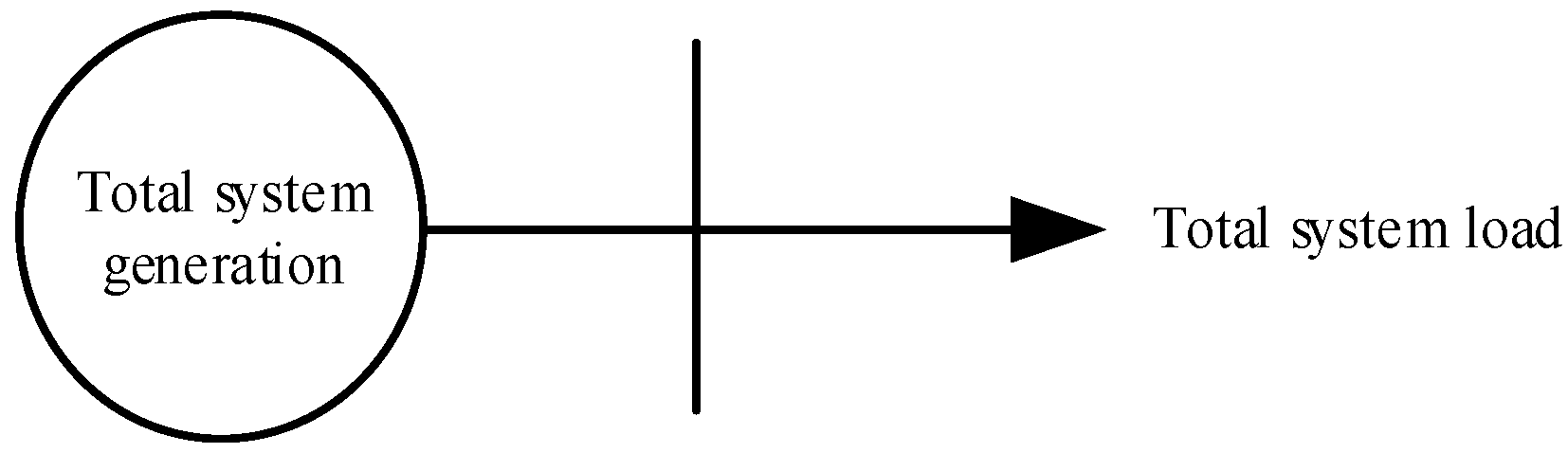
  • The power system is modelled as a conventional system as shown in Figure 1. Only generation and total system load are considered. Transmission elements are neglected.
  • The initial generation system prior to the given planning horizon is required.
  • Renewable energy penetration is already planned for a whole planning horizon.
  • A set of candidate units for generation expansion are given with different technologies, fuels, sizes, and heat rates.
  • Operational and short-term characteristics, e.g., ramp rates, minimum up and down times, synchronization and desynchronization time, etc., are neglected in this optimization.
  • Only generation system reliability is considered. Transmission system reliability is neglected.
  • The individual hourly output power of each generation unit is considered to accurately represent power generation profile of intermittent renewable energy resources. For example, non-dispatchable solar generation units generate varied output power, which changes hourly according to sunlight.
  • Electricity demand is represented with a full-year hourly load curve.
  • Generation expansion decisions will be made from reliability criteria and hourly power balance criteria.
The variables determined by the model in each timeslot include:
  • The generation units selected from the set of candidates during each timeslot.
  • The hourly electricity production of each generation unit in each timeslot.
  • The hourly charged and discharged electricity of each ESS unit.

2.2. Mathematical Formulation

In this section, we formulate a multi-period mixed-integer linear programming model for generation expansion planning according to the problem stated in Section 2. Following this, a process will be presented to simplify the formulated model into a linear programming model.

2.2.1. Objective Function

An objective function can be formulated from the levelized total cost of the power system within the planning horizon. This total cost consists of the fixed and variable costs of the power system. The objective function is given by:
mn   y = 1 20 β y 1 × m = 1 12 f = 1 F k = 1 n f , y , m C f , k × I C f , k , y , m + y = 1 20 β y 1 × m = 1 12 h = 1 H m f = 1 F j = 1 N f , y , m e f , j , y × P f , j , y , m , h
where
β = 1 1 + r
  N f , y , m = N f , y , m 1 + n f , y , m
C f , k = C i n v f , k + ( F O M C f , k × L T f , k )
        e f , j , y = F C f , y × H R f , j + V O M C f , j
      I C     { I C 1 , I C 2 , I C 3 , , I C n }
In Equations (1)–(5), nj,y,m is number of new units with fuel type f commissioned in month m of year y, ICf,k,y,m is a variable of installed capacity each individual new unit k with fuel type f (MW), Cf,k is fixed cost per MW of candidate generation unit k with fuel type f (THB/MW), Nf,y,m is number of existing generation unit of fuel type f in moth m of year y, Hm is number of hours in month m, F is number of fuel type f, Pf,j,y,m,h is a variable of power generated by generation unit j, which use fuel type f in hour h of month m of year y (MW), ef,j,y is variable cost of electricity generated from generation unit j of fuel type f in year y (THB/MWh).
In each stage within the planning horizon, each month, if the existing power generation system does not pass reliability criteria or hourly power balance criteria, candidate generation units are selected from the list of candidates according to objective function and constraints. These selected units are added into the power system and the number of generation units is increased accordingly as shown in (3). Planning on monthly basis provides more detail for generation expansion planning since seasonal load characteristic can be considered. Monthly stage also provides optimal size of variables to be solved efficiently.
The fixed cost of each generation unit (Cf,k) is a combination of the unit’s investment (Cinvf,k), fixed operation, and maintenance cost per year (FOMCf,k), multiplied by the lifetime of the unit (LTf,k) as shown in (4). All mentioned parameters are constant for each technology of candidate generation unit. Only the fixed costs of additional units are considered in the objective function since the fixed costs of existing units prior to the optimization process are fixed and committed. However, the fixed costs of existing units prior to the optimization process are included in the total cost of electricity generation.
Variable cost of generation units (ef,j,y) is a combination of each generation unit’s fuel cost, variable operation, and maintenance cost per MWh (VOMCf,j). A unit’s fuel cost is a combination of the cost of each fuel type (FCf,y) and the unit’s heat rate (HRf,j) as shown in (5). Fuel costs each year are different according to the forecasted market price of each fuel. A discount rate (r) is also applied to both fixed and variable costs of the power system as a function of β shown in (2).

2.2.2. Constraints

Several constraints are considered to ensure secure, reliable, and practical results. Constraints are:

Reliability Constraint

Thailand’s power generation expansion uses a reserve margin (RM) as its main reliability criterion [19]. It is a minimum of available generation installed capacity (ICf,j,y,m) above annual peak demand. It is defined as the difference between the total available generation capacity and the annual peak demand (PLy,m) divided by the peak demand. For Thailand’s generation system, since there are cases of generation units unable to supply power at their installed capacity due to equipment degradation and availability of renewable supply resources, the generation capacity of each unit is equal to the multiplication of its dependable factor (DFf,j) and installed capacity as shown in (7). Dependable factor can be different each month, especially for hydropower plants where available generation capacity depends on the amount of water in their reservoirs.
y m   :   R M ( y , m )         R M t a r g e t
    R M ( y , m ) = f = 1 F j = 1 N m D F f , j × I C f , j , y , m P L y , m P L y , m
Another reliability criterion is Loss of Load Expectation (LOLE). LOLE is the average number of hours in which hourly demand is expected to exceed the available generation capacity. LOLE is calculated from the generation system model (every unit’s generation capacity and its forced outage rate (FORf,j,y,m)) and load model (load duration curve(LDCy.m)) as shown in (9)
y m   :   L O L E ( y , m )     L O L E t a r g e t
y m f j   :   L O L E ( y , m ) = f n ( I C f , j , y , m , F O R f , j , y , m , L D C y , m )
According to LOLE calculation shown in (9), LOLE is calculated from the probability of exceeded load and duration of load, the function shown in (9) is a non-linear function. Therefore, this reliability criterion will be avoided in this mathematical formulation to maintain the linearity of the model.

Hourly Energy Balance Constraint

To ensure reliability in a power system with high level of renewable energy penetration, hourly energy balance between supply, storage, and demand need to be carefully analyzed. This is because intermittent renewable energy sources are non-dispatchable and may cause generation capacity shortages in some time, even total installed capacity of generation is greater than the peak demand. Hourly energy balance constraints with ESSs are shown in (10). The charging and discharging efficiency of each ESS unit is also considered to represent ESS’s loss. With generation cost minimization objective function, binary state variable for ESS can be neglected since ESS will certainly not charge and discharge at the same time, as it creates unnecessary loss.
y m h   :   f = 1 F j = 1 N f , y , m P f , j , y , m , h   + s = 1 S j = 1 N s , y , m P d c h s , j , y , m , h · η d c h , s , j = L y , m , h + s = 1 S j = 1 N s , y , m P c h s , j , y , m , h η c h , s , j
where S is ESS type, Pdchs,j,y,m,h and Pchs,j,y,m,h are variables of self-power supplied by ESS type s unit j in hour h of month m of year y (MW), ηdch,s,j and ηch,s,j are the ESS unit’s discharging and charging efficiency (%) and Ly,m,h is load of hour h in month m of year y (MW).

Energy Storage System Operating Constraint

To represent the actual characteristic of ESSs, several constraints needed to be considered. These constraints are ESS energy transition, power rating boundary, and state of charge boundary as shown in (11)–(16).
y m h   :   E s , j , y , m , h = E s , j , y , m , h 1 + P c h s , j , y , m , h P d c h s , j , y , m , h
y m s j   :   E s , j , y , m , 1 = E s , j , m a x · S O C m i n , s , j
y m s j   :   E s , j , y , m , H m = E s , j , m a x · S O C m i n , s , j
y m h s j   :   P c h s , j , m i n     P c h s , j , y , m , h     P c h s , j , m a x
y m h s j   :   P d c h s , j , m i n     P d c h s , j , y , m , h     P d c h s , j , m a x  
y m h s j   : E s , j , m a x · S O C m i n , s , j     E s , j , y , m , h     E s , j , m a x · S O C m a x , s , j  
where Es,j,y,m,h is stored energy in ESS type s unit j at hour h of month m in year y, SOCmin,s,j and SOCmax,s,j is minimum and maximum state of charge of ESS type s unit j.

Fuel Mix Ratio Constraint

Fuel mix constraints can be used to limit or guarantee dependence on energy resources of the power system, much like the capacity ratio. It also needs to be considered in energy dispatch decisions. The fuel mix ratio can also be different each year. The fuel mix ratio constraint is shown in (17).
y f   :   m = 1 12 h = 1 H m j = 1 N f , y , m P f , j , y , m , h     m = 1 12     δ f , y , m × h = 1 H m f = 1 F j = 1 N f , y , m P f , j , y , m , h
where δf,y,m is fuel ratio of fuel type f in year y (%).

CO2 Emissions Constraint

CO2 emission constraints are set to limit the environmental impact of electricity generation (18).
y   :   m = 1 12 h = 1 H m f = 1 F j = 1 N f , y , m E F f × H R f , j × P f , j , y , m , h     m = 1 12 ε y , m × h = 1 H m f = 1 F j = 1 N f , y , m P f , j , y , m , h
where EFf is emission factor of fuel type f (kgCO2/Btu) and εy,m is maximum average CO2 emission of year y (kgCO2/MWh).

Power Generation Upper Bound and Lower Bound

In centralized power systems like Thailand’s, system operator might have take-or-pay contracts with private power producers to guarantee a minimum power generation level for that producer. Therefore, the lower bound of power generated from each generation unit needs to be set to fulfil these contracts. The upper bound of power generated is the generation unit’s installed capacity (19).
y m h f j   :   P f , j , m i n     P f , j     P f , j , m a x
The parameters introduced in this model are just the basics required for simple generation expansion planning. More variables, parameters and constraints with complex objective functions can be formulated if more complicated constraints need to be considered. Thus, optimization models can be more complex. With computational effort to be considered, simplification processes may be required to facilitate these calculations.

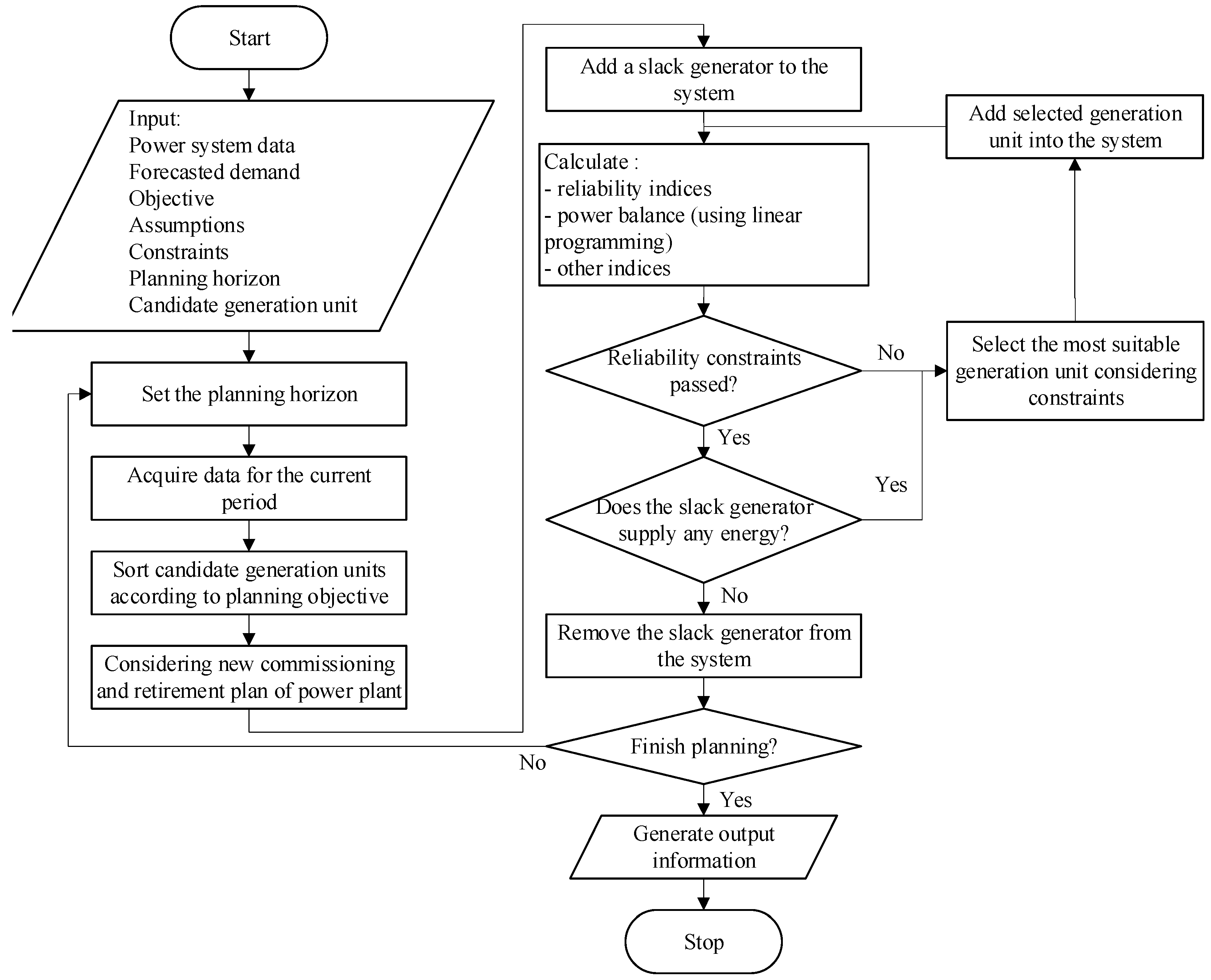
2.3. Simplification Process

In this section, a simplification process will be introduced to break the described multi-period MILP model down into a series of linear programming models. Firstly, the concept of simplification is discussed. Slack generation unit addition to the model is also introduced in order to guarantee that an optimal solution can be found for each iteration. The simplified model will be tested with the case study introduced in Section 3.

2.3.1. The Concept of Simplification

The object of this simplification is to reduce the number of variables and possible scenarios in the previously described multi-period MILP model. Three processes are applied to the described model:
  • Separate each month into multiple timeslots within the planning horizon to reduce the number of variables in a single calculation. By doing this, multiple MILP models will be used instead of a single multi-period MILP. Thus, multiple problems need to be iteratively solved and the optimal solution of the previous timeslot will be used as the initial condition of the next.
  • Separate generation expansion decisions from the MILP model. By doing this, the MILP model will be reduced to a linear programming model. Reliability constraints can also be removed from the linear programming model. However, a reliability index still needs to be calculated separately for generation expansion decisions. The remaining linear programming model in each specific month m of year y will be used for unit commitment problem and energy dispatch, which provides decision-making indices that will be subsequently used for generation expansion decisions.
  • Generation expansion decisions shall be made by comparing candidate generation units’ levelized average cost of electricity. With objective function shown in (1), adding generation units with the cheapest levelized average cost, considering the aforementioned constraints, still leads to near-optimal solutions for generation expansion planning, even if a full-scale optimization model is not used.
With these processes applied, a generation expansion plan can be created by iteratively solving a series of linear programming problems. Since the optimal solution for the previous timeslot needs to be used as the initial condition of the next, termination of iterative calculation needs to be prevented. However, a lack of available generation capacity or tight constraints could make optimal solutions impossible to find, leading to the termination of iterative calculations. To prevent this, the addition of slack generation units is presented, guaranteeing that optimal solutions can be found.

2.3.2. A Slack Generation Unit

Slack generation unit is unique generation unit added to the linear programming model to guarantee that there are optimal solutions that satisfy all hard constraints. However, since slack generation unit is not an actual generation unit available in the system, it must be dispatched to supply electricity only if all other existing generation units cannot satisfy all hard constraints. Dependence on slack generation units indicates that new generation capacity needs to be added to the system. The characteristics of slack generation unit, considering (1) to (19), must be as described below:
  • Availability: always available
  • Generating capacity: larger than peak demand of considered timeslot
  • Unit cost: much more than the most expensive unit
  • Fuel type and CO2 emissions: unspecified fuel type, no emission factor
The characteristics of slack generation unit can be changed in case the objective function is different or more constraints need to be considered.

2.3.3. Simplified Model

With the three processes in (Section 2.3.1) and addition of slack generation unit mentioned in (Section 2.3.2), a new flow chart of generation expansion planning can be generated, and is shown in Figure 2. The simplified linear programming model for the timeslot of month m of year y is shown in (20) to (31).
min   h = 1 H m f = 1 F j = 1 N f , y , m e f , j × P f , j , h
e f , j = F C f × H R f , j + V O M C f , j
subject to
h   :   f = 1 F j = 1 N f , y , m P f , j , h + s = 1 S j = 1 N s , y , m P d c h s , j , h · η d c h , s , j = L h + s = 1 S j = 1 N s , y , m P c h s , j , h η c h , s , j
f   :   h = 1 H m j = 1 N f , y , m P f , j , h     δ f , y , m × h = 1 H m f = 1 F j = 1 N f , y , m P f , j , h
f = 1 F j = 1 N f , y , m E F f × H R f , j × P f , j , h     ε y , m × f = 1 F j = 1 N f , y , m P f , j , h
h s j   :   E s , j , h = E s , j , h 1 + P c h s , j , h P d c h s , j , h
s j   :   E s , j , 1 = E s , j , m a x · S O C m i n , s , j
s j   :   E s , j , H m = E s , j , m a x · S O C m i n , s , j
h s j   :   P c h s , j , m i n     P c h s , j , h     P c h s , j , m a x
h s j   :   P d c h s , j , m i n     P d c h s , j , h     P d c h s , j , m a x
h f j   :   P f , j , m i n     P f , j , h     P f , j , m a x
h s j   :   E m a x , s , j · S O C m i n , s , j     E s , j , h     E m a x , s , j · S O C m a x , s , j
Unit commitment problems are considered monthly using the priority list method. It can be analyzed using (20)–(31). If any P f , j , h > 0 , these units are committed in hour h of the considering month. Equation (22) is used to guarantee that summation of output power from committed generation units and ESSs is equal to load at any hour. The remaining capacity, i.e., difference between installed capacity and output power of any unit that P f , j , h > 0 , can be considered as system’s spinning reserve. This level of simplification is acceptable for long-term planning problem with high uncertainty such as generation expansion planning since complicated unit commitment is not required in this stage of planning.
These energy dispatch problems are used to confirm whether hourly power balance constraints can be satisfied. They are also used to compare fuel mix index and also CO2 emission index with planning constraints.
The system reserve margin formula is shown in (32).
R M = f = 1 F j = 1 N m D F f , j × I C f , j P L P L
Due to the separation of generation expansion decisions, LOLE constraints can be separated from the optimization model shown in (20) to (31) and calculated directly. Therefore, LOLE, which is a better criterion representing system reliability, can also be used as a reliability criterion. The calculation method for system LOLE of the considered month and year starts from formulation of COPT as shown in Table 1, and load duration curve, as shown in Figure 3. With the formulated COPT and load duration curve, LOLE can be calculated using the following formula:
L O L E = i = 1 N p i · t L D C ( O i )
where N is number of states of COPT, pi is individual probability of outage capacity state i, and tLDC(Oi) is duration of the load loss due to the outage capacity Oi (hr).
This new method of LOLE calculation incorporating ESS is introduced in the next subsection.

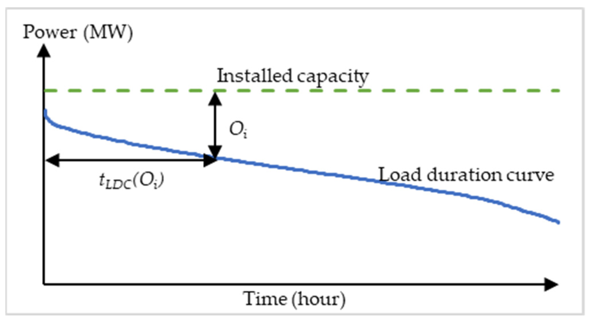
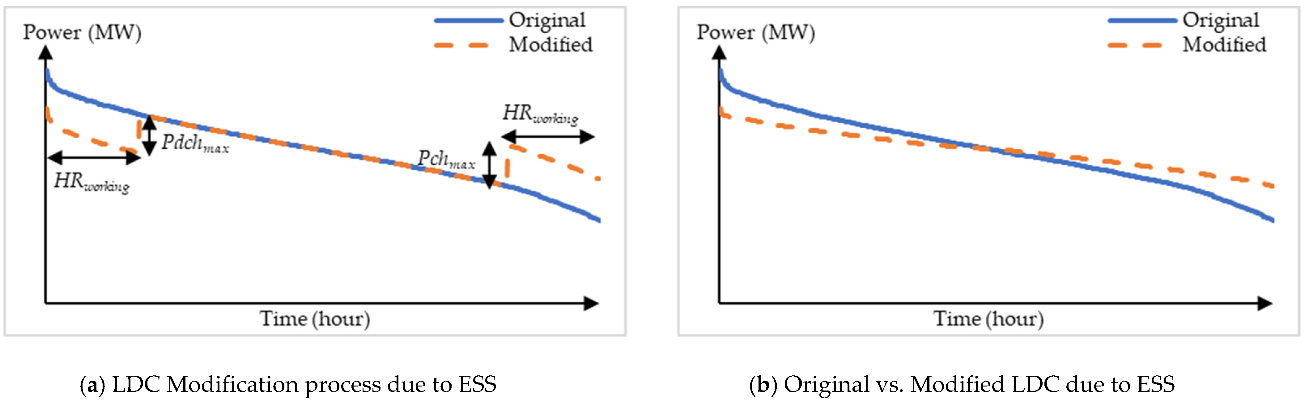
2.3.4. LOLE Calculation with ESS

To represent ESSs in LOLE calculations, the load duration curve is modified with the potential of each ESS by reduction of energy consumption during peak periods and increase of energy consumption during off-peak periods. Parameters of ESSs according to (34) to (38) need to be calculated and are used to modify the load duration curve as shown in Figure 4.
s   :   P S d c h s , j , m a x = P d c h s , j , m a x · η d c h , s , j
s   :   P S c h s , j , m a x       P c h s , j , m a x η c h , s , j  
s   :   H r w o r k i n g =   C y c l e s , j C r a t e s , j
where
C y c l e s , j =   m a x { 1 , h = 1 H m P c h s , j , h E m a x , s , j · D O D s , j }
D O D s , j =   S O C m a x , s , j S O C m i n , s , j
After the modification, the load duration curve may need to be rearranged and will be used to calculate LOLE using (33). Since profile of the LDC is modified, tLDC(Oi) will be changed to tLDC’(Oi). Thus, the obtained LOLE will represent the impact of ESS in the generation system. In case there are 2 or more ESS units, the method presented in Section 2.3.4 shall be done for every ESS unit before LOLE calculation.

2.3.5. Candidate Generation Capacity Selection

With the proposed simplification process and LOLE calculation, the GEP problem of a centralized power system is formulated. The decision-making process for generation expansion follows the flow chart in Figure 1. The linear programming problem involving cost minimization objective function (20) to (21) and constraints (22) to (31) are used to solve energy dispatch problems. Energy dispatch results, whether optimal solutions can be found or not, are considered in generation expansion decisions.
A reliability index, as either system reserve margin calculated from (32) or system LOLE calculated from (33), and energy dispatch results from linear programming are used as indicators for generation expansion decisions. More generation units need to be installed into the system when:
  • the system reserve margin is lower than the planning criteria, or
  • system LOLE is higher than the planning criteria, or
  • there is no optimal solution provided by linear programming, (in this case the slack generation units will be dispatched, instead).
If more generation units are needed, those with the lowest unit cost will be selected from the set of available generation types which pass all the defined constraints, such as fuel mix or maximum CO2 emissions. The selection process is shown in (39).
min   U n i t   c o s t = C f , k + e f , k , y
subject to
h = 1 H m j = 1 N f , y , m P f , j , h     δ f , y , m × h = 1 H m f = 1 F j = 1 N f , y , m P f , j , h

3. Case Study and Simulation Results

In this section, an overview of the case study will be provided. Firstly, planning constraints will be described, then the relevant models of generation unit will be provided. This information will be used with the proposed simplification process to create a generation expansion plan. This plan will be compared with Thailand’s actual generation expansion plan.
The proposed process is applied to a case study of Thailand’s generation expansion planning, which is called the “Power Development Plan” in Thailand. The selected case is Thailand’s power development plan 2010 revision 3 (PDP2010 Rev.3) [19], which was published in 2013 by the Ministry of Energy, Thailand. This version of the PDP was selected since it is the latest plan developed using a pure optimization process. Details of key assumptions, input data, and modeling of PDP2010 Rev.3 are described below.

3.1. Planning Constraints

The planning constraints and assumptions of PDP 2010 Rev.3 are as following:
  • Planning horizon: 2013–2030
  • Existing generation system as of December 2012 used as initial power generation system.
  • Consider reserve margin as reliability criteria. Reserve margin of the system shall not fall below 16%
  • Renewable energy source penetration in this plan is set in advance according to Thailand’s alternative energy development plan: AEDP 2012-2021 [34].
  • Average CO2 emission limited to 0.5 kgCO2/kWh within planning horizon.
  • Fuel used in electricity generation classified into ten types:
    • Bituminous
    • Diesel
    • Bunker oil
    • Import coal
    • Natural gas
    • Import hydro
    • Lignite
    • Import HVDE
    • Nuclear
    • Renewable
  • Maximum fuel mix ratio in 2030 of natural gas is 70% and bituminous is 13%

3.2. System Demand

Load modeling, a full-year hourly load curve, in PDP2010 Rev.3 is created from the actual hourly load curve of the selected base year, 2007, and load forecast data shown in Figure 5. The hourly load curve of the base year is scaled up based on the forecast peak load and energy of the considered year, assuming the constant minimum load to peak load ratio. Uncertainty of load forecast is also considered. Given that the probability of the forecasted value is 0.5 and the demand of the final year, 2030, can either increase or decrease by 3% with the probability of 0.25, uncertainty of load forecast of other years can be linearly modeled, accordingly.

3.3. Fuel Cost

Fuel price of every fuel is also forecasted and may vary throughout the planning horizon. In this paper, fuel price uncertainty is also considered. Given that the probability of the forecasted value is 0.5, the fuel price is allowed to either increase or decrease by 10% with the probability of 0.25.

3.4. Generation System

3.4.1. Generation Units in Generation Expansion Planning

The generation expansion plan according to PDP2010 Rev.3 runs from 2013 to 2030. Details of the plan will be provided in Appendix A. There are some generation units that have already been committed into the power system, since their providers already have contracts with Thailand’s generation system operator (prior to PDP2010 Rev.3 planning period). Also, some generation units, such as those using renewable energy sources, must be commissioned throughout the plan according to Thailand’s AEDP2012-2021 [34], and other related policies.
Although there are generation units committed throughout the planning horizon, there is still some excess demand that needs to be served. Therefore, a list of candidate generation units is also provided (Table 2).

3.4.2. Generation Unit Modeling

In PDP2010 Rev.3, generation units can be classified into three groups:
  • Renewable energy generation units with generation profiles:
Renewable energy generation units with specified generation profiles, such as solar power generation that can supply electricity depending on solar irradiance, will be modelled as generation units with hourly generation profiles to be used in hourly power balance Equation (22). The standard hourly generation profile of a 1-MW solar unit used in this paper can be found in [19]. It is created based on average hourly solar irradiance in a day for every month. Then this standard profile will be scaled to the capacity of each solar generation unit accordingly. Solar power generation uncertainty is also taken into consideration. The forecasted generation profile is given with the probability of 0.5 and it is allowed to fluctuate 10% around its forecasted profile with the probability of 0.25. With fuel price and renewable generation profile uncertainties, a joint probability density function can be created as shown in Table 3.
In this paper, wind and other RES power generation units are also modelled as generation units with constant generation profile as used in PDP2010rev3 [19]. However, in the latest version of Thailand’s PDP, PDP2018 revision 1 [35], all types of RES generation unit have their own generation profile.
2.
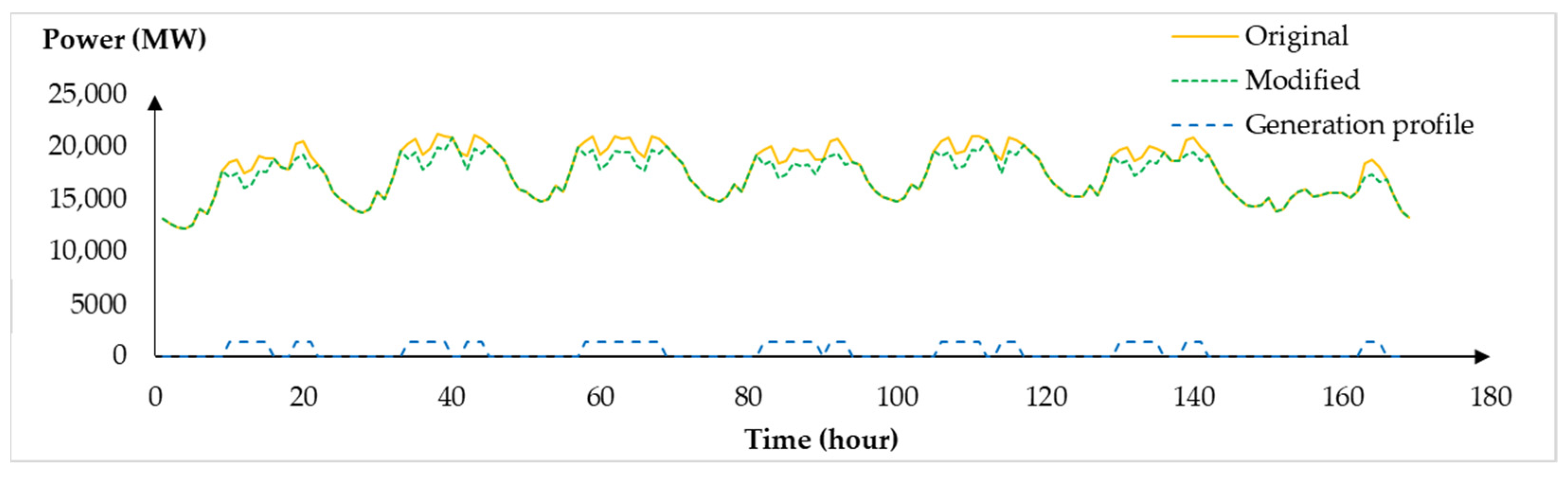
Peak cutting generation units:
Large hydropower generation units will be used as peak-cutting units since their power output is limited by the quantity of water in their reservoirs. This limitation is presented by each unit’s plant factor, which is varied throughout the year. Hydrogeneration units will supply power during peak load periods after the generation output of units in previous groups are considered. An example of the generation profile of hydropower generation is shown in Figure 6. In this study, both Thailand’s domestic and imported hydrogeneration units will be modelled as peak cutting generation units. The peak cutting method is done by the process of searching for peak hours in each day. Then each hydrogeneration unit will generate power to supply demand in those hours until reaching its daily energy limit.
3.
Dispatchable generation units:
Dispatchable generation units are large-scale generation units that consume commercial fuels. The generation output of these units can be dispatched by the system operator under constraints. The generation output of these units will be determined by linear programming Equations (19)–(30).
4.
Energy storage systems:
Hourly energy supplied and absorbed by ESSs in this case study also will be determined by linear programming Equations (19) to (30). There are two types of ESS in this case study: pumped hydro storage (PHS) and battery energy storage system (BESS). The parameters of these ESSs are shown in Table 4. Parameters of PHS unit is adopted from Lamtakong Jolabha Vadhana power plant in Thailand [36], which can be stored and supply power for eight hours in one cycle. Parameters of ESS unit is adopted from data sheet of BMZ energy storage systems model ESS 7.0/9.0 [37].

3.5. Result and Discussion

Using the data and assumptions of Thailand’s PDP2010 Rev.3, in Section 3.5.1 and Section 3.5.2, three generation expansion plans for Thailand’s electricity system have been developed, analyzed, and compared. Case 1 is the original PDP2010-Rev.3 in which all generation units, both committed and additional, have already been planned to be commissioned from 2013 to 2030. In Case 2, existing units and only generation units with power purchase agreements are considered as a base plan with the planning criteria described in [19]. Then, if necessary, additional units will be selected from the candidate list by the proposed method, to develop an alternative generation expansion plan from 2013 to 2030. Uncertainty of load, solar power generation, and fuel price are also incorporated in this case. In Section 3.5.1, Case 1 and Case 2 are compared to illustrate the consistency of results from the proposed method and the original plan. In Section 3.5.2, system indices of every scenario of Case 2 are discussed to illustrate the impact of uncertainty of demand, solar power generation, and fuel price on the generation expansion plan. In Section 3.5.3, Case 3 is used to illustrate the advantage of proposed method regarding the energy storage system (ESS). Several additional units from Case 2 will be replaced by BESS of the same size of installed capacity with one hour or higher storage capacity. The generation system indices including LOLE of Case 2 and Case 3 are calculated and compared to explore the impact of BESS.

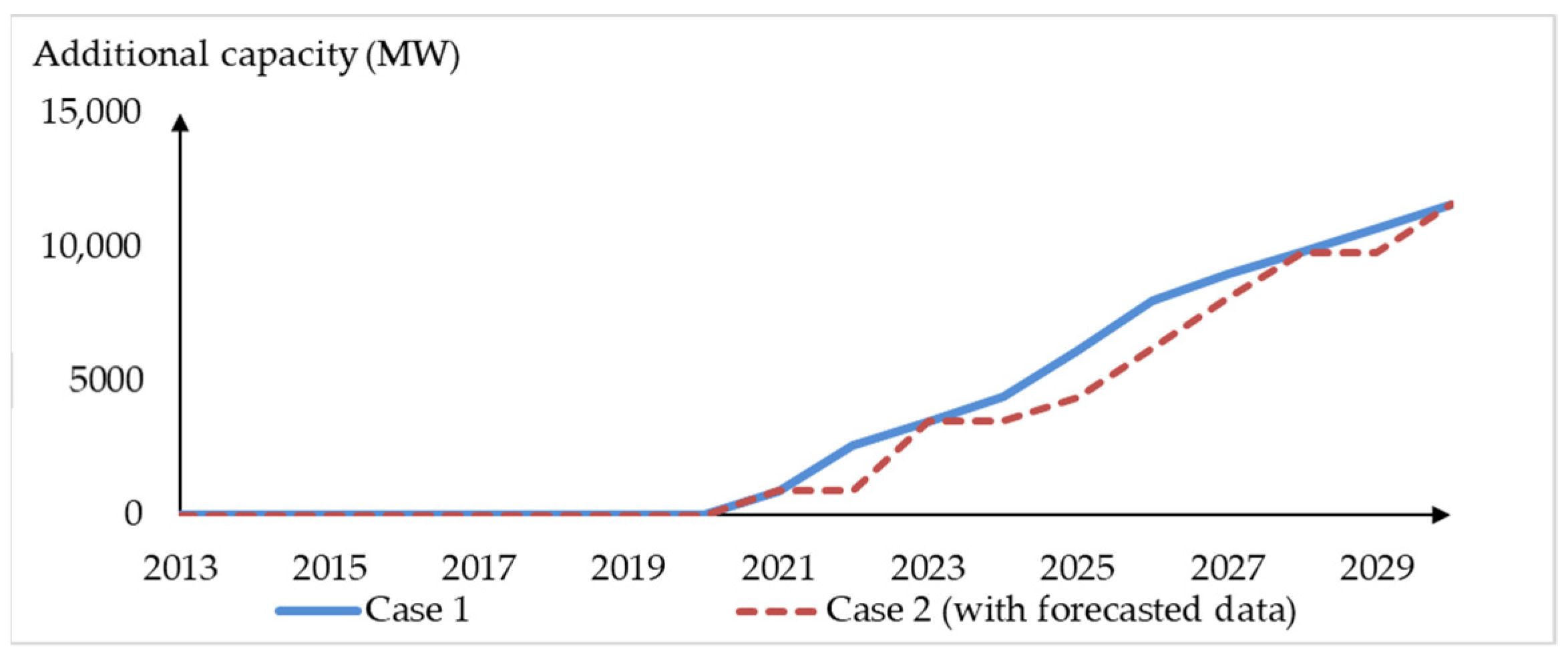
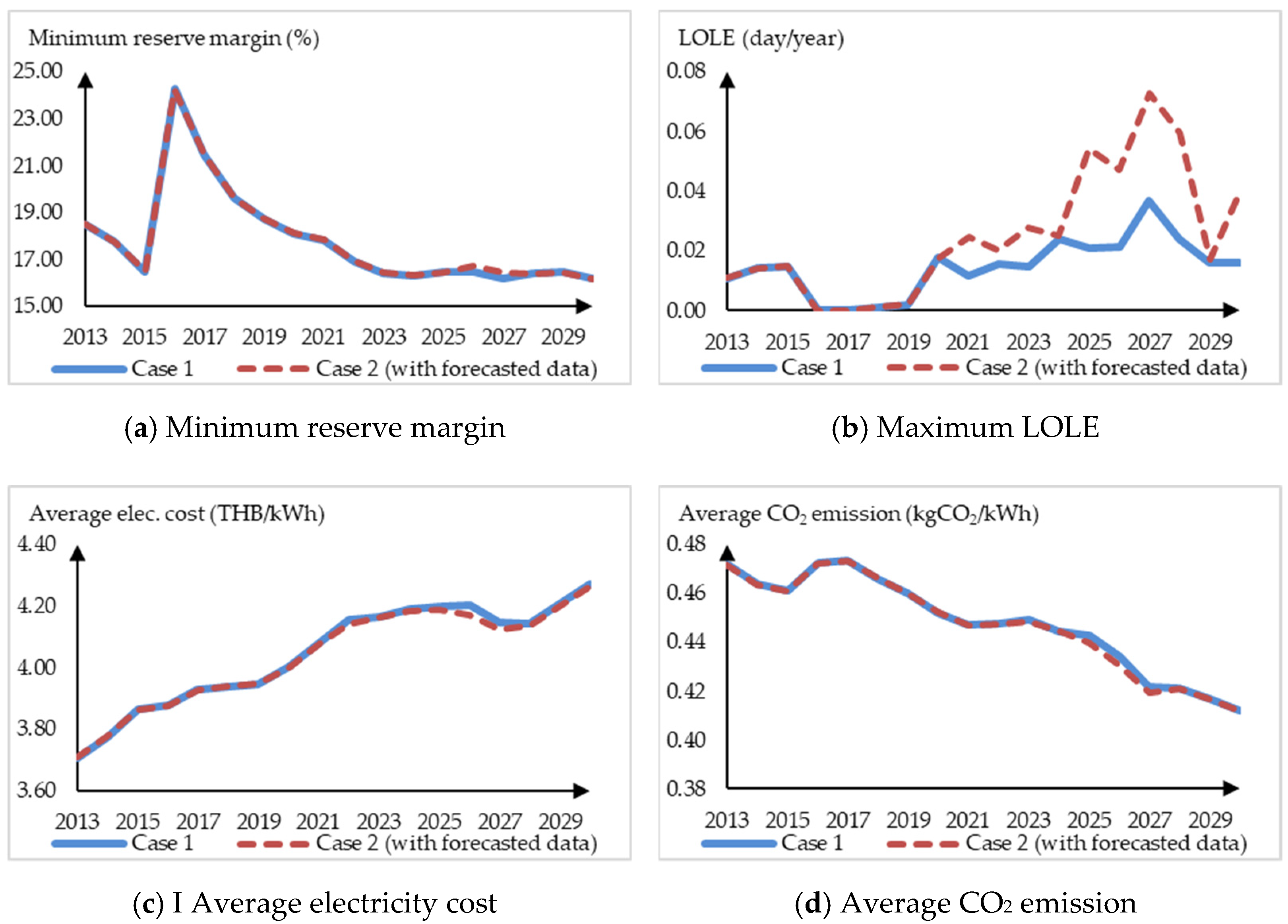
3.5.1. Verification of the Results from the Proposed Method

In this section, results obtained from Case 1 and from Case 2 using only forecasted data will be compared to show that the proposed method can provide almost the same results as those of the original plan. Considering forecasted demand and solar power generation, capacity of additional generation units for generation expansion plans at the end of each year of Case 1 and Case 2 are shown in Figure 7. Additionally, details of the planning results can be found in Table 5. In Table 5, only commission time of additional units is provided. The number shown in bracket is a commissioning month of additional units. With this result, system operator shall plan for the construction of generation units in advance to ensure that additional units can be commissioned as planned.
From Figure 7, although the additional capacity of Case 2 is not the same as Case 1 in every year, they are equal in 2023, 2028, and in the final year, 2030. Furthermore, from Table 5, both size and fuel type of additional power plants are quite similar. Thus, it indicates that the proposed method could provide nearly the same plan as Case 1. The difference between Case 1 and Case 2 in 2022 to 2029 might be caused by manual adjustments in the original plan by the policy maker. It is obviously seen that, in Case 1, there is a new unit added in every year unlike in Case 2, where a new unit is added only when needed. Also, new units in Case 1 are commissioned earlier.
Minimum reserve margins, LOLE, average electricity cost and average CO2 emission of Case 1 and Case 2 are shown in Figure 8. From Figure 8, reserve margin of Case 1 and Case 2 are mostly exactly the same, but slightly different in 2026 and 2027. Considering LOLE, since LOLE in this study is calculated monthly, annual LOLE can be obtained by accumulation of LOLE of 12 previous months. Case 1 has better reliability index since the new generation units in Case 1 are commissioned earlier compared to those of Case 2. However, both of them satisfy the requirement that LOLE must be less than one day per year. Thus, considering reserve margin and LOLE as the generation expansion decision-making indices, Case 1 and Case 2 provide almost the same result.
Due to early investment of new generation units in Case 1, the average electricity cost of Case 1 is slightly higher than that of Case 2 from 2021 to 2030. The average CO2 emission of Case 1 is also slightly higher than that of the Case 2 from 2025 to 2027. They are caused by the differences in commissioning sequence of additional generation unit as described earlier.
From Figure 8a, the reserve margin in 2015 to 2020 is quite high compared to the 16% target, since in the period there are several generation units that have already had the power purchase agreement with Thailand’s generation system operator as mentioned in Section 3.4.1.

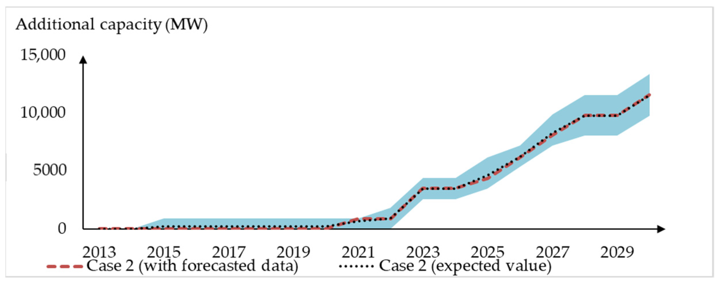
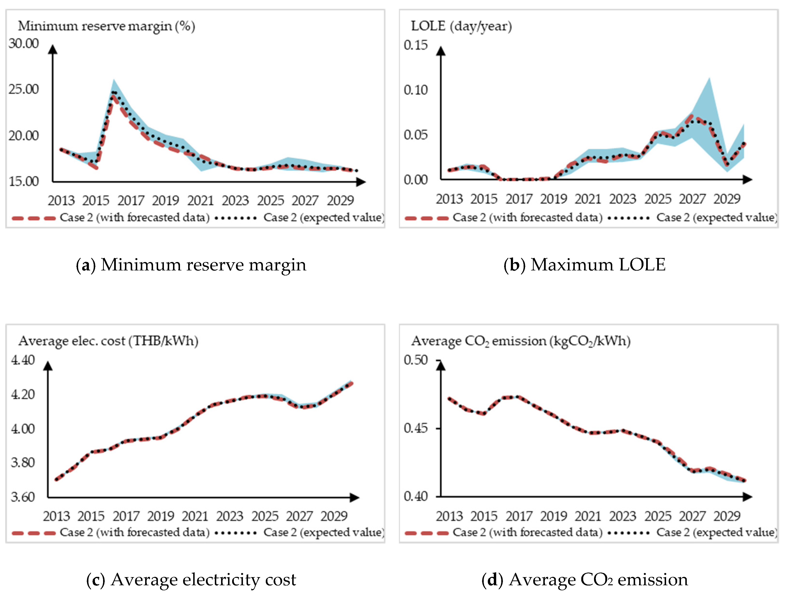
3.5.2. Generation Expansion Planning with Uncertainty

In this section, impact of uncertainties on generation expansion planning are investigated. All nine scenarios associated with load forecast error and solar power generation uncertainty stated in Table 3 are taken into consideration in Case 2. These uncertainties cause differences in generation expansion plan of each scenario. To illustrate the impact of uncertainties, in addition to the result obtained from using only forecasted data, minimum, maximum, as well as the expected values from all nine scenarios are also depicted in the generation expansion plan as a boundary shown with shaded area and a dotted line in Figure 9 and Figure 10. Additional generation capacity required to maintain the system reliability from 2013–2030 is shown in Figure 9 and also in Table 5. The minimum reserve margin, maximum LOLE, average electricity cost, and average CO2 emission are shown in Figure 10. respectively. It can be seen that the results obtained from using only forecasted data are a bit different from their corresponding expected values. They are just close to each other, but not exactly the same value, even though they are calculated from the symmetric joint probability distribution shown in Table 3.
Considering only fuel price uncertainty while other uncertainties are neglected, average cost of electricity and their corresponding boundary can be shown in Figure 11. In this case, average cost using only forecasted data is equal to its expected value.

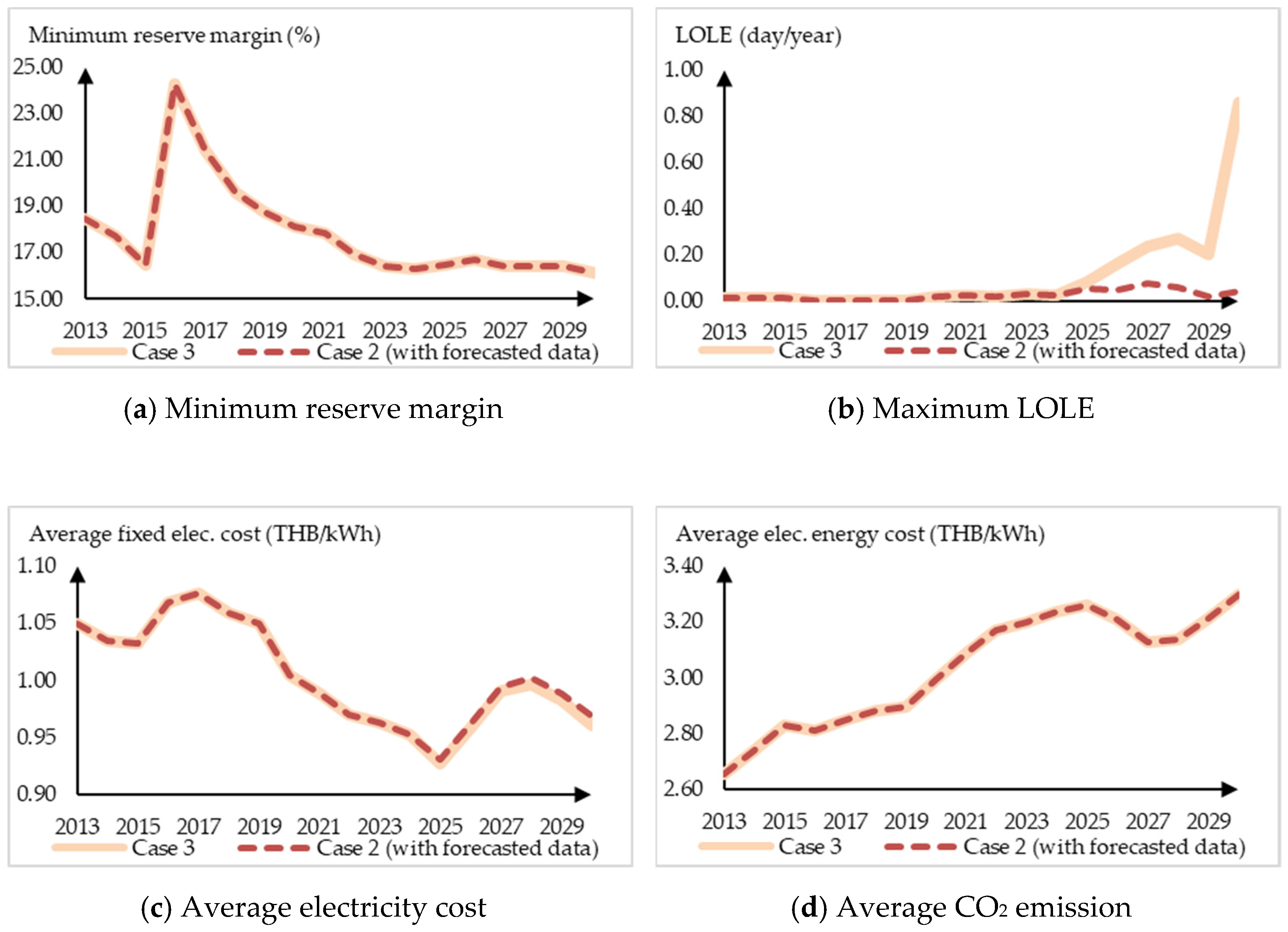
3.5.3. Generation Expansion Planning with ESS

In this section, ESS is incorporated into the test system to illustrate impact of ESS to generation expansion planning. System indices of Case 2 and Case 3, without uncertainty, are shown in Figure 12. Comparing Case 2 and Case 3, even though both cases have the same minimum reserve margin, the LOLE of Case 3 is higher (less reliable) since BESS and conventional generation units affect the LOLE index differently. The conventional generation unit in Case 2 affects the system’s generation model (COPT), but the BESS in Case 3 affects system’s load model as described in Section 2.3.4. Conventional generation unit can actually supply energy to the generation system if there is fuel. However, BESS does not provide any additional energy, and only performs load shifting. Additionally, charge and discharge process of BESS also creates energy loss. Thus, difference of their impact on system reliability reflects in the LOLE indices shown in Figure 12b.
As shown in Figure 12c, given that, from 2025 onward, the projection cost of investment of BESS is lower than that of the conventional power plant, average fixed generation cost of Case 3 is slightly lower than Case 2 since the total investment cost of the system is lower. Moreover, as shown in Figure 12d, the average CO2 emission of both cases are almost equal since energy supplied from BESS is generated from generation units in the system with the same average CO2 emission. However, due to loss in BESS, average CO2 emission of Case 3 is slightly higher than that of the Case 2.

3.5.4. Computational Cost

The generation expansion plans described herein were created using the MATLAB program. They are solved using a single 64-bit Windows 10 PC with i7-8750H CPU @2.20 GHz and 8.00 GB RAM. Linear programing was solved by IBM’s “cplexlp” function. Computational time for the 18-year planning horizon of a single problem was around four minutes. However, as Case 1 was developed by the Ministry of Energy of Thailand, the computation time was not disclosed in the plan. With the results outlined above, the proposed simplification process, with similar constraints, can provide nearly identical generation expansion plans to the PDP2010 rev.3 developed by the Ministry of Energy of Thailand with exceptional calculation speed (less than 5 min of computational time).

4. Conclusions

This paper proposes a method for generation expansion planning considering energy storage systems, renewable energy generation profiles, and full-year hourly power balance constraints. It is a simplification process to decompose a multi-period MILP generation expansion planning problem with realistic constraints and incorporate energy storage systems into multiple linear programming subproblems. With this process, individual unit characteristics with full-year hourly power balance constraints and renewable energy generation profiles can be considered in a multi-period linear programming model. This proposed method allows non-linear indices such as LOLE to be calculated during the decision-making process. The accuracy of the proposed method is clearly confirmed by the results shown in Section 3.5.1 with exceptional calculation speed. By their nature, generation expansion planning problem does not have a wide range of solutions due to several constraints that need to be considered. Therefore, with the same input, the simplified process described in Section 2.3 provides almost identical solution compared to the multi-period MILP described in Section 2.2. With less complexity and computational time, many complicated constraints can be taken into consideration. For instance, full-year hourly power balance constraints with renewable energy generation profiles, fuel mixes and CO2 emissions. These constraints can vary each season or each year, allowing more flexibility in long term generation expansion planning. Furthermore, with less computation time, it allows uncertainties to be taken into consideration. Multiple GEP using different assumptions with corresponding probabilities can be solved. The impact of installation of ESSs on system reliability can also be obviously seen in the LOLE.
The proposed method still has some limitations. As shown in Figure 1, only generation system is considered. Transmission network is neglected. However, actual generation system is typically divided into several regions connected with major tie-lines. Each region may also have its own constraints, e.g., available fuel options, difference renewable energy profiles, regional load profile, etc. In future work, we will include more realistic constraints to represent issues that need to be considered in modern generation expansion planning, e.g., different reliability criteria, regional constraints, major transmission network constraints, response of each power plant types, etc.

Author Contributions

Conceptualization, R.D. and K.A.; Methodology, R.D. and K.A.; Software, R.D.; Validation, K.A.; Formal analysis, R.D.; Investigation, K.A.; Resources, R.D. and K.A.; Data curation, R.D.; Writing—original draft preparation, R.D.; Writing—review and editing, K.A.; Visualization, R.D.; Supervision, K.A. All authors have read and agreed to the published version of the manuscript.

Funding

This research received no external funding. The APC will be partially funded by Energy Research Institute, Chulalongkorn University.

Conflicts of Interest

The authors declare no conflict of interest.

Nomenclature

Indices
ffuel type
hhour in considering month
iState of capacity outage Oi
jexisting generation unit and ESS in current planning horizon
knew generation unit added into current planning horizon
mmonth in planning horizon
sESS type
yyear in planning horizon
Parameters
Cinvj,kinvestment capital cost of generation unit k which use fuel type f (THB/MW)
Cf,kfixed cost per MW of candidate generation unit k which use fuel type f (THB/MW)
Crates,jc-rate of ESS type s unit j (MW/MWh)
DFf,jdependable factor of generation unit j of fuel type f (%)
ef,j,yvariable cost of electricity generated from generation unit j of fuel type f in year y (THB/MWh)
EFfemission factor of fuel type f (kgCO2/Btu)
Es,j,y,m,hstored energy in ESS type s unit j at hour h month m year y (MWh)
FCf,yfuel cost of fuel type f in year y (THB/Btu)
FOMCf,kFixed operation and maintenance cost of generation unit k which use fuel type f (THB/MW/year)
FORf,j,y,mforced outage rate of generation unit j which use fuel type f of month m of year y (%)
Hmnumber of hours in month m, i.e., 744 h in January, 720 h in April
HRf,jheat rate of generation unit j that use fuel type f (Btu/MWh)
LDCy,mLoad duration of month m of year y
LOLEloss of load expectation (day/year)
LTf,klifetime of new generation unit k which use fuel type f (year)
Ly,m,hload of hour h in month m of year y (MW)
Nf,y,mnumber of existing generation unit of fuel type f in month m of year y
Ns,y,mnumber of existing ESS unit of type s in month m of year y
Nf,y,mnumber of new generation unit of fuel type f added in the system in month m of year y
OiOutage capacity i (MW)
Pchs,j,maxmaximum internal power input (charge state) of ESS of type s unit j (MW)
Pchs,j,minminimum internal power input (charge state) of ESS of type s unit j (MW)
Pdchs,j,maxmaximum internal power output (discharge state) of ESS of type s unit j (MW)
Pdchs,j,minminimum internal power output (discharge state) of ESS of type s unit j (MW)
Pf,j,maxmaximum power output of generation unit j that use fuel type f (MW)
Pf,j,minminimum power output of generation unit j that use fuel type f (MW)
piindividual probability of outage capacity state i
PLy,mpeak load of month m of year y (MW)
PSchs,j,maxmaximum system power input (charge state) of ESS unit j (MW)
PSdchs,j,maxmaximum system power output (discharge state) of ESS unit j (MW)
rdiscount rate (%)
RMreserve margin (%)
SOCmax,s,jmaximum state of charge of ESS type s unit j (%)
SOCmin,s,jminimum state of charge of ESS type s unit j (%)
tLDC(Oi)duration of the load loss due to the outage capacity Oi (hr) in load duration curve (LDC)
tLDC’(Oi)duration of the load loss due to the outage capacity Oi (hr) in modified load duration curve (LDC’)
VOMCf,jvariable operation and maintenance cost of generation unit j of fuel type f (THB/MWh)
δf,y,mfuel ratio of fuel type f in year y (%)
εy,mmaximum average CO2 emission of year y (kgCO2/MWh)
ηch,s,jcharging efficiency of ESS type s unit j (%)
ηdch,s,jdischarging efficiency of ESS type s unit j (%)
Variable
ICf,k,y,mInstalled capacity of candidate generation unit k which use fuel type f commissioned in month m of year y (MW)
Pchs,j,y,m,hSelf-power absorbed by ESS type s unit j in hour h of month m of year y (MW)
Pdchs,j,y,m,hSelf-power supplied by ESS type s unit j in hour h of month m of year y (MW)
Pf,j,y,m,hPower generated by generation unit j which use fuel type f in hour h of month m of year y (MW)

Appendix A

Table A1. Thailand’s power generation system as of December 2012.
Fuel TypeNumber (Unit)Total Capacity (MW)Lifetime (Years)Heat Rate (Btu/kWh)
bituminous82376.0025–308300–9100
diesel14.402510,400
oil2320.0021–308300–10,400
import coal----
import HVDC1300.0025-
import hydro52104.6025–50-
Lignite102180.0030–3910,600–11,500
natural gas6521,796.3020–316800–10,300
nuclear----
renewableN/A4684.1021–50-
PHS1500.0050-
Table A2. Renewable energy generation unit as of December 2012.
Fuel TypeTotal Cap. (MW)Lifetime (Years)
hydro2967.9825–50
solar303.0325
wind249.9025
biomass1028.6021–25
biogas110.2025
waste22.4025
geothermal2.0025
Table A3. Net committed generation capacity (commission and retire) of PDP2010Rev3 (MW).
YearBituminousDieselOilImport CoalImport HydroLigniteNatural GasPHS
2013 1186.00
2014 3436.90
−1052.00
2015 982.00 3056.90
−1175.10
2016270.00 491.00 1370.80
−478.20
2017270.00 900.00
−494.00
500.00
2018 659.00 720.90
−680.50
2019800.00
−5.00
1220.00 724.80
−180.00
2020 90.00
−1521.00
2021 300.00 1080.90
−200.00
2022 300.00 1084.80
−150.00
2023 300.00 1980.00
−2863.00
2024
−270.00
300.00 1980.90
−360.00
2025
−90.00
300.00 1084.8
−2330.00
2026 300.00 1080.00
2027 300.00 1980.90
−2617.00
2028 250.00 300.00 1804.80
−1289.00
2029 250.00 300.00
−270.00
900.00
2030 250.00 300.00
−126.00

−270.00
0.90
Table A4. Net committed generating capacity of RES of PDP2010Rev3 (MW).
YearSmall HydroSolarWindBiomassBiogasWaste
201319.20375.8014.00574.50-56.00
20140.50181.10263.60206.801.2012.80
201551.80191.10302.90180.502.3022.80
20165.20130.10163.10175.302.3032.80
201722.00130.10163.10175.302.3041.80
201823.60130.007.40184.502.4041.80
20193.50151.00117.80179.802.4041.80
20204.70151.008.20234.00
−8.00
2.5041.90
20211.50201.008.60186.002.5041.90
20221.30220.109.0053.702.501.90
20233.50220.1019.5032.802.601.90
20242.20220.109.9038.60
−49.80
2.601.90
20253.30220.0010.4021.20
−56.00
2.602.00
20261.00221.0011.0016.80
−5.00
2.702.00
202712.00220.1061.5016.90
−7.00
2.702.00
202817.30221.0012.1014.40
−103.00
2.802.00
20291.00223.0022.7014.502.802.00
20301.00230.0043.3014.70
−20.00
2.802.10

References

  1. Nie, S.; Huang, Z.C.; Huang, G.H.; Yu, L.; Liu, J. Optimization of electric power systems with cost minimization and environmental-impact mitigation under multiple uncertainties. Appl. Energy 2018, 221, 249–267. [Google Scholar] [CrossRef]
  2. Koltsaklis, N.E.; Dagoumas, A.S. State-of-the-art generation expansion planning: A review. Appl. Energy 2018, 230, 563–589. [Google Scholar] [CrossRef]
  3. Oree, V.; Sayed Hassen, S.Z.; Fleming, P.J. Generation expansion planning optimisation with renewable energy integration: A review. Renew. Sustain. Energy Rev. 2017, 69, 790–803. [Google Scholar] [CrossRef]
  4. Saber, H.; Moeini-Aghtaie, M.; Ehsan, M. Developing a multi-objective framework for expansion planning studies of distributed energy storage systems (DESSs). Energy 2018, 157, 1079–1089. [Google Scholar] [CrossRef]
  5. Massé, P.; Gibrat, R. Application of linear programming to investments in the electric power industry. Manag. Sci. 1957, 3, 149–166. [Google Scholar] [CrossRef]
  6. Heuberger, C.F.; Rubin, E.S.; Staffell, I.; Shah, N.; Mac Dowell, N. Power capacity expansion planning considering endogenous technology cost learning. Appl. Energy 2017, 204, 831–845. [Google Scholar] [CrossRef]
  7. Koltsaklis, N.E.; Dagoumas, A.S.; Kopanos, G.M.; Pistikopoulos, E.N.; Georgiadis, M.C. A spatial multi-period long-term energy planning model: A case study of the Greek power system. Appl. Energy 2014, 115, 456–482. [Google Scholar] [CrossRef]
  8. Quiroga, D.; Sauma, E.; Pozo, D. Power system expansion planning under global and local emission mitigation policies. Appl. Energy 2019, 239, 1250–1264. [Google Scholar] [CrossRef]
  9. Zhang, N.; Hu, Z.; Shen, B.; He, G.; Zheng, Y. An integrated source-grid-load planning model at the macro level: Case study for China’s power sector. Energy 2017, 126, 231–246. [Google Scholar] [CrossRef]
  10. Hemmati, R.; Saboori, H.; Jirdehi, M.A. Multistage generation expansion planning incorporating large scale energy storage systems and environmental pollution. Renew. Energy 2016, 97, 636–645. [Google Scholar] [CrossRef]
  11. Alizadeh, B.; Jadid, S. A dynamic model for coordination of generation and transmission expansion planning in power systems. Int. J. Electr. Power Energy Syst. 2015, 65, 408–418. [Google Scholar] [CrossRef]
  12. Booth, R.R. Optimal generation planning considering uncertainty. IEEE Trans. Power Appar. Syst. 1972, PAS-91, 70–77. [Google Scholar] [CrossRef]
  13. Su, C.T.; Lii, G.R.; Chen, J.J. Long-term generation expansion planning employing dynamic programming and fuzzy techniques. In Proceedings of the IEEE International Conference on Industrial Technology, Goa, India, 19–22 January 2000; pp. 644–649. [Google Scholar] [CrossRef]
  14. Neshat, N.; Amin-Naseri, M.R. Cleaner power generation through market-driven generation expansion planning: An agent-based hybrid framework of game theory and Particle Swarm Optimization. J. Clean. Prod. 2015, 105, 206–217. [Google Scholar] [CrossRef]
  15. Gupta, N.; Khosravy, M.; Patel, N.; Senjyu, T. A Bi-Level Evolutionary Optimization for Coordinated Transmission Expansion Planning. IEEE Access 2018, 6, 48455–48477. [Google Scholar] [CrossRef]
  16. Gupta, N.; Shekhar, R.; Kalra, P.K. Computationally efficient composite transmission expansion planning: A Pareto optimal approach for techno-economic solution. Int. J. Electr. Power Energy Syst. 2014, 63, 917–926. [Google Scholar] [CrossRef]
  17. Gacitua, L.; Gallegos, P.; Henriquez-Auba, R.; Lorca; Negrete-Pincetic, M.; Olivares, D.; Valenzuela, A.; Wenzel, G. A comprehensive review on expansion planning: Models and tools for energy policy analysis. Renew. Sustain. Energy Rev. 2018, 98, 346–360. [Google Scholar] [CrossRef]
  18. Korea Power Exchange. The 7th Basic Plan for Long-term Electricity Supply and Demand (2015–2019). Available online: https://www.kpx.or.kr/eng/selectBbsNttView.do?key=328&bbsNo=199&nttNo=14547 (accessed on 31 August 2021).
  19. Energy Policy and Planning Office. Summary of Thailand Power Development plan (PDP2010: Revision 3). Available online: https://www.erc.or.th/ERCWeb2/Upload/Document/PDP2010-Rev3-Cab19Jun2012-E.pdf (accessed on 31 August 2021).
  20. Park, H.; Baldick, R. Multi-year stochastic generation capacity expansion planning under environmental energy policy. Appl. Energy 2016, 183, 737–745. [Google Scholar] [CrossRef]
  21. Afful-Dadzie, A.; Afful-Dadzie, E.; Awudu, I.; Banuro, J.K. Power generation capacity planning under budget constraint in developing countries. Appl. Energy 2017, 188, 71–82. [Google Scholar] [CrossRef]
  22. Guerra, O.J.; Tejada, D.A.; Reklaitis, G.V. An optimization framework for the integrated planning of generation and transmission expansion in interconnected power systems. Appl. Energy 2016, 170, 1–21. [Google Scholar] [CrossRef]
  23. Koltsaklis, N.E.; Georgiadis, M.C. A multi-period, multi-regional generation expansion planning model incorporating unit commitment constraints. Appl. Energy 2015, 158, 310–331. [Google Scholar] [CrossRef]
  24. Wierzbowski, M.; Lyzwa, W.; Musial, I. MILP model for long-term energy mix planning with consideration of power system reserves. Appl. Energy 2016, 169, 93–111. [Google Scholar] [CrossRef] [Green Version]
  25. Belderbos, A.; Delarue, E. Accounting for flexibility in power system planning with renewables. Int. J. Electr. Power Energy Syst. 2015, 71, 33–41. [Google Scholar] [CrossRef] [Green Version]
  26. Chen, X.; Lv, J.; McElroy, M.B.; Han, X.; Nielsen, C.P.; Wen, J. Power system capacity expansion under higher penetration of renewables considering flexibility constraints and low carbon policies. IEEE Trans. Power Syst. 2018, 33, 6240–6253. [Google Scholar] [CrossRef]
  27. Opathella, C.; Elkasrawy, A.; Adel Mohamed, A.; Venkatesh, B. MILP formulation for generation and storage asset sizing and sitting for reliability constrained system planning. Int. J. Electr. Power Energy Syst. 2020, 116, 105529. [Google Scholar] [CrossRef]
  28. Billinton, R.; Allan, R. Reliability Evaluation of Power Systems; Pitman Advanced Publishing Program: London, UK, 1984; ISBN 0273084852. [Google Scholar]
  29. Aghaei, J.; Akbari, M.A.; Roosta, A.; Baharvandi, A. Multiobjective generation expansion planning considering power system adequacy. Electr. Power Syst. Res. 2013, 102, 8–19. [Google Scholar] [CrossRef]
  30. Pudjianto, D.; Aunedi, M.; Djapic, P.; Strbac, G. Whole-Systems assessment of the value of energy storage in low-carbon electricity systems. IEEE Trans. Smart Grid 2014, 5, 1098–1109. [Google Scholar] [CrossRef]
  31. Hemmati, R.; Saboori, H.; Siano, P. Coordinated short-term scheduling and long-term expansion planning in microgrids incorporating renewable energy resources and energy storage systems. Energy 2017, 134, 699–708. [Google Scholar] [CrossRef]
  32. Choi, J.; Park, W.K.; Lee, I.W. Economic dispatch of multiple energy storage systems under different characteristics. Energy Procedia 2017, 141, 216–221. [Google Scholar] [CrossRef]
  33. Xiong, P.; Singh, C. Optimal planning of storage in power systems integrated with wind power generation. IEEE Trans. Sustain. Energy 2016, 7, 232–240. [Google Scholar] [CrossRef]
  34. Sutabutr, T. Alternative Energy Development Plan (2012–2021). Available online: http://www.sert.nu.ac.th/IIRE/FP_V7N1(1).pdf (accessed on 28 August 2021).
  35. Ministry of Energy Thailand: Thailand’s Power Development Plan (PDP) 2018 Rev. 1. Available online: https://policy.asiapacificenergy.org/node/4347/portal (accessed on 31 August 2021).
  36. Electricity Generating Authority of Thailand Lamtakong Jolabha Vadhana Power Plant. Available online: https://www.egat.co.th/en/information/power-plants-and-dams?view=article&id=46 (accessed on 28 August 2021).
  37. BMZ Energy Storage System Data Sheet—ESS 7.0/9.0. Available online: https://d3g1qce46u5dao.cloudfront.net/data_sheet/170622_bmz_ess_70_datasheet_en_v032017.pdf (accessed on 28 August 2021).
Figure 1. Conventional system model.
Energies 14 05733 g001
Figure 2. Flow chart of generation expansion planning with simplified process.
Energies 14 05733 g002
Figure 3. Load duration curve with tLDC(Oi) calculation.
Energies 14 05733 g003
Figure 4. Load duration curve modification by potential of ESSs.
Energies 14 05733 g004
Figure 5. Forecasted peak load and energy demand of PDP2010 Rev.3.
Energies 14 05733 g005
Figure 6. Example of hydrogeneration profile in one week.
Energies 14 05733 g006
Figure 7. Additional capacity for generation expansion plans.
Energies 14 05733 g007
Figure 8. Comparison of generation system indices of Case 1 and Case 2.
Energies 14 05733 g008
Figure 9. Additional capacity for generation expansion plans with load and solar uncertainty.
Energies 14 05733 g009
Figure 10. Generation system indices of Case 2 with uncertainty.
Energies 14 05733 g010
Figure 11. Average cost with fuel price uncertainty.
Energies 14 05733 g011
Figure 12. Comparison of generation system indices of Case 2 and Case 3.
Energies 14 05733 g012
Table 1. Example of Capacity Outage Probability Table.
Capacity Outage (MW)Capacity Available (MW)State Probability
O1Installed capacity—O1p1
O2Installed capacity—O2p2
OiInstalled capacity—Oipi
ONInstalled capacity—ONpN
Table 2. Candidate units for PDP2010 Rev.3.
Generation UnitFuel TypeCapacity
(MW)
Lifetime
(years)
Heat Rate
(Btu/kWh)
Remark
Coal fired thermalBituminous800308650Unlimited
Combined cycleNatural gas900256800Unlimited
NuclearNuclear10006010,950Unlimited
Table 3. Joint probability density function for load and solar power generation uncertainties.
Parameters% of Forecasted Load (Associated Probability)
97% (0.25)100% (0.5)103% (0.25)
% of solar power generation
(associated probability)
90% (0.25)0.06250.1250.0625
100% (0.5)0.1250.250.125
110% (0.25)0.06250.1250.0625
Table 4. Parameters of ESSs in this case study.
TypeC-Rate
(MW/MWh)
Charging
Efficiency (%)
Discharging Efficiency (%)Minimum
State of Charge (%)
Maximum
State of Charge (%)
PHS0.12586.6%86.6%0.0%100.0%
BESS197.5%97.5%10.0%90.0%
Table 5. List of additional units.
YearResults for Section 3.5.1Results for Section 3.5.2
Case 1Case 2 (w/Forecasted)Case 2 MinCase 2 Max
2015 (4) NG 900 MW
2021(1) NG 900 MW(4) NG 900 MW
2022(6) Coal 800 MW
(6) NG 900 MW
(4) NG 900 MW
2023(1) NG 900 MW(3) Coal 800 MW
(3) NG 900 MW
(4) NG 900 MW
(3) Coal 800 MW
(3) NG 900 MW
(4) NG 900 MW
(3) Coal 800 MW
(3) NG 900 MW
(4) NG 900 MW
2024(6) NG 900 MW
2025(6) Coal 800 MW
(6) NG 900 MW
(4) NG 900 MW(4) NG 900 MW(4) NG 900 MW
(4) NG 900 MW
2026(6) Nuclear 1000 MW
(6) NG 900 MW
(3) Nuclear 1000 MW
(4) Coal 800 MW
(3) Nuclear 1000 MW
(4) NG 900 MW
(4) Nuclear 1000 MW
 
2027(6) Nuclear 1000 MW(3) Nuclear 1000 MW
(4) NG 900 MW
(3) Nuclear 1000 MW
(4) Coal 800 MW
(3) Nuclear 1000 MW
(4) Coal 800 MW
(4) NG 900 MW
2028(1) Coal 800 MW(3) Coal 800 MW
(4) NG 900 MW
(4) NG 900 MW
 
(3) Coal 800 MW
(4) NG 900 MW
2029(6) NG 900 MW
2030(1) NG 900 MW(3) NG 900 MW
(4) NG 900 MW
(3) Coal 800 MW
(4) NG 900 MW
(3) NG 900 MW
(4) NG 900 MW
Total11,600 MW11,600 MW9800 MW13,400 MW
Publisher’s Note: MDPI stays neutral with regard to jurisdictional claims in published maps and institutional affiliations.

