Abstract
A comparative analysis of energy poverty transitions and persistence can provide valuable suggestions for long-term policy actions. This study examines the dynamics of energy poverty in 17 European countries based on the longitudinal household data from the EU Survey on Income and Living Conditions, waves 2015–2018. The study pursues two goals. First, we explore households’ chances of transitioning in and out of energy poverty in each country following the discrete-time Markov process. On average, the probability to stay in energy poverty is 51.5%, and there is a lot of heterogeneity across countries. Households in Bulgaria, Greece, Romania, and Lithuania are quite close to the energy poverty trap. Second, we identify factors that help energy-poor households leave energy poverty. Demographic, technical, and socio-economic factors are the drivers in escaping energy poverty, which suggests common EU policy.
1. Introduction
Facing the transition to a carbon-neutral economy, in 2019 the EU adopted a set of legislative acts entitled the Clean Energy for all Europeans Package. Recognizing the importance of clean energy for economic growth and job creation (COM/2016/0860), EU countries joined their efforts to boost the creation of the Energy Union. A series of policy actions on counteracting energy poverty were adopted in EU countries [1] following the Clean Energy for all Europeans Package. With the interest of consumers being placed at the center of the redesigned energy market, the EU committed to energy poverty alleviation and the protection of vulnerable consumers (Energy Poverty 2020). In general terms, energy poverty is defined as a lack of access to modern energy services, however, the precise definition of energy poverty depends on the measurement technique. In our study energy poverty denotes the inability to keep home warm. The Governance Regulation (Regulation (EU) 2018/1999) and the Electricity Directive (Directive (EU) 2019/944) oblige member states to measure, monitor, and report on the assistance to energy-poor households, and to outline policy actions supporting the energy poor in the national energy and climate plans, especially in countries with a significant number of the energy poor. As reported by the EU Energy Poverty Observatory (2020), about 50 million households are at present facing challenges of energy poverty. The recent analysis of the structural energy poverty vulnerability [2] identifies those regions and countries on the EU map in which the problem is particularly acute.
The initiatives aimed at energy poverty reduction at the EU level necessitate a thorough understanding of the nature of energy poverty in all member states. While there are plenty of studies on energy poverty prevalence, both single-country [3,4,5] and comparative studies [6,7,8], the cross-country assessment of energy poverty persistence in Europe has not been done yet. In particular, it is not known whether the persistence of energy poverty is the same or different in all European countries. Detecting potential differences in the persistence of EP enables a better understanding of the phenomenon, identifies factors that facilitate the escape from EP, and identifies effective social policy tools used by different EU countries. We intend to cover this gap. We examine the persistence of energy poverty in 17 European countries, giving European politicians new insights into how energy poverty is developing in the perspective of four years. The following countries are considered: Belgium (BE), Bulgaria (BG), Croatia (HR), Cyprus (CY), Czechia (CZ), France (FR), Germany (DE), Greece (EL), Hungary (HU), Italy (IT), Latvia (LV), Lithuania (LT), Malta (MT), Poland (PL), Romania (RO), Slovenia (SI), and Spain (ES). The study answers two research questions:
- (1)
- How difficult is it for households in 17 European countries to escape energy poverty?
- (2)
- What factors determine success in escaping energy poverty?
There are two reasons behind the study. First, by providing evidence on energy poverty persistence in Europe, the analysis can be beneficial in formulating high-level policy and long-term strategies within the EU. Energy poverty, as well as poverty, is a stochastic phenomenon [9]. The level of energy poverty measured at a point of time provides no information on how easily the problem can be overcome and how European countries differ in terms of energy poverty persistence. Second, by identifying universal factors triggering escape from energy poverty, the study helps to find common points in national energy poverty policies. Focusing on the energy poor households from all countries, we could detect what helps them to get out of the predicament and, at the same time, capture the variation attributed to the among-country random effect.
Although member states define and measure energy poverty at their discretion, several suggested indicators and definitions are published [10,11] and recommended by the European Commission (2020/1563). The best known measures of energy poverty include expenditure-based and subjective indicators [12]. In this study, we rely on a subjective energy poverty indicator, i.e., the inability to keep homes warm, following the approach indicated by, among others, the European Commission (2020) and the Council of Europe Development Bank (2019). The ability-to-keep-home-warm indicator belongs to subjective metrics and is available in the EU-SILC database, i.e., the major source of the primary consensual energy poverty indicators in the EU. This indicator is frequently used in the comparative analysis of energy poverty in Europe [8,13]. Being aware of the drawbacks of subjective indicators, such as biasness [14] or inconsistency, we believe the inability-to-keep-home-warm indicator reveals people’s perceptions and is useful in studying complex issues [15] in multiple locations. This indicator does not require additional assumptions or expert-based assessment [16], which might be different for different countries and provides the best fit for the data and the purpose of our analysis.
The analysis is carried out in two steps following the research questions of the study. We use panel data from the EU-SILC questionnaire collected by Eurostat on an annual basis. Our choice of countries is determined by the availability of variables and the size of the energy-poor households sample in a base year. Only countries with more than 100 energy-poor households in 2015 are considered.
In the first step, we focus on all households from each country separately and analyze two states in which households can stay: energy poverty and non-energy poverty, and then examine the chances of moving between them. The transition probability in each country is estimated using the discrete-time Markov process. We assess the persistence of energy poverty as the probability to remain in the same condition in 4 years. The first-step transition probability matrices obtained are next used in the clustering procedure. To identify groups with similar transition paths we apply hierarchical and k-means clustering.
In the second step, we look at energy-poverty households from all countries and identify the factors that help these households move from energy poverty in four years. In identifying the determinants of escaping energy poverty, the study relies on the binomial mixed-effect regression. To account for the differences between countries, we include a varying among-countries intercept as a random effect of the model. We control for poverty, building characteristics, age, education, employment status, size of the family, and tenure status.
Our main findings confirm regional differences within Europe in terms of energy poverty persistence. Three groups of countries with similar transition probability paths are discovered, of which Bulgaria, Greece, Lithuania, and Romania are of special concern. The average probability of staying in energy poverty in Europe is 51.5%. We recommend policy makers to pay close attention to the energy poverty retention rate, which signifies a greater probability to stay than to escape. The study confirms that non-poverty and housing energy efficiency are the major forces that drive escapes from energy poverty in Europe.
The study is divided into six sections. Apart from Section 1, where we introduce the topic, in Section 2 we provide the literature review, while in Section 3 we describe our data and present preliminary statistics. We explain the methodology used in Section 4, report the results in Section 5, and offer conclusions in Section 6.
2. Literature Review
The first strand of literature focuses on energy poverty prevalence across Europe. This type of analysis mainly relies on the EU-SILC dataset and uses subjective measures of energy poverty, such as the ability to keep homes warm, leaks/damp/rot in a dwelling, and arrears on utility bills [13]. Expenditure-based indicators in comparative energy poverty analysis are rare and require additional assumptions [17]. Macro-level energy poverty comparisons draw upon data on energy consumption in the residential sector [7]. Some studies use composite measures of energy poverty [8,18], others rely on multiple socio-economic factors in evaluating the countries’ resilience towards energy poverty [19] or structural energy poverty vulnerability [2]. The research on energy poverty prevalence is dominated by static analyses. The major drawback of static analysis is the lack of a forward-looking perspective on how the predicament unfolds.
The second strand of the literature concentrates on the dynamics of energy poverty. This group of studies is not so numerous but is rapidly developing and is always country specific. To the best of our knowledge, the UK [20,21], Spain [22], and France [23] have been the subject of the energy poverty dynamic analysis. We also account for dynamic energy poverty modeling performed by [24,25,26,27,28]. Different types of statistical tools are used in the analysis of energy poverty persistence, such as the mover-stayer model [23], dynamic probit estimator [27], Markov process [22], discrete hazard models [20], logistic regression [21], etc. Most studies rely on custom-based surveys and are dedicated to one country.
The analysis we propose here belongs to both streams of research. Our study is the first to provide evidence on several aspects of energy poverty persistence. First, we track the energy-poverty mobility of households in many European countries and compare the results by using clustering techniques. The study demonstrates how different the analyzed countries are in terms of energy poverty persistence. Second, we identify factors that help the energy-poor households from all countries to leave energy poverty in 4 years. This is possible with the mixed effect model that allows us to control for the country grouping effect while combining the data from multiple countries in one sample.
Our study builds off the works in which a micro-level approach is applied in comparative energy poverty research [6]. We further extend the paper by [29] on the persistence of energy poverty in Europe by considering the factors that have an impact on escaping energy poverty and account for the probability of moving between energy poverty and non-energy poverty. We contribute to the literature on energy poverty determinants. Authors list the following determinants of energy poverty: energy efficiency of houses [30], energy prices [27,31], behavior [32], and a mixture of different socio-economic factors [33]. Our study moves beyond the traditional single-country approach and points to the determinants common for all energy-poor households in 17 European countries, thus paving the way for more detailed comparisons between countries.
3. Data Description
Our study uses the latest available EU-SILC longitudinal data collected in 2015–2018 for 17 European countries. The survey is administered by Eurostat and compiles information on, e.g., poverty, social exclusion, and housing conditions. The survey is harmonized across participating countries. Each panel consists of household data and personal data files. Panels track household and individual changes over four years. All panels are balanced. The personal data file contains additional variables of household members not available at a household level. For our analysis, we select 7 variables from among household data, i.e., ability to keep the home warm (HH050), ability to make ends meet (HS120), arrears on utility bills (HS021), household size (HX040), leaks/damp/rot in a dwelling (HH040), tenure status (HH021), equivalized disposable income (HX090), and 3 variables from among personal data, i.e., self-defined current economic status (PL031), age (PB140), the highest ISCED level attained (PE040). The variables are the determinants of energy poverty identified in the previous analysis [17] and discussed in the literature [25,30,34]. We include two groups of indicators, i.e., households’ socio-economic characteristics and buildings’ parameters [35]. The quality of a building determines the energy efficiency and has an impact on the vulnerability of a household to energy poverty [16]. What is more, some authors claim that housing conditions are the main trigger for self-reported energy poverty [22].
The sample size varies between countries depending on the respective EU regulation (Regulation 1177/2003). The smallest sample is collected from 850 households (Malta) and the biggest sample is collected from 5364 households (Greece). The total number of households considered in the analysis is 35,957, of which 10,150 declare energy poverty in the first wave of the observation period. Although the EU-SILC longitudinal data are available for more than 25 European countries, we account only for the countries which reported more than 100 energy-poor households in 2015.
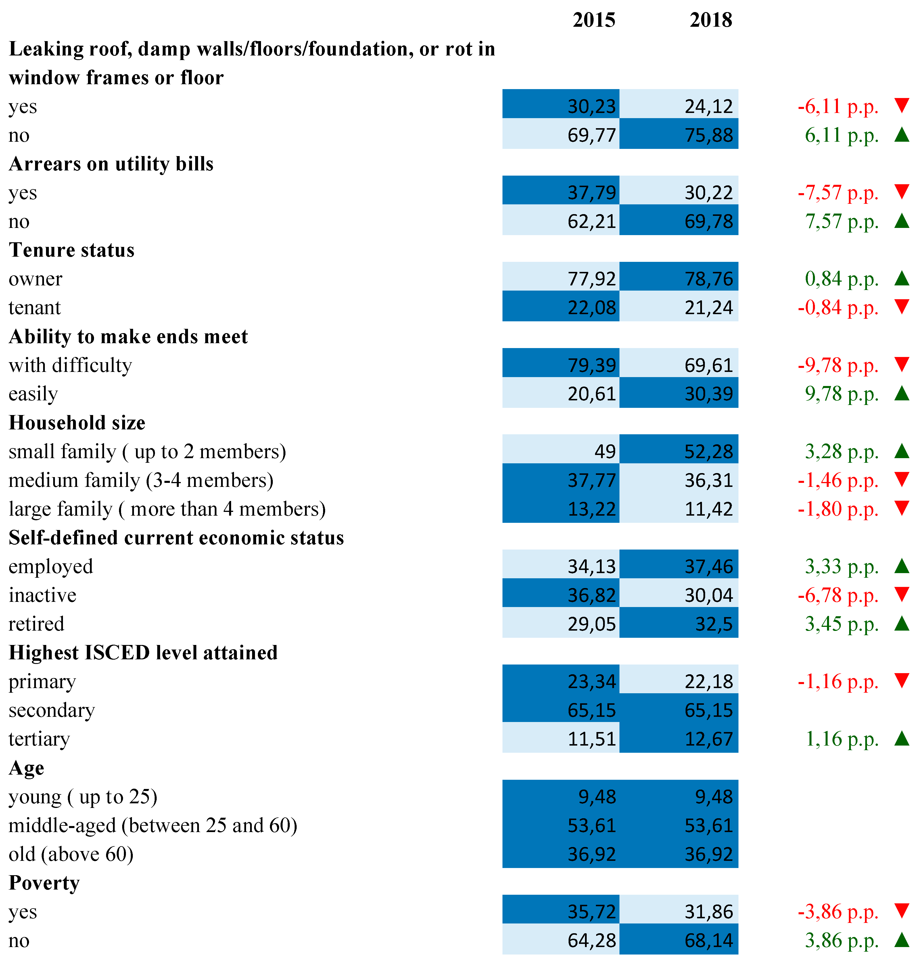
Figure 1 shows the frequency distribution of categorical variables for 10,150 households classified as energy poor in 2015. Statistics for the first and the last survey period are compared, the difference measured in percentage points is provided in the last column. In the heatmap, the more intense color corresponds to the highest frequency values. The share of households that have leaks/damp/and rot in a dwelling, arrears on utility bills, difficulties with making ends meet, and are income poor in 2015 decreases in 2018. Those households are mostly represented by medium-sized families with middle-aged members with secondary education. Surprisingly, the majority of energy-poor households are not classified as the poor in terms of their income. The share of owners is quite high, whereas the economic status is almost equally distributed among employed, professionally inactive, and retired people.
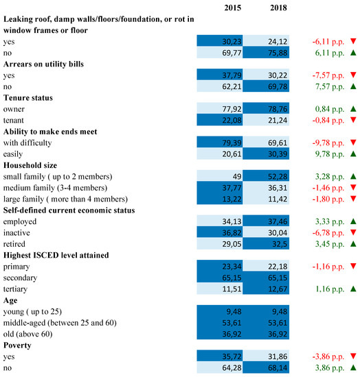
Figure 1.
Heatmap of the frequency distribution of variables (in percentage).
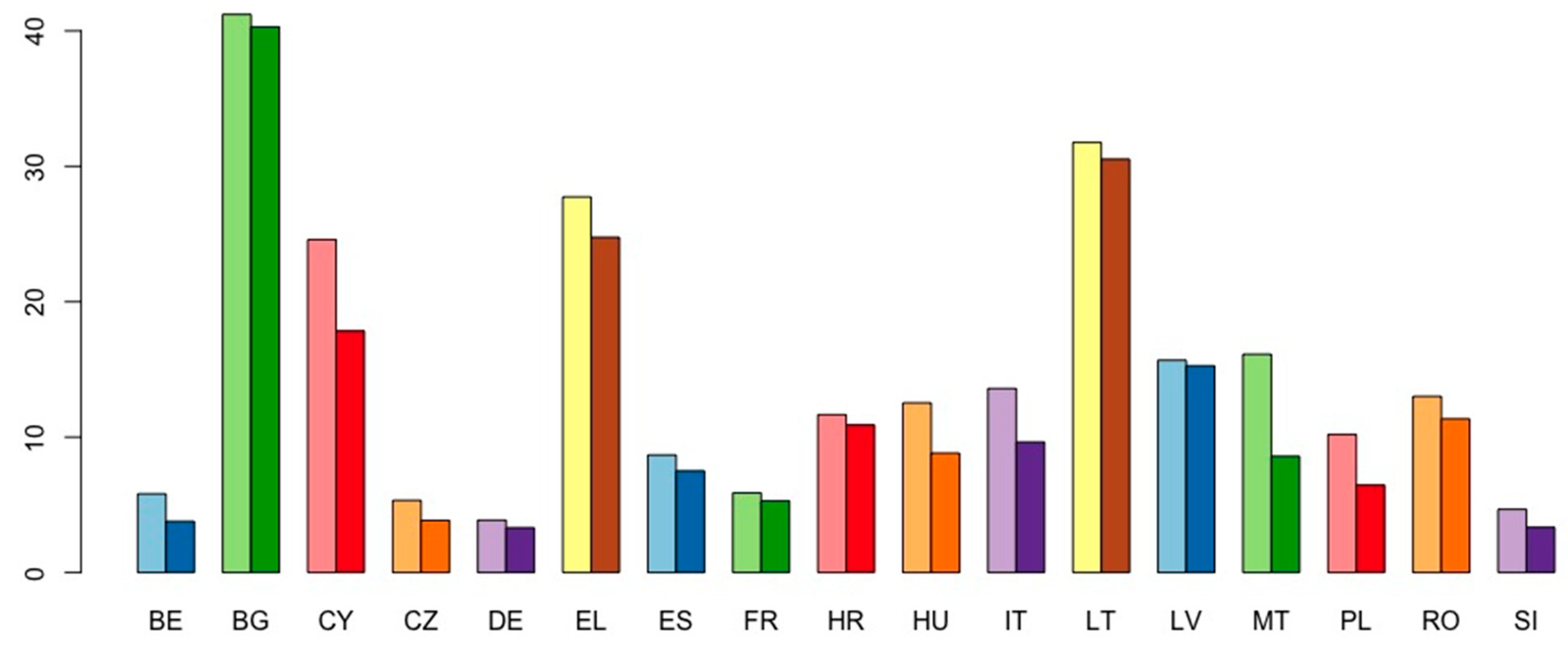
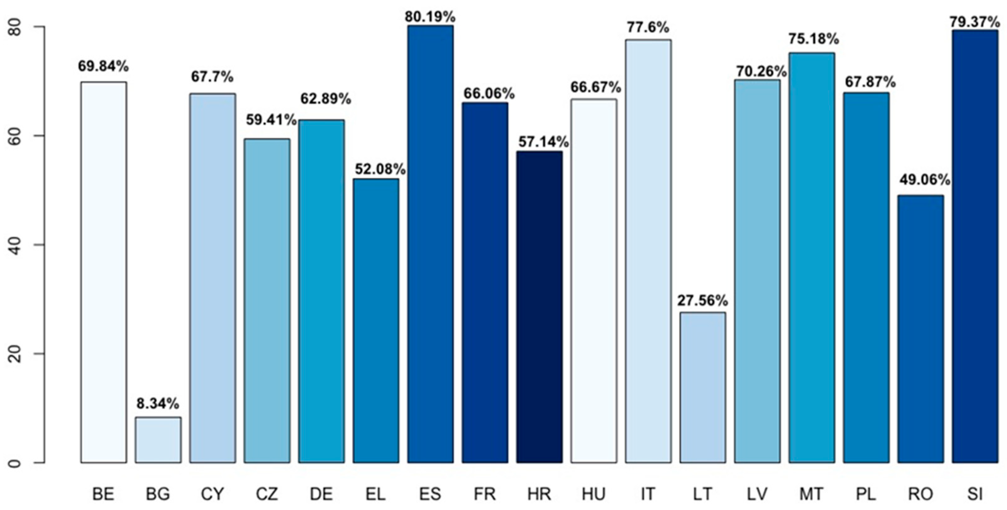
The energy poverty rate is computed based on the ability-to-keep-home-warm indicator. As depicted in Figure 2, Bulgaria, Latvia, and Greece have the highest incidence of energy poverty. By contrast, Germany, Slovenia, and Czechia have the lowest energy poverty rate. Figure 3 shows the energy poverty escape rate. The escape rate is calculated as a share of households that are energy poor in the first wave, but move out of energy poverty in the last wave. The high escape rate signifies the instability of the phenomenon in the period of four years. The highest value is noted in Spain and the lowest in Bulgaria.

Figure 2.
Energy poverty rate, values in 2015 and 2018 (in percentage).

Figure 3.
Energy poverty escape rate.
Table 1 contains descriptive statistics of the energy poverty rate and energy poverty escape rate for all 17 countries. Overall, the rate of energy poverty decreases in 2018 compared to 2015. The high standard deviation of the energy poverty escape rate indicates that the values are less concentrated around the mean.

Table 1.
Descriptive statistics for 17 countries.
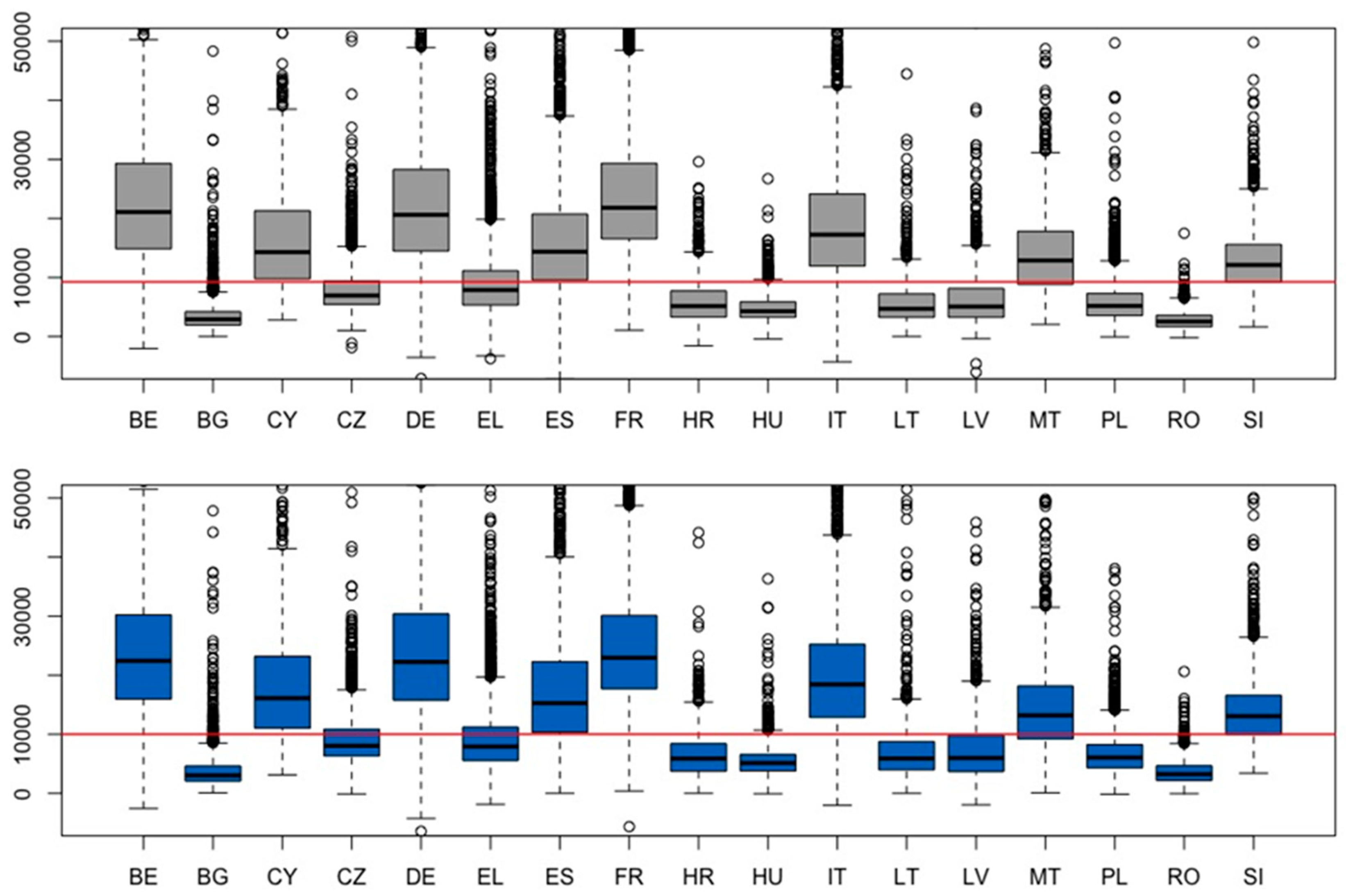
Our set of variables contains one continuous variable, i.e., equivalized disposable income. We use this variable to compute the poverty threshold, which is 60% of a national median equivalized disposable income. The respective boxplot distribution of equivalized disposable income in 2015 and 2018 is presented in Figure 4. There are no significant changes in income distribution in 2015 and 2018. Two groups of countries, the ones with low and high income, can be easily identified. The median value slightly increases from 9262.22 euros in 2015 to 10,008 euros in 2018. As mentioned above, only a small group of the energy-poor households, i.e., 35.72% in 2015 and 31.86% in 2018, are considered poor according to the standard poverty measure. This fact could be attributed to the discrepancy of classifications produced by subjective and objective indicators. In this study, poverty is included in the model as a determinant of escaping energy poverty.

Figure 4.
Boxplot distribution of annual equivalized disposable income in 2015 (upper panel) and 2018 (lower panel) and Europe-17 median values, in EUR.
4. Methodology
This study examines the patterns of transition in and out of energy poverty in 17 European countries and identifies the determinants of escaping energy poverty within four years. The study is conducted in two parts; each part corresponds to the research questions raised in the introduction. We propose a discrete-time Markov chain (DTMC) model to analyze the transition probabilities at a specific point in time. The Markov process is a tool recommended for studying poverty [36] and labor mobility [37]. Ref. [23] applies the mover-stayer extension of the Markov process in energy poverty analysis. This part is performed with R using a Markov chain package by Spedicato and Signorelli [38].
We also consider the binomial mixed effect model to identify events that trigger energy poverty escapes in all 17 countries and to account for a country-specific effect. Our sample consists of energy poor households from different countries and has a clear hierarchical structure. To account for a grouping factor, a number of authors recommend to rely on mixed effect models [39,40]. Additionally, this study relies on a hierarchical clustering technique that allows classifying countries with regard to transition probability patterns. In this part, we rely on the lme4 package by [41] and the cluster package [42] in R. Our choice of tools is partially based on the suggested techniques for longitudinal data analysis [36].
4.1. Markov Chain Model
The analysis draws on a multi-state stochastic model. The Markov process, with some modifications, is used in similar energy poverty analysis [23]. We specify a DTMC model as follows:
where X1, X2…Xn is a stochastic process of moving across states i and j after the elapse of a discrete-time (n). We consider two energy poverty classes, S = {S1 = energy poor, S2 = non-energy poor} and define a transition matrix:
where each row sums up to 1. In our model, we rely on two assumptions intrinsic to a Markov process. The first assumption is that the conditional probability is independent of the past (Markov property), i.e., we could predict the probability of transitions based on the information of the present state. The second assumption is that statistical units of the analysis, i.e., households in our case, are homogeneous [43], meaning that all observations are moving between states according to the same algorithm. To account for the differences in transition paths between various countries we build several DTMC models. The groups of countries are obtained in a hierarchical clustering procedure. Hierarchical clustering belongs to unsupervised learning methods, in which a bottom-up approach to group observations is used. To obtain clusters, different measures of distance between observations can be considered. In our study, we rely on Ward’s minimum variance criterion that minimizes the total variance within clusters. The results of the hierarchical clustering are usually presented in a dendrogram. The impact of households’ and countries’ characteristics is considered in the latter part of the analyses.
4.2. Binomial Mixed Effect Model
To estimate the chance of escaping from energy poverty we consider the regression function:
where is the latent variable which represents the observed binary categories: staying (0) or exiting (1) energy poverty; is the vector of predictors which includes the characteristics of houses and families; is the vector of the respective coefficient; is an error term. The subscripts i and j denote a household and a country, respectively.
Since the data have a hierarchical structure, the error term contains both the information on individual households and the country’s effects. As a result,
where represents countries and denotes household heterogeneity. It is assumed that both terms are uncorrelated, which implies that
We assume that is randomly distributed and might include country-specific factors. Consequently, model (3) has a random intercept that represents the variation among the countries.
5. Results and Discussion
First, we estimate the transition probabilities of moving out and into, as well as staying in, energy poverty and non-energy poverty states in each country. The results are presented in Table 2. A one-step transition probability matrix is a collection of all probabilities in a single step. The persistence of energy poverty can be assessed by the respective retention rate, i.e., the rate of returning to the same condition in the observed period. Additionally, the transitioning to energy poverty should be taken into account. The average energy poverty retention rate in all selected countries is more than 51%; the average probability of entering energy poverty is 5.4%. Statistics demonstrate that there are slightly more chances to remain in energy poverty than to escape it. Although, the average probability of transitioning to non-energy poverty is almost 9 times higher compared to the probability of moving to energy poverty, yet the high retention rate signifies problems households have with escaping energy poverty within four years.
Table 2.
One-step transition probability matrices for 17 countries.
The maximum value of the energy poverty retention rate is noted in Bulgaria (97%) and the minimum in Slovenia (25%). The results point to striking differences between European countries. In some countries, energy poverty seems to be unstable in the long run, whereas in others it is very difficult to escape energy poverty. In line with [23], we indicate that French households have a higher probability to leave energy poverty than to stay in it. Our results differ from the conclusions drawn by [22], who claim that the state of energy poverty in Spain measured by a subjective indicator is more pervasive. According to our results, and in comparison to other countries of Europe, Spain is better off in terms of energy poverty persistence. A possible difference results from the measurement technique used and the data span which—in the case of [22]—is close to the global financial crisis period that might have an impact on the ubiquity of energy poverty. The distribution of transition probability is an interesting point to consider in discussing the long-term policy effects.
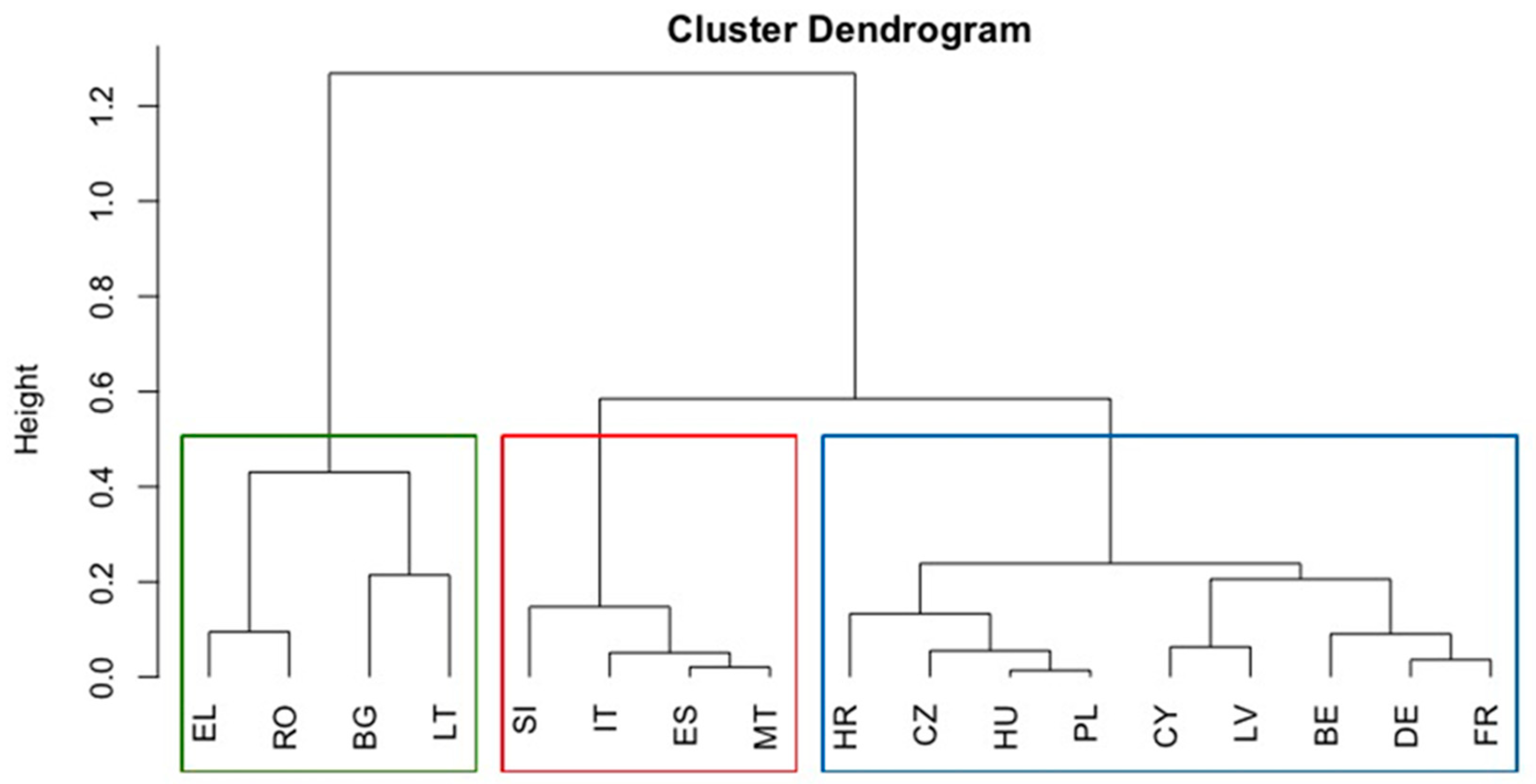
Transition paths in groups of countries show some similarities. Based on Table 2, we group countries minimizing the total within-cluster variance. As demonstrated in Figure 5, 3 distinct groups are identified. The first group consists of 9 countries (Belgium, Croatia, Cyprus, Czechia, France, Germany, Hungary, Latvia, Poland), while the second (Bulgaria, Greece, Lithuania, Romania) and the third (Italy, Spain, Malta, Slovenia) of 4 countries each. The results are robust to alternative k-means clustering technique (Figure A1). The suggested optimal number of clusters is 3–4. The same groups are obtained in 3-cluster partitioning.
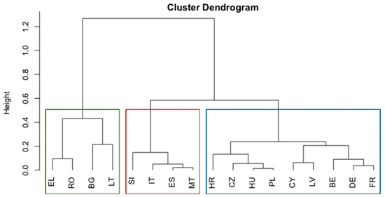
Figure 5.
Clustering based on transition probability matrices.
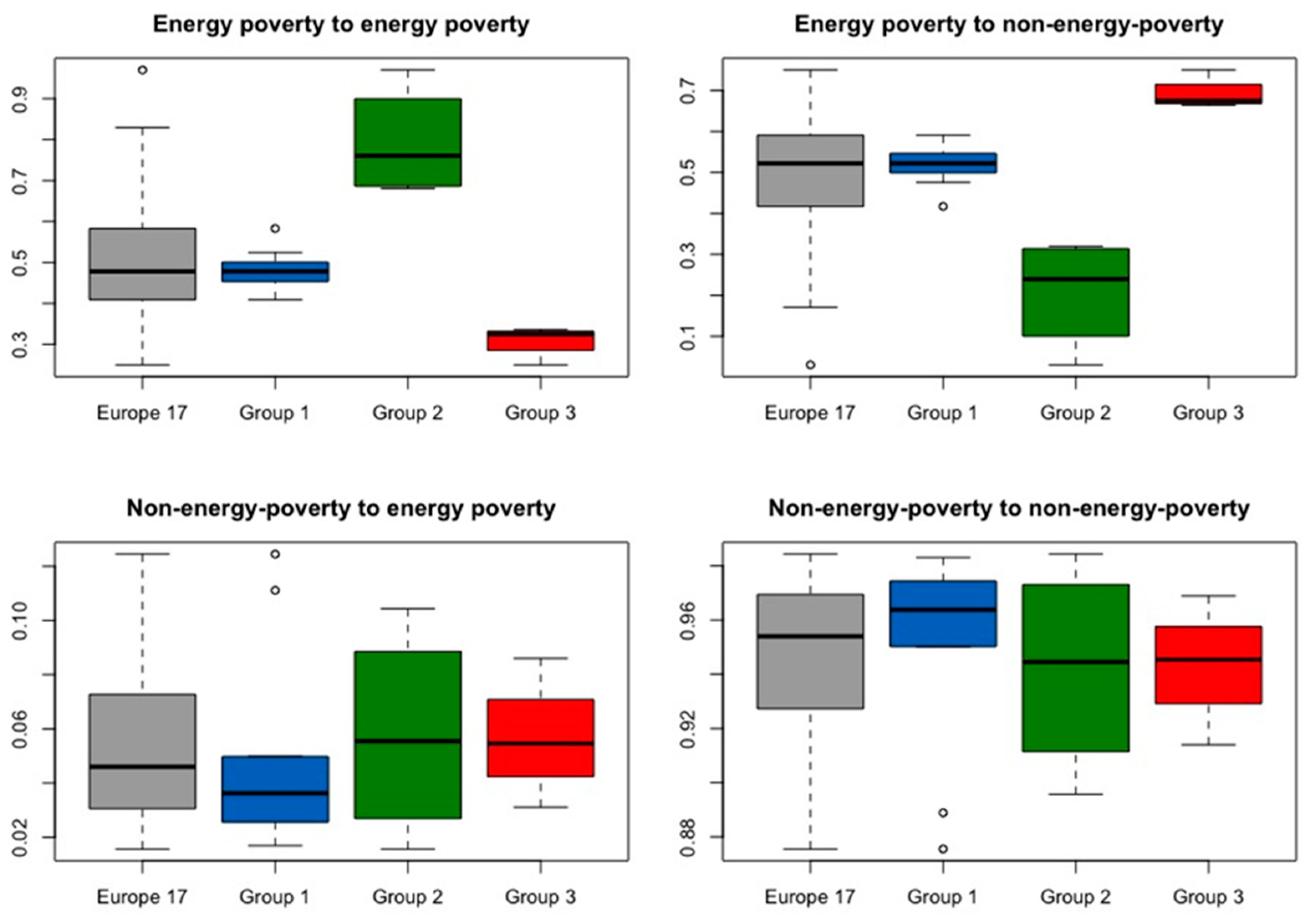
Figure 6 presents the distribution of transition probabilities in each group and all 17 countries. The results obtained in Group 1 are close to Europe-17. Several outliers are identified in this group, such as Croatia, in which the energy poverty retention rate is 58.3%, and Cyprus and Lithuania, in which the chances to transit into energy poverty are high, i.e., 12.4% and 11.1%, respectively. Group 1 is also characterized by small overall dispersion, which means that member countries of this group share a lot of similarities in terms of their transition probability. Groups 2 and 3 have rather dissimilar distributions, especially the ones concerning energy poverty transitions. We could say that in Group 2 energy poverty appears to be more persistent. Furthermore, there is high variability in non-energy poverty probabilities among countries from Group 2, as shown by the interquartile range. Countries in Group 3 are better off in terms of energy poverty persistence. By contrast, movements from non-energy poverty to energy poverty are more intensive in Group 3 than in Group 1.

Figure 6.
Distribution of transition probabilities in groups of countries.
Second, we examine the determinants of escaping energy poverty in a four-year time perspective by building a binomial mixed effect model. In this part, our sample is limited to household members that declare problems with keeping the home warm in the base year 2015. Our response variable indicates successful energy poverty escape if a household changes its status from unable to keep the home warm in 2015 to able to keep the home warm in 2018. Factors that have an impact on escaping energy poverty are included in the model, and we also construct several “happy” scenario variables that indicate positive changes happening to household members in 2018. Positive changes are associated with getting income, i.e., the change of economic status from being inactive to active or retired, with renovation, i.e., having no leaks/damp/rot, and with being able to make ends meet and settle arrears on utility bills in 2018 compared to 2015. Variables indicating favorable changes are frequently used in modeling poverty dynamics [44,45].
The results of the mixed-effect regression are presented in Table 3. The overwhelming majority of fixed effect variables are very significant. The age variable is a rare exception. We observe that good (with no leaks/damp/rot) or renovated buildings, tertiary and even secondary education, owner tenure status, living in a large family, and employment significantly increase the probability of exiting energy poverty. Tenants have limited possibilities to invest in house renovation compared to owners. By sharing a house, large families can save on energy costs. Poverty, measured by either income-based or subjective indicators, impedes the ability to escape energy poverty. Young age is positively associated with the ability to get out of energy poverty. The results also reveal the high significance of positive changes, particularly of the ability to make ends meet. Our study supports the evidence provided by [21], that one-person households and old age, among others, decrease the probability to move out of energy poverty. In addition, the strong impact of house renovation and employment on the ability to leave energy poverty is also confirmed by [23]. In our model, the status of a tenant impedes energy poverty escapes. As reported in the literature, rented housing is usually associated with energy poverty and a wide range of structural disadvantages [46].
Table 3.
The results of the mixed effect model.
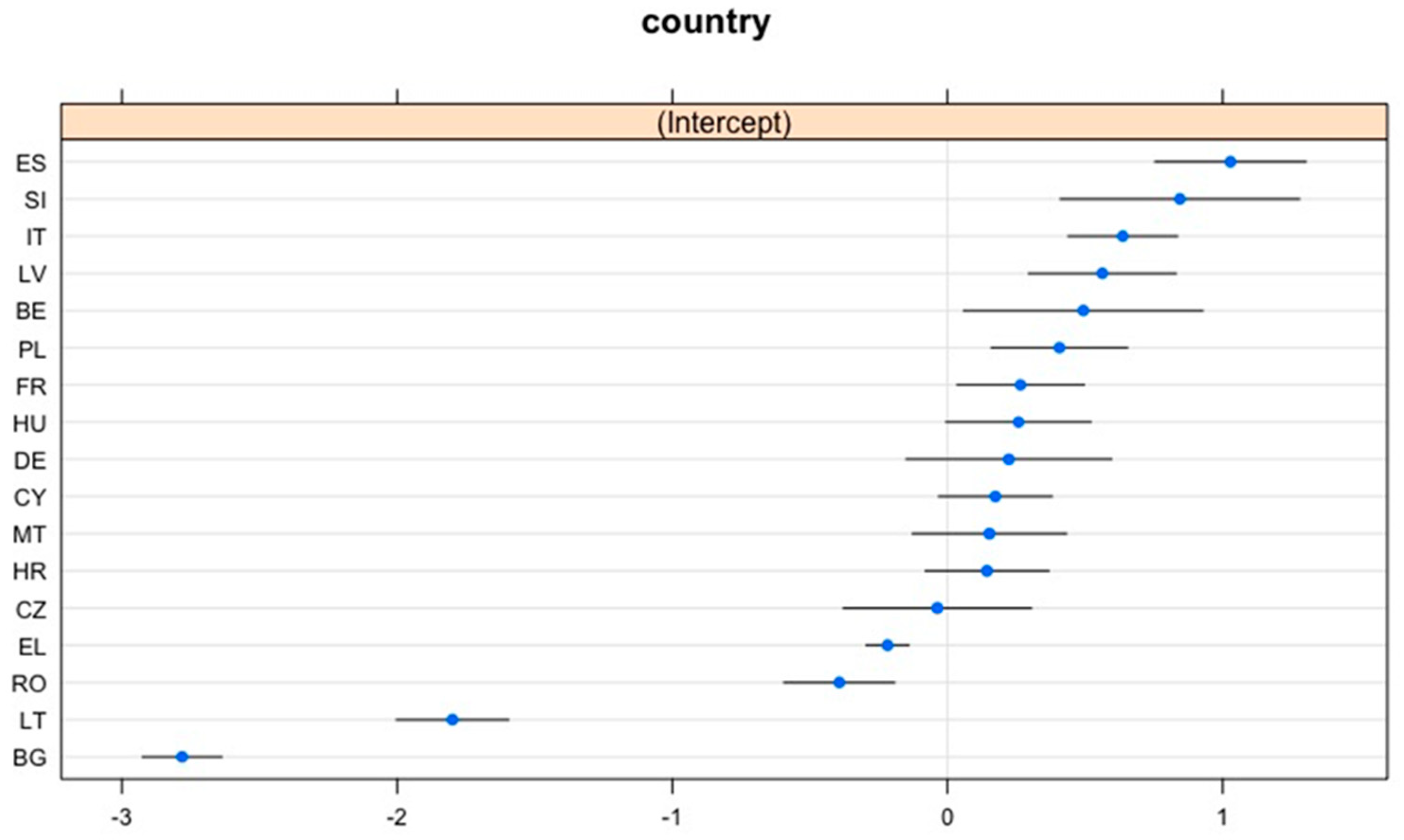
Figure 7 shows the distribution of varying intercepts across countries, which is a grouping factor in our model. Consequently, 17 conditional modes of the random effect are extracted from the model. In general, the distribution of intercepts corresponds to the hierarchical clustering results conducted on the basis of transition probability paths. While the majority of countries have a positive value of the intercept, some countries, such as Bulgaria, Lithuania, Romania, and Greece, stand out. The among-countries standard deviation of the intercept is 0.93. To test the significance of the country’s random effect, we use the likelihood-ratio test of the full model (model 2) and the reduced model (model 1), i.e., the model without country variable. Table 4 shows that adding country random effect results in a much better model.
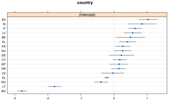
Figure 7.
Random effects plot.
Table 4.
ANOVA test of the country’s random effect significance.
The country’s random effect could be attributed to geographical factors, such as climate, a level of socio-economic development, and a degree of urbanization, which play a non-negligible role in energy poverty persistence [20].
Not all 17 countries contain variables that might be useful for the analysis. To estimate the significance of some missing variables, such as regions (DB040), degree of urbanization (DB100), dwelling type (HH010), year of contract or purchasing or installation (HH031), and a number of rooms (HH030), we include these variables and shrink the number of countries in a dataset to 14. We exclude Germany, Slovenia, and Latvia, reducing the total number of observations by 5.6%. The new dataset consists of 9573 households. The results of the mixed model for 14 countries are presented in Table A1. The second mixed effect model has two grouping factors, i.e., country and region. Except for the new installation, the added variables carry small or negligible significance. The among-regions standard deviation of the intercept is 0.49. We apply the same test of the random effect significance. This time, we exclude the region variable from the reduced model. The ANOVA output provides evidence that including regions would significantly improve the model (Table A2). However, we should account for the low representation in the vast majority of regions, which might distort the results. In light of the above arguments, we conclude that the initial set of countries and variables provides a good fit to the model.
6. Conclusions
This study focuses on the persistence of energy poverty in 17 European countries by considering the transition probability paths of households in each country. We rely on the latest available longitudinal data from the EU-SILC, waves 2015–2018, and use the subjective energy poverty indicator, which is the ability to keep homes warm. This indicator allows for applying a uniform approach to measuring energy poverty in countries having different socio-economic environments. The subjective energy poverty measure does not require additional assumptions or thresholds tuning. The persistence of energy poverty is understood as a probability of staying in the same condition in 4 years. Following the DTMC process, we discover three groups of countries that have similar patterns of moving in and out of two states: energy poverty and non-energy poverty. The grouping results are robust to alternative k-means clustering.
The analysis helps to understand the dynamics of energy poverty in 17 countries. The results suggest that households in some countries face serious problems in transitioning from energy poverty. For example, in a group of Bulgaria, Greece, Lithuania, and Romania, we observe the highest energy poverty retention rate compared to other groups. On average, the chances to remain in energy poverty in this group equal 80%, which signifies that the situation is close to the energy poverty trap. By contrast, in the group of Italy, Malta, Spain, and Slovenia, the average probability of moving out of energy poverty (31%) is the lowest among all groups. The average retention rate of energy poverty in the remaining countries (48.4%) is close to the European average results (51.5%). The high value of the interquartile range of the energy poverty retention rate (72%) points to a great disparity between countries in terms of energy poverty persistence. The lack of cohesion within the European countries and a clear division into groups should be further considered in the European region and energy poverty policy.
The study also examines the factors that trigger energy poverty exits in a 4-year time perspective in households classified as energy poor at the beginning of the observation period. This part of the analysis is based on a dataset consisting of 10150 observations from all countries. Regression results from the mixed effect model reveal a strong effect of the among-country varying intercept. The determinants of escaping energy poverty include, e.g., housing conditions, poverty, employment, education, and tenure status. Most variables have a high significance. Young age, ability to make ends meet, and higher education are positively associated with the chances to exit energy poverty. Poverty and renovation of the building are the positive changes that exert the greatest impact on the chances to escape energy poverty. Policy makers may consider the key determinants of escaping energy poverty in formulating policies aimed at energy poverty alleviation.
We would like to convey several messages to policy makers. First, the level of energy poverty computed for each country should be accompanied by persistence analysis. In a four-year period, in many countries energy poverty is not a stable state, whereas in others the situation is almost a trap. The persistence of energy poverty determines policy mechanisms. Second, we suggest relying more on short-term policy actions and preventive measures in countries where energy poverty is less persistent. For example, short-term actions might include houses renovation and raising public awareness, etc. In countries where energy poverty is hard to escape, long-term strategies and complex policies improving socio-economic situation, i.e., employment and taxation, should be a priority. Short- and long-term policies should be combined in both cases. Third, the regional disparity between European countries point to a lack of cohesion within the EU. Some countries, such as Greece, Bulgaria, Lithuania, and Bulgaria, are much worse off when it comes to the persistence of energy poverty. EU regional policy is one of the instruments suitable to tackle the issue. Fourth, we identify the determinants of energy poverty escapes common to energy-poor households from all analyzed countries. Demographic, technical, and socio-economic factors are the drivers in escaping energy poverty, which suggests common EU policy. EU-wide policies aimed to improve these factors can be effective in combating energy poverty in all countries. Fifth, the dynamics of energy poverty should be monitored on a regular basis as it offers a valuable insight into the effectiveness of the respective policies and provides a forward-looking policy perspective.
The limitation of this analysis is related to the availability of data. Although the EU-SILC is harmonized across many European countries, there are differences in datasets. In order to conduct the mixed-effect regression analysis, we have to select countries that contain more than one hundred energy-poor households in the initial period, which also limits the number of countries. Further studies on this topic may include the analysis of energy poverty profiles and the determinants of escaping energy poverty in each country.
Author Contributions
Conceptualization, L.K. and S.Ś.; methodology, L.K. and S.Ś.; software, L.K. and S.Ś.; validation, L.K. and S.Ś.; investigation, L.K. and S.Ś.; data curation, L.K.; writing—original draft preparation, L.K.; writing—review and editing, L.K. and S.Ś.; visualization, L.K. and S.Ś.; supervision, S.Ś.; project administration, S.Ś.; funding acquisition, S.Ś. All authors have read and agreed to the published version of the manuscript.
Funding
The Research Excellence Program in Cracow University of Economics, grant no. 64/EIT/2021/DOS.
Institutional Review Board Statement
Not applicable.
Informed Consent Statement
Not applicable.
Data Availability Statement
Not applicable.
Acknowledgments
The access to the EU-SILC micro-data was granted by Eurostat within the framework of the Research Project Proposal 204/2018-EU-SILC. The publication was financed from the Research Excellence Program and allocated from the subvention granted to Cracow University of Economics, grant no. 64/EIT/2021/DOS.
Conflicts of Interest
The authors declare no conflict of interest.
Appendix A

Figure A1.
Random effect K-means goodness of classification plots: elbow (left panel) and silhouette (right panel).
Figure A1.
Random effect K-means goodness of classification plots: elbow (left panel) and silhouette (right panel).
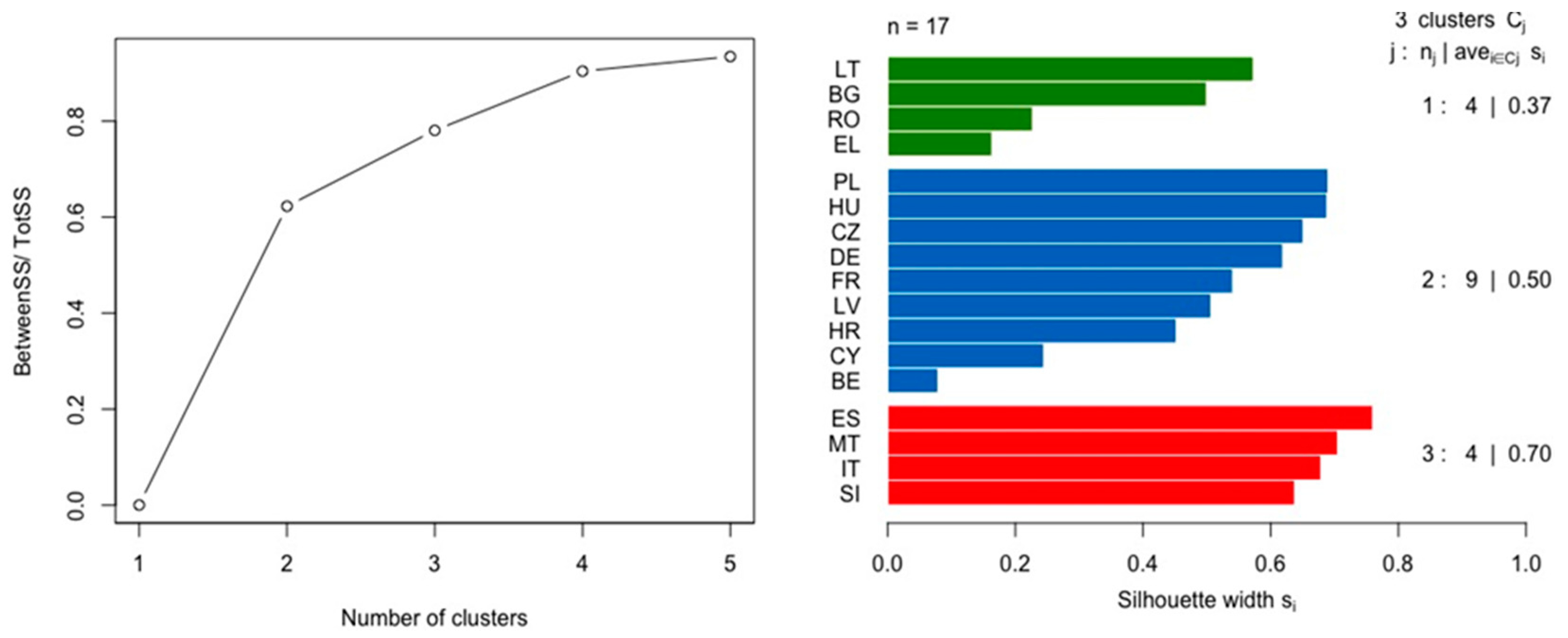
Table A1.
The results of the mixed effect model for 14 countries (with additional variables).
Table A1.
The results of the mixed effect model for 14 countries (with additional variables).
| Fixed Effects Coefficients: | Estimate | Std. Error | z Value | Pr (>|z|) | |
|---|---|---|---|---|---|
| (Intercept) | −0.434 | 0.300 | −1.449 | 0.147 | |
| Leaks/damp/rot: no leaks/damp/rot | 0.497 | 0.073 | 6.824 | 0.000 | *** |
| Tenure status: tenant | −0.306 | 0.067 | −4.541 | 0.000 | *** |
| Poverty: poor | −0.348 | 0.059 | −5.941 | 0.000 | *** |
| Ability to make ends meet: easily | 0.768 | 0.074 | 10.370 | 0.000 | *** |
| Age: middle-aged | −0.080 | 0.087 | −0.928 | 0.353 | |
| Age: young | −0.013 | 0.120 | −0.109 | 0.914 | |
| Household size: medium family | 0.352 | 0.063 | 5.636 | 0.000 | *** |
| Household size: large family | 0.375 | 0.090 | 4.159 | 0.000 | *** |
| Education: secondary | 0.164 | 0.070 | 2.332 | 0.020 | * |
| Education: tertiary | 0.421 | 0.104 | 4.062 | 0.000 | *** |
| Economic status: inactive | −0.354 | 0.071 | −4.961 | 0.000 | *** |
| Economic status: retired | −0.212 | 0.095 | −2.224 | 0.026 | * |
| Degree of urbanization: intermediate area | −0.091 | 0.074 | −1.234 | 0.217 | |
| Degree of urbanization: thinly populated area | 0.159 | 0.078 | 2.046 | 0.041 | * |
| Dwelling type: blocks of flats | 0.014 | 0.069 | 0.197 | 0.844 | |
| Number of rooms: up to 4 rooms | −0.119 | 0.070 | −1.703 | 0.089 | . |
| Number of rooms: more than 4 rooms | −0.021 | 0.079 | −0.271 | 0.787 | |
| Positive changes: become active/retired | 0.408 | 0.093 | 4.395 | 0.000 | *** |
| Positive changes: renovation | 0.818 | 0.097 | 8.394 | 0.000 | *** |
| Positive changes: able to make ends meet | 1.784 | 0.091 | 19.635 | 0.000 | *** |
| Positive changes: settle arrears on utility bills | 0.509 | 0.072 | 7.018 | 0.000 | *** |
| Positive changes: new installation | 0.333 | 0.077 | 4.317 | 0.000 | *** |
| Random effects: | Variance | SD | |||
| region (Intercept) | 0.2489 | 0.4989 | |||
| country (Intercept) | 0.8714 | 0.9335 | |||
Notes: Significance codes: 0 ‘***’ 0.001 ‘**’ 0.01 ‘*’ 0.05 ‘.’ 0.1 ‘ ’. Goodness of fit: AIC 9560.2; BIC 9739.3.
Table A2.
ANOVA test of the region’s random effect significance.
Table A2.
ANOVA test of the region’s random effect significance.
| Model | Parameters | AIC | BIC | Log-Likelihood | Deviance | Chisq | D | Pr (>Chisq) |
|---|---|---|---|---|---|---|---|---|
| 1 | 24 | 9687.4 | 9859.4 | −4819.7 | 9639.4 | |||
| 2 | 25 | 9560.2 | 9739.3 | −4755.1 | 9510.2 | 129.24 | 1 | 0.000 *** |
Notes: Significance codes: 0 ‘***’ 0.001 ‘**’ 0.01 ‘*’ 0.05 ‘.’ 0.1 ‘ ’.
References
- Bouzarovski, S.; Thomson, H.; Cornelis, M. Confronting Energy Poverty in Europe: A Research and Policy Agenda. Energies 2021, 14, 858. [Google Scholar] [CrossRef]
- Recalde, M.; Peralta, A.; Oliveras, L.; Tirado-Herrero, S.; Borrell, C.; Palència, L.; Gotsens, M.; Artazcoz, L.; Marí-Dell’Olmo, M. Structural energy poverty vulnerability and excess winter mortality in the European Union: Exploring the association between structural determinants and health. Energy Policy 2019, 133, 110869. [Google Scholar] [CrossRef]
- Betto, F.; Garengo, P.; Lorenzoni, A. A new measure of Italian hidden energy poverty. Energy Policy 2020, 138, 111237. [Google Scholar] [CrossRef]
- Castaño-Rosa, R.; Solís-Guzmán, J.; Marrero, M. Energy poverty goes south? Understanding the costs of energy poverty with the index of vulnerable homes in Spain. Energy Res. Soc. Sci. 2020, 60, 101325. [Google Scholar] [CrossRef]
- Papada, L.; Kaliampakos, D. Being forced to skimp on energy needs: A new look at energy poverty in Greece. Energy Res. Soc. Sci. 2020, 64, 101450. [Google Scholar] [CrossRef]
- Thomson, H.; Snell, C. Quantifying the prevalence of fuel poverty across the European Union. Energy Policy 2013, 52, 563–572. [Google Scholar] [CrossRef]
- Deller, D. Energy affordability in the EU: The risks of metric driven policies. Energy Policy 2018, 119, 168–182. [Google Scholar] [CrossRef] [Green Version]
- Bouzarovski, S.; Herrero, S.T. The energy divide: Integrating energy transitions, regional inequalities and poverty trends in the European Union. Eur. Urban Reg. Stud. 2017, 24, 69–86. [Google Scholar] [CrossRef] [Green Version]
- Chaudhuri, S. Assessing Vulnerability to Poverty: Concepts, Empirical Methods and Illustrative Examples; Department of Economics, Columbia University: New York, NY, USA, 2003; Volume 56. [Google Scholar]
- Thema, J.; Vondung, F. EPOV Indicator Dashboard: Methodology Guidebook; Wuppertal Institut für Klima, Umwelt, Energie GmbH: Wuppertal, Germany, 2020. [Google Scholar]
- Rademaekers, K.; Yearwood, J.; Ferreira, A.; Pye, S.; Hamilton, I.; Agnolucci, P.; Grover, D.; Karásek, J.; Anisimova, N. Selecting Indicators to Measure Energy Poverty—Under the Pilot Project ‘Energy Poverty—Assessment of the Impact of the Crisis and Review of Existing and Possible New Measures in the Member States. Framew. Contract ENER A 2016, 4, 1–130. [Google Scholar]
- Price, C.W.; Brazier, K.; Wang, W. Objective and subjective measures of fuel poverty. Energy Policy 2012, 49, 33–39. [Google Scholar] [CrossRef]
- Healy, J.D.; Clinch, J.P. Fuel poverty in Europe: A cross-country analysis using a new composite measurement. In Environmental Studies Research Series Working Papers; University College Dublin: Dublin, Ireland, 2002. [Google Scholar]
- Hills, J. Getting the Measure of Fuel Poverty Final Report of the Fuel Poverty Review; London School of Economics and Political Science: London, UK, 2012. [Google Scholar]
- Jahedi, S.; Méndez, F. On the advantages and disadvantages of subjective measures. J. Econ. Behav. Organ. 2014, 98, 97–114. [Google Scholar] [CrossRef]
- Sokołowski, J.; Lewandowski, P.; Kiełczewska, A.; Bouzarovski, S. A multidimensional index to measure energy poverty: The Polish case. Energy Sources Part B Econ. Plan. Policy 2020, 15, 92–112. [Google Scholar] [CrossRef]
- Karpinska, L.; Śmiech, S. Breaking the cycle of energy poverty. Will Poland make it? Energy Econ. 2021, 94, 105063. [Google Scholar] [CrossRef]
- Dubois, U.; Meier, H. Energy affordability and energy inequality in Europe: Implications for policymaking. Energy Res. Soc. Sci. 2016, 18, 21–35. [Google Scholar] [CrossRef]
- Arsenopoulos, A.; Marinakis, V.; Koasidis, K.; Stavrakaki, A.; Psarras, J. Assessing Resilience to Energy Poverty in Europe through a Multi-Criteria Analysis Framework. Sustainability 2020, 12, 4899. [Google Scholar] [CrossRef]
- Roberts, D.; Vera-Toscano, E.; Phimister, E. Fuel poverty in the UK: Is there a difference between rural and urban areas? Energy Policy 2015, 87, 216–223. [Google Scholar] [CrossRef] [Green Version]
- Kearns, A.; Whitley, E.; Curl, A. Occupant behaviour as a fourth driver of fuel poverty (aka warmth & energy deprivation). Energy Policy 2019, 129, 1143–1155. [Google Scholar]
- Phimister, E.; Vera-Toscano, E.; Roberts, D. The dynamics of energy poverty: Evidence from Spain. Econ. Energy Environ. Policy 2015, 4, 153–166. [Google Scholar] [CrossRef] [Green Version]
- Chaton, C.; Lacroix, E. Does France have a fuel poverty trap? Energy Policy 2018, 113, 258–268. [Google Scholar] [CrossRef]
- Churchill, S.A.; Smyth, R.; Farrell, L. Fuel poverty and subjective wellbeing. Energy Econ. 2020, 86, 104650. [Google Scholar] [CrossRef]
- Baudu, R.; Charlier, D.; Legendre, B. Fuel Poverty and Health: A Panel Data Analysis. FAERE Work. Pap. 2020, 4, 2274–5556. [Google Scholar]
- Churchill, S.A.; Smyth, R. Energy poverty and health: Panel data evidence from Australia. Energy Econ. 2021, 97, 105219. [Google Scholar] [CrossRef]
- Alem, Y.; Demeke, E. The persistence of energy poverty: A dynamic probit analysis. Energy Econ. 2020, 90, 104789. [Google Scholar] [CrossRef]
- Kahouli, S. An economic approach to the study of the relationship between housing hazards and health: The case of residential fuel poverty in France. Energy Econ. 2020, 85, 104592. [Google Scholar] [CrossRef]
- Karpinska, L.; Śmiech, S. On the Persistence of Energy Poverty in Europe: How Hard Is It for the Poor to Escape? Energy Res. Lett. 2020, 1, 14158. [Google Scholar] [CrossRef] [PubMed]
- Belaïd, F. Exposure and risk to fuel poverty in France: Examining the extent of the fuel precariousness and its salient determinants. Energy Policy 2018, 114, 189–200. [Google Scholar] [CrossRef]
- Bouzarovski, S.; Herrero, S.T. Geographies of injustice: The socio-spatial determinants of energy poverty in Poland, the Czech Republic and Hungary. Post-Communist Econ. 2017, 29, 27–50. [Google Scholar] [CrossRef] [Green Version]
- Csoknyai, T.; Legardeur, J.; Akle, A.A.; Horváth, M. Analysis of energy consumption profiles in residential buildings and impact assessment of a serious game on occupants’ behavior. Energy Build. 2019, 196, 1–20. [Google Scholar] [CrossRef]
- Primc, K.; Slabe-Erker, R.; Majcen, B. Constructing energy poverty profiles for an effective energy policy. Energy Policy 2019, 128, 727–734. [Google Scholar] [CrossRef]
- Legendre, B.; Ricci, O. Measuring fuel poverty in France: Which households are the most fuel vulnerable? Energy Econ. 2015, 49, 620–628. [Google Scholar] [CrossRef] [Green Version]
- Karpinska, L.; Śmiech, S. Invisible energy poverty? Analysing housing costs in Central and Eastern Europe. Energy Res. Soc. Sci. 2020, 70, 101670. [Google Scholar] [CrossRef]
- Cappellari, L.; Jenkins, S.P. Who Stays Poor? Who Becomes Poor? Evidence From The British Household Panel Survey. Econ. J. 2002, 112, C60–C67. [Google Scholar] [CrossRef]
- Blumen, I.M.; Kogan, M.; McCarthy, P.J. The Industrial Mobility of Labor as a Probability Process; Cornell University Press: Ithaca, NY, USA, 1955. [Google Scholar]
- Spedicato, G.A.; Signorelli, M. The Markovchain Package: A Package for Easily Handling Discrete Markov Chains in R. 2014. Available online: https://cran.r-project.org/web/packages/markovchain/vignettes/an_introduction_to_markovchain_package.pdf (accessed on 4 August 2021).
- Raudenbush, S.W.; Bryk, A.S. Hierarchical Linear Models: Applications and Data Analysis Methods, 2nd ed.; Sage: Thousand Oaks, CA, USA, 2002. [Google Scholar]
- Goldstein, H. Multilevel Statistical Models; Wiley Series in Probability and Statistics; John Wiley & Sons, Ltd.: Chichester, UK, 2010. [Google Scholar] [CrossRef] [Green Version]
- Bates, D.; Mächler, M.; Bolker, B.; Walker, S. Fitting Linear Mixed-Effects Models Using lme4. J. Stat. Softw. 2015, 67, 1–48. [Google Scholar] [CrossRef]
- Maechler, M.; Rousseeuw, P.; Struyf, A.; Hubert, M.; Hornik, K. Cluster: Cluster Analysis Basics and Extensions; R Package Version; Eidgenössische: Zürich, Switzerland, 2012; Volume 1, p. 56. [Google Scholar]
- Singer, B.; Spilerman, S. Some Methodological Issues in the Analysis of Longitudinal Surveys. Soc. Demogr. 1978, 5, 261–296. [Google Scholar] [CrossRef] [Green Version]
- Duncan, G.J.; Gustafsson, B.; Hauser, R.; Schmauss, G.; Messinger, H.; Muffels, R.; Nolan, B.; Ray, J.-C. Poverty dynamics in eight countries. J. Popul. Econ. 1993, 6, 215–234. [Google Scholar] [CrossRef]
- Oxley, H.; Thai-Thanh, D.; Antolín, P. Poverty dynamics in six OECD countries. OECD Econ. Stud. 2000, 30, 7–52. [Google Scholar]
- Seebauer, S.; Friesenecker, M.; Eisfeld, K. Integrating climate and social housing policy to alleviate energy poverty: An analysis of targets and instruments in Austria. Energy Sources Part B Econ. Plan. Policy 2019, 14, 304–326. [Google Scholar] [CrossRef]
Publisher’s Note: MDPI stays neutral with regard to jurisdictional claims in published maps and institutional affiliations. |
© 2021 by the authors. Licensee MDPI, Basel, Switzerland. This article is an open access article distributed under the terms and conditions of the Creative Commons Attribution (CC BY) license (https://creativecommons.org/licenses/by/4.0/).