Abstract
The stability problem for load frequency control (LFC) of power systems with two time-varying communication delays is studied in this paper. The one-area and two-area LFC systems are considered, respectively, which are modeled as corresponding linear systems with additive time-varying delays. An improved stability criterion is proposed via a modified Lyapunov-Krasovskii functional (LKF) approach. Firstly, an augmented LKF consisting of delay-dependent matrices and some single-integral items containing time-varying delay information in two different delay subintervals is constructed, which makes full use of the coupling information between the system states and time-varying delays. Secondly, the novel negative definite inequality equivalent transformation lemma is used to transform the nonlinear inequality to the linear matrix inequality (LMI) equivalently, which can be easily solved by the MATLAB LMI-Toolbox. Finally, some numerical examples are presented to show the improvement of the proposed approach.
1. Introduction
In order to maintain the power grid frequency (an important index of power quality) fixed or within a small allowable range, a load frequency control (LFC) strategy is a common technique equipped in the power systems [1,2,3,4,5,6,7]. With the development and expansion of the power grid, a dedicated independent communication network has been unable to meet the operation of the power grid, although the small transmission delay in the dedicated independent communication network can be ignored [8]. At present, the LFC scheme receives sensor signals and outputs control signals through an open communication network with a mass of data and extensive information exchange. However, random delays and data packets will be introduced into the LFC scheme through the open communication network, which are not negligible and important [9]. These network factors result in the LFC system performance degradation and even instability. Literature [10] pointed out that even if there is a time delay less than 100 ms in the process of information measurement and control output, the transient excitation controller of a generator cannot achieve the control goal. Thus, it is necessary to study the influence of time-varying delays on the performance of the LFC system in an open communication network.
The network controlled LFC system involves the transmitting data between controller and plant. Therefore, there are two main cases of time-varying delays: on the one hand, only the communication time-varying delay from the control center to the governor is considered [11,12,13,14,15,16,17,18], where delay-dependent stability analysis and controller design are investigated by using single delay to model all time delays arising in communication channels. In fact, the time delays arising in the feedback measurement channel and those in the forward control channel may have different properties. It has more useful guidelines with considering the different properties. Thus, on the other hand, not only the communication time-varying delays from the control center to the governor but also from the sensor to the LFC center are considered simultaneously [19,20,21], where general delay-dependent stability analysis is studied by using additive time-varying delays to model two different time delays arising in communication channels. In this way, the stability problems of the LFC system with two transmission delays can be investigated by using the method of stability analysis for general linear time-delayed systems.
The main analytical purpose is obtaining the stability condition and controller design method via Lyapunov stability theory application. The stability criterion based on Lyapunov stability theory is a sufficient condition, and inevitably has certain conservativeness. There are two main reasons for the conservativeness: the construction of LKF and techniques for estimating the upper bound of the derivative of LKF. Thus, there are many methods and techniques given to address these two aspects. For the construction of LKF, a LKF with the delay decomposition method [22,23,24], LKF with multiple integral items [25,26,27,28,29] and LKF with some augmented vectors [30,31] are proposed. On the other aspect, the Jensen inequality [32], B-L inequality [33] and relaxed integral inequality techniques [34,35,36,37,38] are used to estimate the upper bound of the derivative of LKF. In order to reduce the conservativeness of the LKF construction, a lot of coupling information between the system state variables and time delays is introduced into the LKF, which leads to some nonlinear terms in the final results. This makes the solution complex and even unsolvable. Recently, a novel negative definite inequality equivalent transformation lemma was proposed in [39], which improved the degree of freedom for solving the linear matrix inequality (LMI) in the main theorem without conservativeness. Thus, according to the development of stability methods for linear time-delayed systems, there is still space to further reduce the conservativeness of stability criteria for the LFC system.
Inspired by the above analysis, the contributions of this paper can be summarized as follows:
- As mentioned above, only one-area LFC system with two different time-varying delays is considered. It is general and important to investigate the stability of two-area or multi-area LFC system with two or more time-varying delays. This paper studies one- and two-area LFC system with two time-varying delays.
- The main improvements of the LKF are summarized as: (a) introducing four delay-dependent non-integral terms to the LKF, such as , (i = 1, 2, 3, 4); (b) introducing some integral components to the single-integral terms under different time-varying delay subintervals, such as , , , , and so on. These improvements make the LKF contain more information (the time-varying delays and the coupling information between the state variables and the time-varying delay) than the literature [11,17,18,21], which reduces the conservativeness caused by the LKF construction.
- To overcome the nonlinear matrix inequality in the stability criterion, the novel negative definite inequality equivalent transformation lemma proposed in [39] is used to transform the nonlinear inequality to the LMI equivalently, which can be easily solved by the MATLAB LMI-Toolbox.
In this paper, the stability problem for LFC power systems with two time-varying communication delays is studied. Both one-area and two-area LFC systems are considered, respectively. An improved stability criterion is proposed via a modified LKF approach. Firstly, an augmented LKF consisting of delay-dependent matrices and some single-integral items containing time-varying delay information in two different delay subintervals is constructed. Secondly, a novel negative definite inequality equivalent transformation lemma is used to transform the nonlinear inequality to the LMI equivalently, which can be easily solved by the MATLAB LMI-Toolbox. Finally, some numerical examples are presented to show the improvement of the proposed approach. Moreover, the stability results can be applied to the LFC optimization to guarantee the stable operation of power system based on an open interconnect network control.
This paper is organized as follows. Section 2 gives the models of LFC schemes; Section 3 provides a stability assessment for the LFC system. Section 4 shows numerical examples. Conclusions are drawn in Section 5.
Notation 1.
Throughout this paper, the notations are standard. denotes the n-dimensional Euclidean space; is the set of all real matrices; For , (respectively, ) mean that P is a positive (respectively, negative) definite matrix. denotes an n-order diagonal matrix with diagonal elements . are block entry matrices. For example, . For a real matrix B and two real symmetric matrices A and C of appropriate dimensions, denotes a real symmetric matrix, where * denotes the entries implied by symmetry. .
2. System Description and Problem Preliminaries
2.1. One-Area LFC System
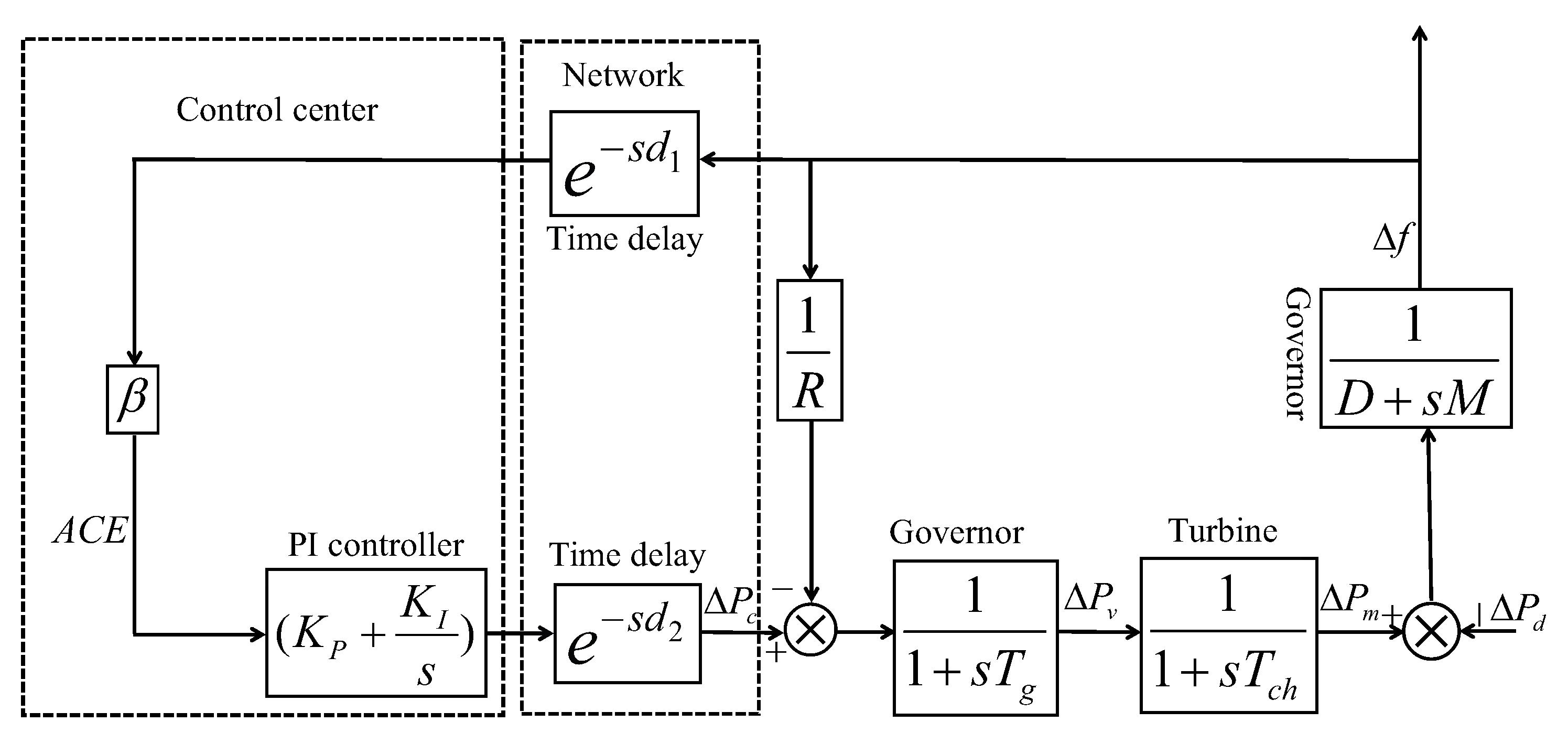
In this subsection, the model of one-area power system equipped with PI controllers and taking into account the time-varying communication delays is given. The basic diagram of the simplified LFC of one-area power system is shown in Figure 1, where and are time delays, respectively, arising during the measured signal transmitted from sensor to the LCF center and the control signal sent from the control center to the governor.
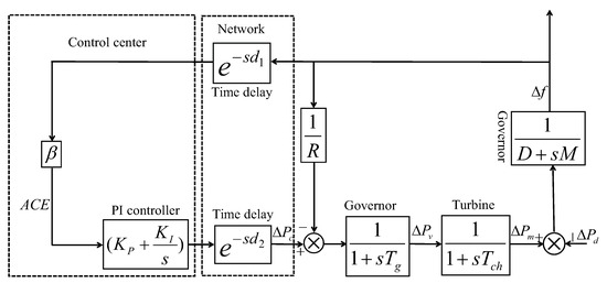
Figure 1.
The basic diagram of the simplified LFC of one-area power system.
According to the LFC system shown in [19] and Figure 1, the common LFC scheme model of one-area can be expressed as follows:
where
Here, , and are the frequency deviation, the mechanical output change, and the valve position change, respectively; M and D are the moment of inertia of the generator and generator damping coefficient, respectively; and are the time constant of the governor and the turbine, respectively; R is the speed droop; is the setpoint; and is the frequency bias factor. The following PI controller is used as the LFC scheme:
where and are PI gains; and the is the area control error. Due to the existence of time-varying delays ( and ) in feedback and forward channels, respectively, the following is obtained
By defining virtual state and measurement output vector as and , the closed-loop LFC system can be expressed as the following linear system with two additive time-varying delays:
and the system parameters are listed in the following form
2.2. Two-Area LFC System
In this subsection, models of two-area power system equipped with PI controllers and taking into account the time-varying communication delays are given. The basic diagram of the simplified LFC of two-area power system is shown in Figure 2, where and are the tie-line power transfer and synchronising coefficient of the tie-line. According to the LFC system shown in [20] and Figure 2, the ACE can be expressed as follows:
and the closed-loop LFC system with PI controllers and time-varying communication delays can be described as follows:
where
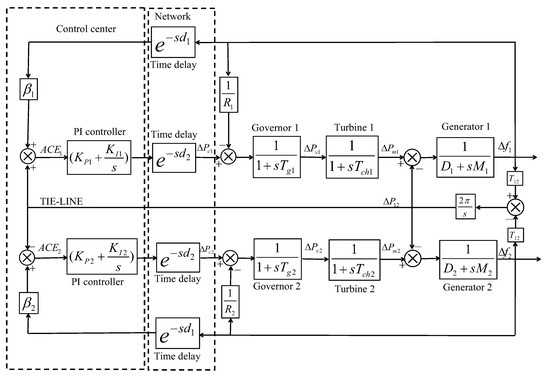
Figure 2.
The basic diagram of the simplified LFC of two-area power system.
As discussed in the Introduction section, the communication channel may encounter time delays, which are usually time-varying and bounded. Then, similar to the previous work, the delays are expressed by time-varying functions satisfying the following conditions:
where , , and are positive constants. Let and .
3. Stability Assessment for LFC System
Lemma 1
([33]). For a positive definite matrix R and differentiable function x in , the following holds
where , with , , .
Lemma 2
([30]). For positive definite matrices , , vectors , and a scalar , if there exists symmetric matrices and any matrices such that
the following inequality holds
Lemma 3
([39]). Let symmetric matrices , , and a vector . Then, the following inequality
holds for all if and only if there exists a positive definite matrix and a skew-symmetric matrix such that
where and .
Theorem 1.
with , , ,
where the notations of other symbols and matrices can be found in Appendix A and Appendix B.
Proof.
Refer to Appendix C. □
Remark 1.
The stability sufficient condition of the LFC system (4) is obtained in Theorem 1, which can guarantee the stability of the LFC system (4) in the range of the maximum allowable time delay. Compared with the literature [11,17,18,21], the Theorem 1 in this paper further reduces the conservativeness via the augmented LKF application. The main improvements of the LKF are summarized as: (a) introducing four delay-dependent non-integral terms to the LKF, such as , (); (b) introducing some integral components to the single-integral terms under different time-varying delay subintervals, such as , , , , and so on. These improvements make the LKF contain more information of the time-varying delay and the coupling information between the state variables and the delay than the literature [11,17,18,21], which reduces the conservativeness caused by the LKF construction.
Remark 2.
It is well known that in order to improve the conservativeness of the stability criterion, the modified LKF must combine with some tight inequality technique [36]. Therefore, Lemmas 1 and 2 are used to estimate the derivative of the LKF, where some effective auxiliary functions and free-weight matrices are introduced into the upper bound on the derivative of the LKF. Finally, Theorem 1 based on the modified LKF and two proper inequality techniques is less conservative than those of the recently published literature [11,17,18,21].
Remark 3.
However, according to the inequality (A8) in the proof process, the final form of the upper bound on the derivative of the LKF is nonlinear due to , which cannot be solved by MATLAB. The authors of [25] decomposed this nonlinear matrix inequality into three equivalent LMI conditions via the sufficient condition constraint lemma application. It reduced the degree of freedom for solving the matrix inequality in the main theorem, due to the introduction of two additional LMI constraints. Moreover, the sufficient condition constraint lemma is quite conservative [39]. To overcome the nonlinear matrix inequality in the stability criterion, the novel negative definite inequality equivalent transformation lemma (Lemma 3) proposed in [39] is used to transform the inequality (A8) to the LMI (12) equivalently, which can be easily solved by the MATLAB LMI-Toolbox.
4. Results and Discussions
In this section, the effectiveness of the stability criterion proposed in this paper is shown. For different and values, the maximum allowable time-delay upper bound values (MADUB) can be obtained by solving the LMIs in Theorem 1 via Matlab LMI-Toolbox. The LFC system parameters in Table 1 are given in [20]. One and two-area LFC systems will be discussed and comparatively analyzed in the following subsections. In the following subsections, ‘–’ in the tables indicates that the corresponding result is not given.

Table 1.
LFC systems parameters with pu/rad.
4.1. One-Area LFC System
4.1.1. Conservativeness Comparisons
In order to compare with the existing results, Table 2 and Table 3 give the MADUB values of the case of fixed and values, , , , . The corresponding results cannot be given in [11,17,18] since the time delays from sensor to the LFC center are ignored. Moreover, to show the PI controller gains influence on the MADUB of the LFC system, Table 4 obtains the MADUB values of the case of different , values, and ; Table 5 gives the MADUB values of the case of different , values, and . From these tables, it can observe the results of Theorem 1 are similar to those of [11], however, less conservative than those of [14,15,16,19,20,21]. Meanwhile, the MADUB increases with increment at a fixed value, and the MADUB decreases with increment at a fixed value.
Table 2.
MAUBs for given , and under one-area LFC system.
Table 3.
MAUBs for given , and under one-area LFC system.
Table 4.
MAUBs for and under one-area LFC system.
Table 5.
MAUBs for and under one-area LFC system.
4.1.2. Simulation Verification
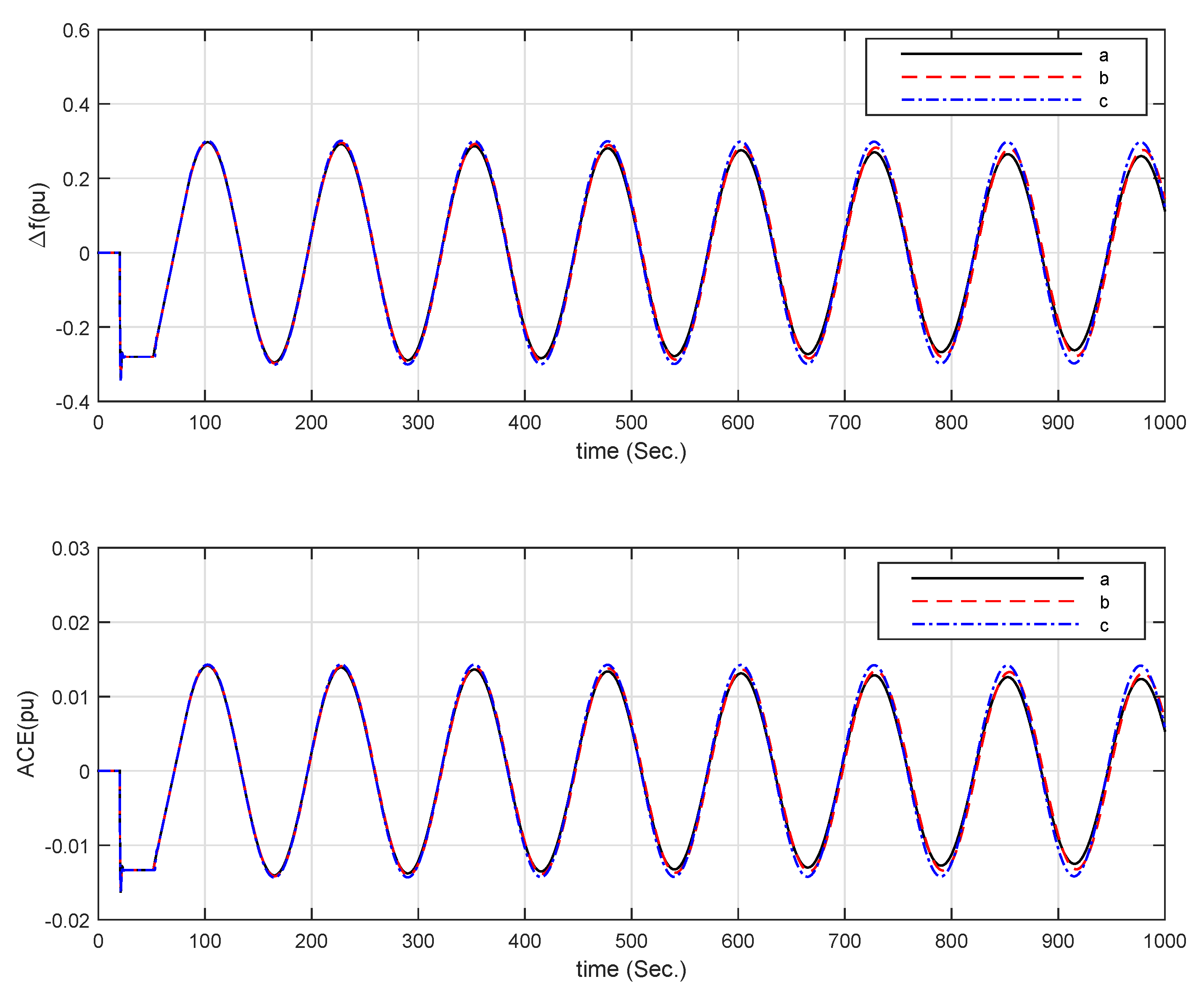
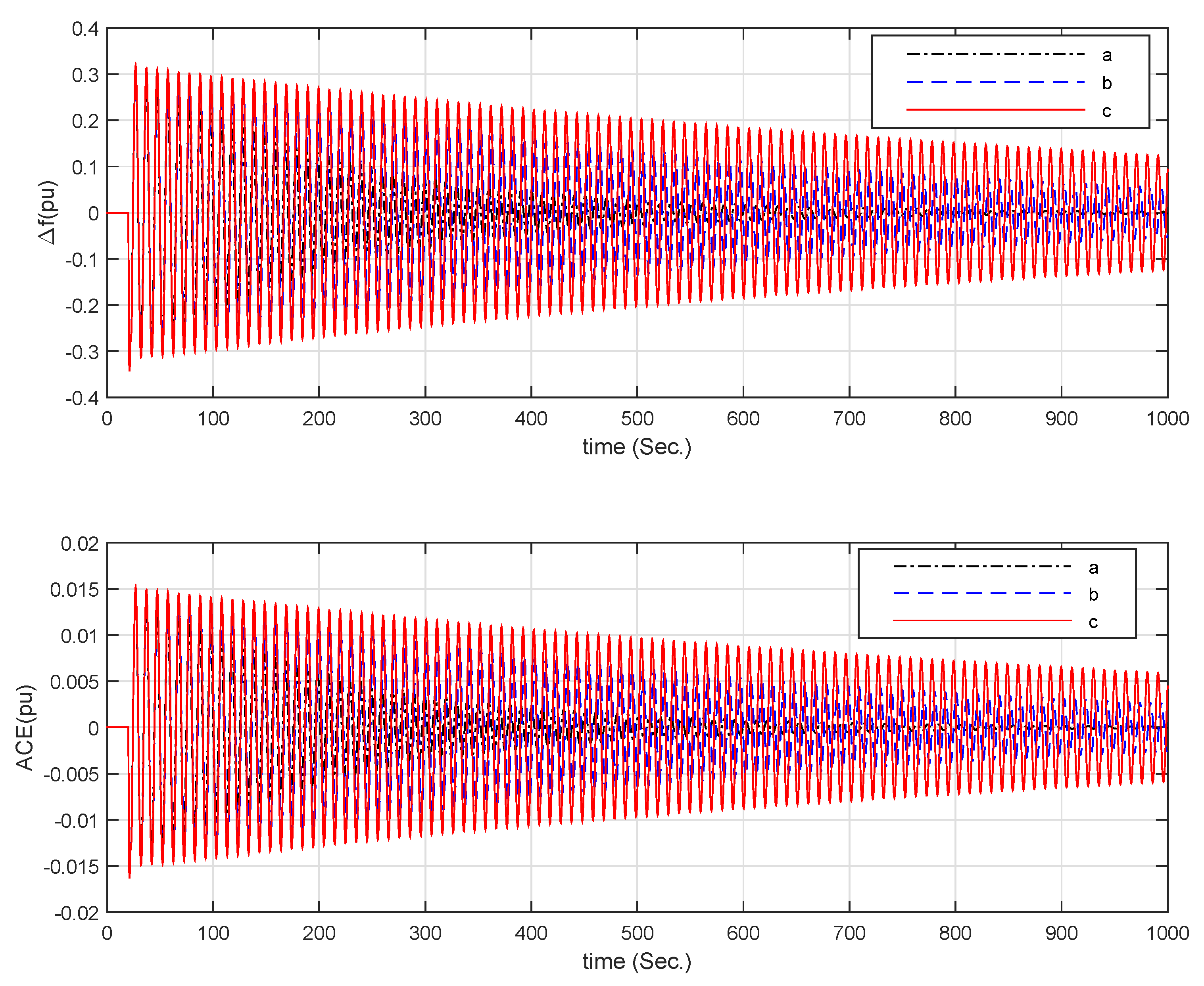
Simulation studies are carried out under an increased step load of 0.1 pu occurring at 1 s, time-varying delays and the following assumptions. The simulation results are shown in Figure 3, Figure 4, Figure 5 and Figure 6, in which the LFC has achieved its objective, and the control system is stable. In Figure 4, the blue curve is close to the critical stability with , , and .
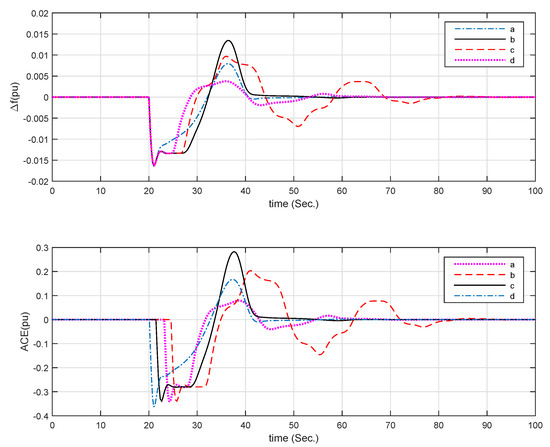
Figure 3.
Frequency deviation and control error responses of one-area deregulated LFC scheme with , and different time-varying delays.
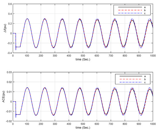
Figure 4.
Frequency deviation and control error responses of one-area deregulated LFC scheme with , and different , .
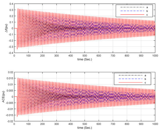
Figure 5.
Frequency deviation and control error responses of one-area deregulated LFC scheme with , and different , .
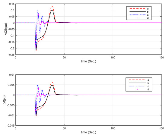
Figure 6.
Frequency deviation and control error responses of one-area deregulated LFC scheme with and different , and time-varying .
4.2. Two-Area LFC System
4.2.1. Conservativeness Comparison
Table 6 and Table 7 give the MADUB values of the case of fixed and values, , and different , values. The corresponding results cannot be achieved in [11,17,18] since the time delays from sensor to the load frequency control center are ignored. Table 8 gives the MADUB values of the case of different and values, and ; and Table 9 give the MADUB values of the case of different and values, and . From these tables, it is obviously that the MADUB increases with increment at a fixed value, and the MADUB decreases with increment at a fixed value. In addition, the results of Theorem 1 are less conservative than those of [11,15,20].
Table 6.
MAUBs for given , and under two-area LFC system.
Table 7.
MAUBs for given , and under two-area LFC system.
Table 8.
MAUBs for and under two-area LFC system.
Table 9.
MAUBs for and under two-area LFC system.
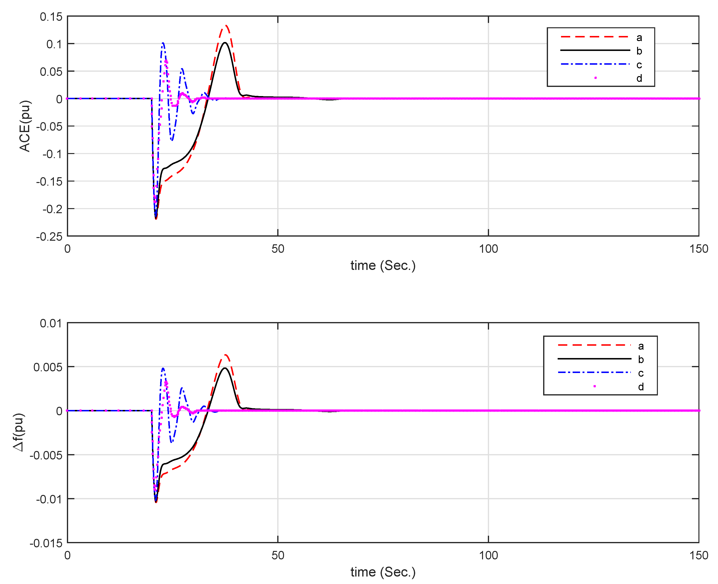
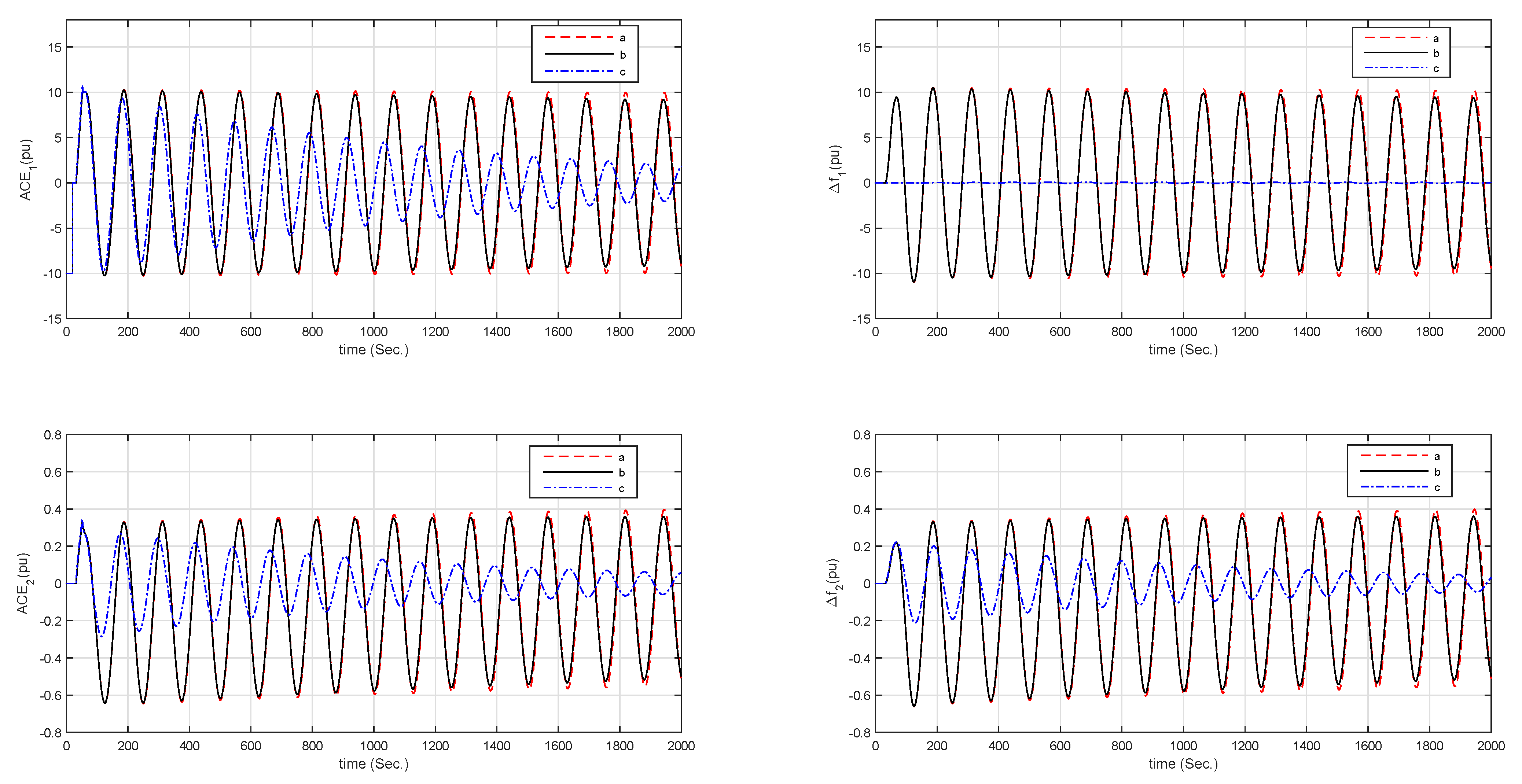
4.2.2. Simulation Verification
Simulation studies are carried out under an increased step load of 0.1 pu occurring at 1 s, and time-varying delays and the following assumptions:
- For Figure 7, fixed , :
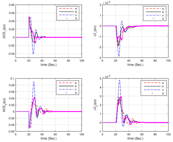 Figure 7. Frequency deviation and control error responses of two-area deregulated LFC scheme with , and time-varying delays.
- , ;
- , ;
- , ;
- , ;
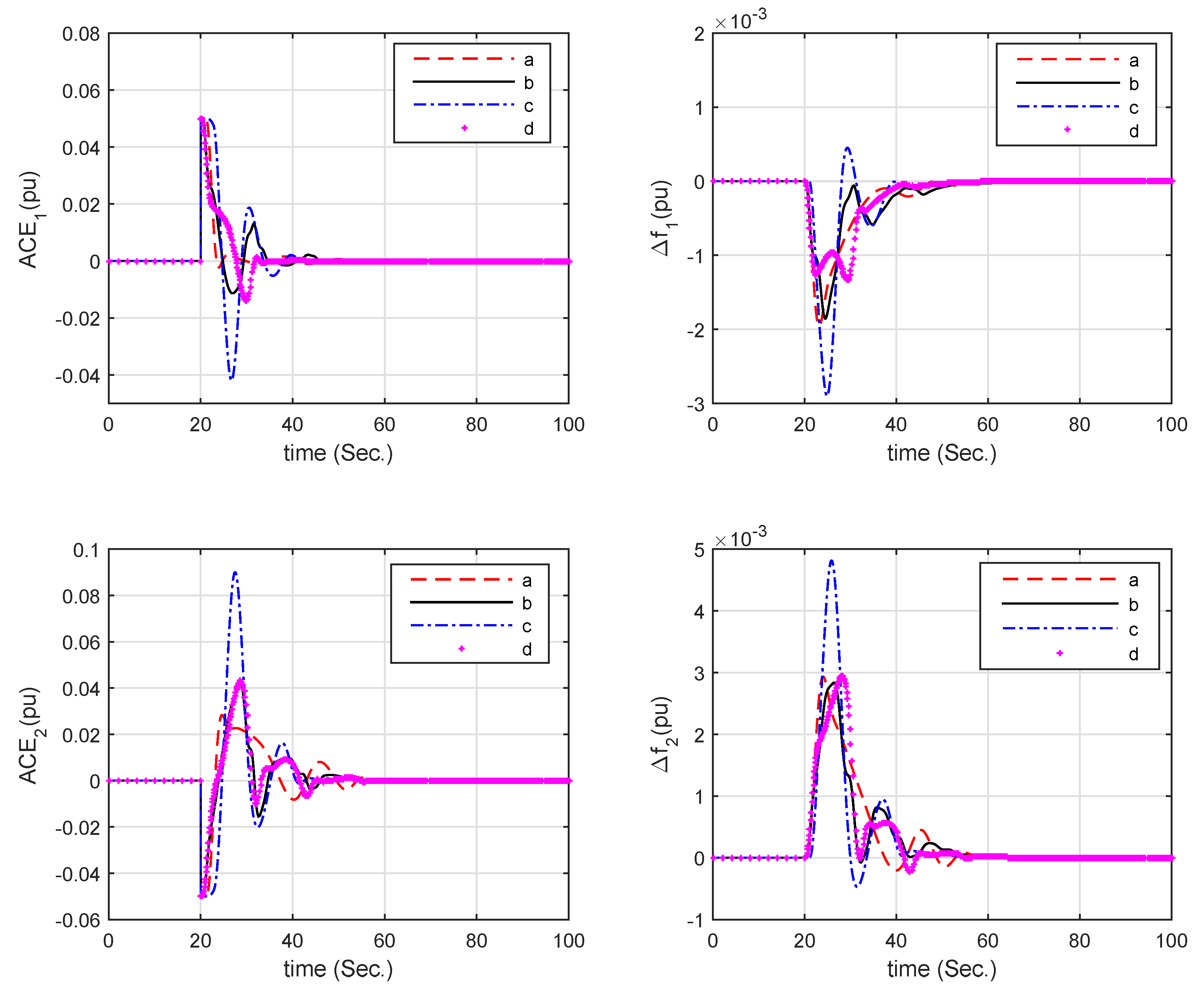
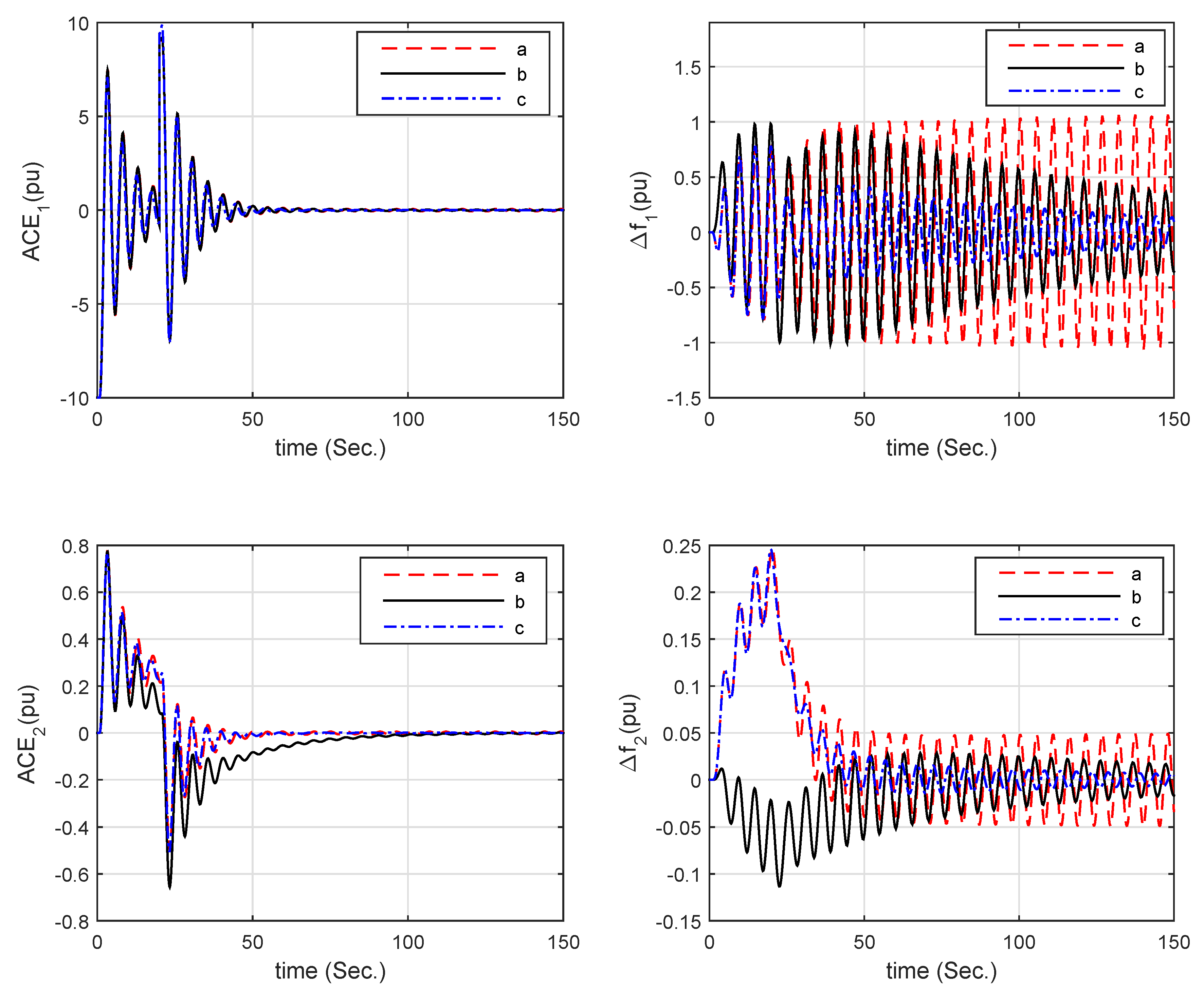
- For Figure 8, different and fixed , :
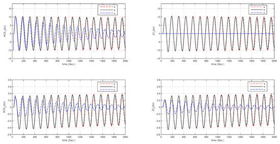 Figure 8. Frequency deviation and control error responses of two-area deregulated LFC scheme with , and different , .
- , ;
- , ;
- , ;
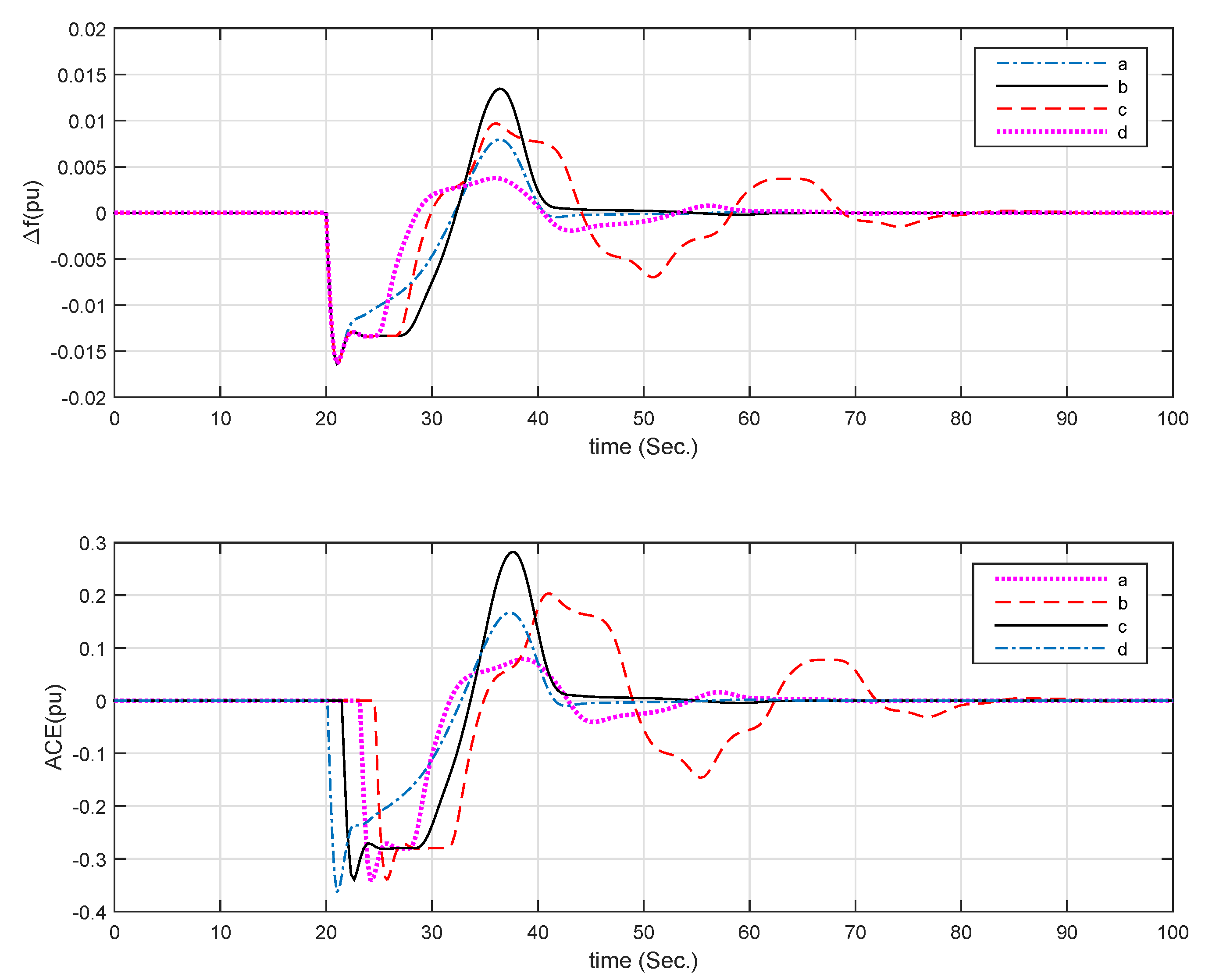
- For Figure 9, different and fixed , :
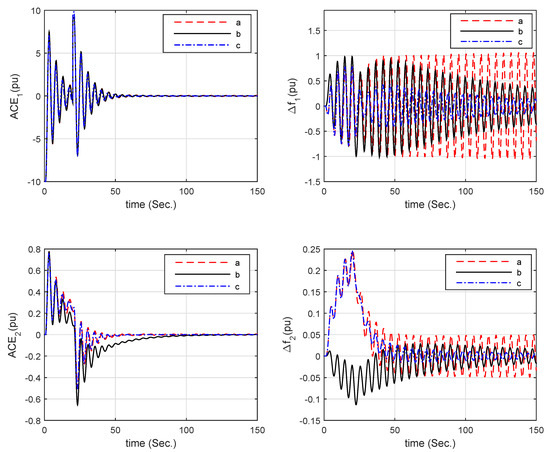 Figure 9. Frequency deviation and control error responses of two-area deregulated LFC scheme with , and different , .
- , ;
- , ;
- , ;
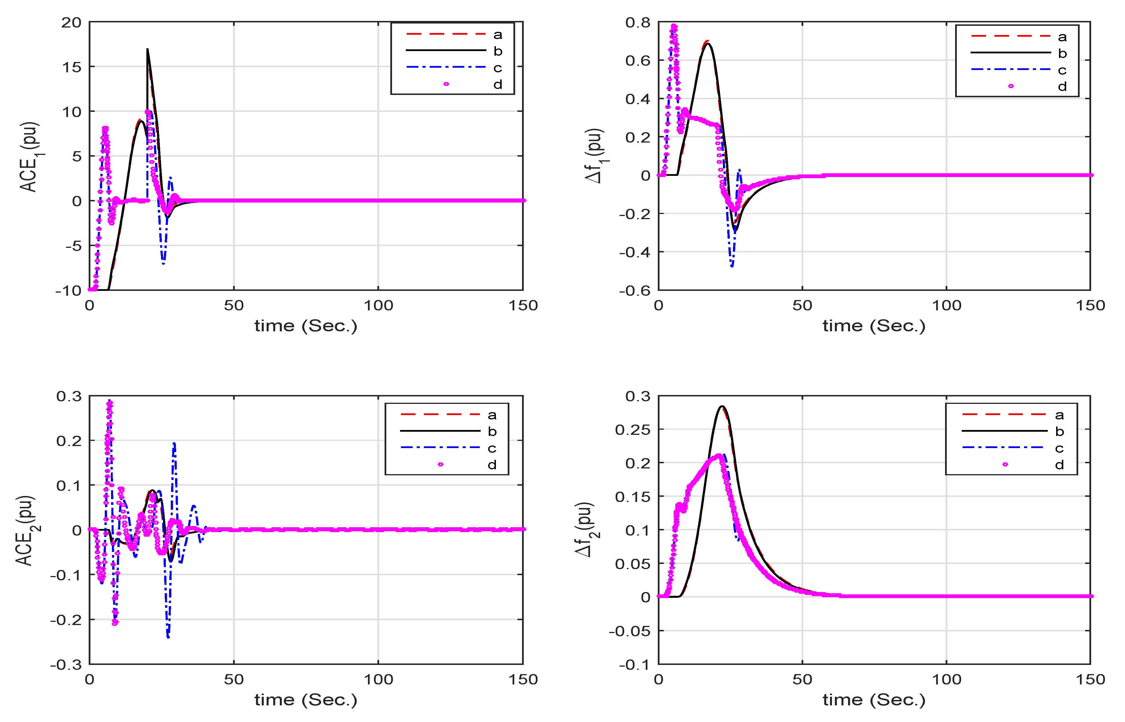
- For Figure 10, different , , time-varying and fixed :
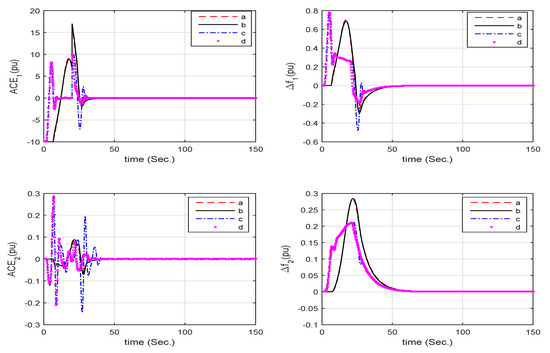 Figure 10. Frequency deviation and control error responses of two-area deregulated LFC scheme with and different , , .
- , , ;
- , , ;
- , , ;
- , , .
The simulation results are shown in Figure 7, Figure 8, Figure 9 and Figure 10, in which the LFC has achieve its objective, and the control system is stable. It can be seen from Figure 8 and Figure 9 that the red curves are the critical stability with , , , and , , , , respectively. Thus, the black curvess in Figure 8 and Figure 9 are close to the critical stability region, that is, Theorem 1 proposed in this paper is effective in estimating the upper bound of the maximum allowable time delay.
5. Conclusions
This paper mainly focuses on the stability analysis for load frequency control of power systems with time-varying delays. For the one-area and two-area LFC systems with two communication delays, stability criteria are obtained via Lyapunov stability theory application. Firstly, the one-area LFC system and two-area LFC system are described as linear systems with additive time-varying delays. Secondly, a modified LKF with some delay-dependent non-integral terms and augmented integral components in single integral term is constructed. Compared with the LKFs in some previous published literature, it contains more coupling information between time-varying delays and state variables, which reduces the conservativeness of the stability criterion. Thirdly, to overcome the nonlinear coupling in the stability criterion, the novel negative definite inequality equivalent transformation lemma (Lemma 3) is used to transform the nonlinear inequality to the LMI equivalently, which can be easily solved by the MATLAB LMI-Toolbox. Finally, the effectiveness of the proposed method is illustrated by comparisons and discussions in numerical examples. In addition, in order to approach the actual situation, the design and optimization of the controllers have always been a topic of concern, which inspires us to work around it in the future. The stability results can be applied to the LFC design and optimization to guarantee the stable operation of power system based on an open interconnect network control.
However, there are some limitations. Firstly, in order to reduce the conservativeness of the stability criterion, the dimensions of the decision variables for solving LMIs increase with the expanded dimensions of LKF. Secondly, in order to improve the degree of freedom of solving LMIs, the free weight matrices are introduced. Thirdly, some additional decision variables are introduced in LMIs when the nonlinear inequalities are transformed into LMIs by using Lemma 3, which increases the number of decision variables of the LMIs proposed in this paper. In conclusion, the improvement of stability results is in the cost of increasing computational complexity.
The derivation method of the stability criterion presented in this paper can be extended to multi-area LFC system. The relevant theories will be applied into practice, which is one of our further main topics.
Author Contributions
Conceptualization, W.F. and Y.X.; data curation, F.L.; methodology, W.F. and W.D.; software, X.Z.; writing—original draft, W.F.; writing—review and editing, F.L. and X.Z. All authors have read and agreed to the published version of the manuscript.
Funding
This work is supported partly by the Natural Science Foundation of Guangdong Province under Grant 2018A0303130111, the Industry University Research Cooperation Project of Jiangsu Province under Grant BY2020649 and the Yellow Sea Rookie of Yancheng Institute of Technology.
Institutional Review Board Statement
Not applicable.
Informed Consent Statement
Not applicable.
Data Availability Statement
Not applicable.
Conflicts of Interest
The authors declare no conflict of interest.
Appendix A
For the sake of simplicity on matrix representation, the notations of several symbols and matrices are defined as
Appendix B
Notations of other symbols and matrices for the Theorem 1 are given as:
Appendix C
Proof of Theorem 1.
Construct an LKF candidate as
with
where , , and .
Calculating the derivative of , we can obtain the following formulas
According to , (), letting and , it follows from Lemmas 1 and 2 that
For an appropriately matrix , we can get
According to Lemma 3, the matrix inequality (11) together with the matrix inequality (12) imply that . Therefore, by Lyapunov stability theorem, it can guarantee that the time-delayed system (4) is asymptotically stable. The proof is completed. □
References
- Kundur, P. Power System Stability and Control; McGraw-Hill: New York, NY, USA, 1994. [Google Scholar]
- Mello, R.; Apostolopoulou, D.; Alonso, E. Cost efficient distributed load frequency control in power systems. In Proceedings of the 21st IFAC World Congress, Berlin, Germany, 12–17 July 2020; Volume 53, pp. 8037–8042. [Google Scholar]
- Ali, D.; Mohammad, M.; Zeinolabedin, M.; Lieven, V. A novel technique for load frequency control of multi-area power systems. Energies 2020, 13, 2125. [Google Scholar]
- Giudice, D.; Brambilla, A.; Grillo, S.; Bizzarri, F. Effects of inertia, load damping and dead-bands on frequency histograms and frequency control of power systems. Int. J. Electr. Power Energy Syst. 2021, 129, 106842. [Google Scholar] [CrossRef]
- Ladygin, A.; Bogachenko, D.; Kholin, V. Efficient control of induction motor current in a frequency—Ccontrolled electric drive. Russ. Electr. Eng. 2020, 6, 362–367. [Google Scholar] [CrossRef]
- Baykov, D.; Gulyaev, I.; Inshakov, A.; Teplukhov, D. Simulation modeling of an induction motor drive controlled by an array frequency converter. Russ. Electr. Eng. 2019, 7, 485–490. [Google Scholar] [CrossRef]
- Aminov, R.; Garievskii, M. Effect of engagement in power and frequency control on the service life of steam–turbine power units. Power Technol. Eng. 2019, 53, 479–483. [Google Scholar] [CrossRef]
- Khalil, A.; Peng, A. An accurate method for delay margin computation for power system stability. Energies 2018, 11, 3466. [Google Scholar] [CrossRef] [Green Version]
- Jin, L.; Zhang, C.; He, Y.; Jiang, L.; Wu, M. Delay-dependent stability analysis of multi-area load frequency control with enhanced accuracy and computation efficiency. IEEE Trans. Power Syst. 2019, 34, 3687–3696. [Google Scholar] [CrossRef]
- Martin, G.; Begovic, M.; Taylor, D. Transient control of generator excitation in consideration of measurement and control delays. IEEE Trans. Power Deliv. 2002, 10, 135–141. [Google Scholar] [CrossRef]
- Manikandan, S.; Kokil, P. Stability analysis of load frequency control system with constant communication delays. IFAC PapersOnLine 2020, 53, 338–343. [Google Scholar] [CrossRef]
- Zhang, C.; Jiang, L.; Wu, Q.; He, Y.; Wu, M. Further results on delay-dependent stability of multi-area load frequency control. IEEE Trans. Power Syst. 2015, 28, 4465–4474. [Google Scholar] [CrossRef]
- Peng, C.; Zhang, J. Delay-distribution-dependent load frequency control of power systems with probabilistic interval delays. IEEE Trans. Power Syst. 2016, 31, 3309–3317. [Google Scholar] [CrossRef]
- Ramakrishnan, K.; Ray, G. Stability criteria for nonlinearly perturbed load frequency systems with time-delay. Electr. Power Compon. Syst. 2017, 45, 302–314. [Google Scholar] [CrossRef]
- Sönmez, A.; Nwankpa, C. An exact method for computing delay margin for stability of load frequency control systems with constant communication delays. IEEE Trans. Power Syst. 2016, 31, 370–377. [Google Scholar] [CrossRef]
- Yang, F.; He, J.; Wang, D. New stability criteria of delayed load frequency control systems via infinite-series-based inequality. IEEE Trans. Ind. Inform. 2018, 14, 231–240. [Google Scholar] [CrossRef]
- Chen, B.; Shangguan, X.; Jin, L.; Li, D. An improved stability criterion for load frequency control of power systems with time-varying delays. Energies 2020, 13, 2101. [Google Scholar] [CrossRef] [Green Version]
- Shen, H.; Jiao, S.; Park, J.; Sreeram, V. An improved result on H∞ load frequency control for power systems with time delays. IEEE Syst. J. 2020, 15, 3238–3248. [Google Scholar] [CrossRef]
- Xu, H.; Zhang, C.; Jiang, L.; Smitha, J. Stability analysis of linear systems with two additive time-varying delays via delay-product-type Lyapunov functional. Appl. Math. Model. 2017, 45, 955–964. [Google Scholar] [CrossRef]
- Jiang, L.; Yao, W.; Wu, Q.; Wen, J.; Chen, S. Delay-dependent stability for load frequency control with constant and time-varying delays. IEEE Trans. Power Syst. 2012, 27, 932–941. [Google Scholar] [CrossRef]
- Shen, C.; Li, Y.; Zhu, X.; Duan, W. Improved stability criteria for linear systems with two additive time-varying delays via a novel Lyapunov functional. J. Comput. Appl. Math. 2019, 363, 312–324. [Google Scholar] [CrossRef]
- Hua, C.; Qiu, Y.; Wang, Y.; Guan, X. An augmented delays-dependent region partitioning approach for recurrent neural networks with multiple time-varying delays. Neurocomputing 2021, 423, 248–254. [Google Scholar] [CrossRef]
- Duan, W.; Li, Y.; Chen, J. Further stability analysis for time-delayed neural networks based on an augmented Lyapunov functional. IEEE Access 2019, 7, 104655–104666. [Google Scholar] [CrossRef]
- Duan, W.; Li, Y.; Chen, J. An enhanced stability criterion for linear time-delayed systems via new Lyapunov-Krasovskii functionals. Adv. Differ. Equ. 2020, 2020, 21. [Google Scholar] [CrossRef]
- Kim, J. Further improvement of Jensen inequality and application to stability of time-delayed systems. Automatica 2016, 64, 121–125. [Google Scholar] [CrossRef]
- Scopus, P.; Tian, Y.; Wang, Z. Stability analysis for delayed neural networks based on the augmented Lyapunov-Krasovskii functional with delay-product-type and multiple integral terms. Neurocomputing 2020, 410, 295–303. [Google Scholar]
- Gholami, Y. Existence and global asymptotic stability criteria for nonlinear neutral-type neural networks involving multiple time delays using a quadratic-integral Lyapunov functional. Adv. Differ. Equ. 2021, 112, 2021. [Google Scholar]
- Duan, W.; Fu, X.; Yang, X. Further results on the robust stability for neutral-type Lur’e system with mixed delays and sector-bounded nonlinearities. Int. J. Control Autom. Syst. 2016, 14, 560–568. [Google Scholar] [CrossRef]
- Duan, W.; Fu, X.; Liu, Z. Improved robust stability criteria for time-delay Lur’e system. Int. J. Control Autom. Syst. 2017, 19, 139–150. [Google Scholar] [CrossRef]
- Zhang, X.; Han, Q.; Seuret, A.; Gouaisbaut, F. An improved reciprocally convex inequality and an augmented Lyapunov-Krasovskii functional for stability of linear systems with time-varying delay. Automatica 2017, 84, 221–226. [Google Scholar] [CrossRef] [Green Version]
- Duan, W.; Li, Y.; Sun, Y.; Chen, J.; Yang, Y. Enhanced master-slave synchronization criteria for chaotic Lur’e systems based on time-delayed feedback control. Math. Comput. Simul. 2020, 177, 276–294. [Google Scholar] [CrossRef]
- Gu, K. An integral inequality in the stability problem of time-delay systems. In Proceedings of the Conference of the IEEE Industrial Electronics, Sydney, Australia, 12–15 December 2010. [Google Scholar]
- Seuret, A.; Gouaisbaut, F. Hierarchy of LMI conditions for the stability analysis of time-delay systems. Syst. Control Lett. 2015, 81, 1–7. [Google Scholar] [CrossRef] [Green Version]
- Feng, W.; Luo, F.; Duan, W.; Chen, J. An improved stability criterion for linear time-varying delay systems. Automatika 2020, 61, 229–237. [Google Scholar] [CrossRef]
- Kwon, N.; Lee, S. An affine integral inequality of an arbitrary degree for stability analysis of linear systems with time-varying delays. IEEE Access 2021, 9, 51958–51969. [Google Scholar] [CrossRef]
- Zhang, C.; He, Y.; Jiang, L.; Wu, M. Notes on stability of time-delay systems: Bounding inequalities and augmented Lyapunov-Krasovskii functionals. IEEE Trans. Autom. Control 2017, 62, 5331–5336. [Google Scholar] [CrossRef] [Green Version]
- Duan, W.; Du, B.; Li, Y.; Shen, C.; Zhu, X.; Li, X.; Chen, J. Improved sufficient LMI conditions for the robust stability of time-delayed neutral-type Lur’e systems. Int. J. Control Autom. Syst. 2018, 16, 2343–2353. [Google Scholar] [CrossRef]
- Duan, W.; Li, Y.; Chen, J. New results on stability analysis of uncertain neutral-type Lur’e systems derived from a modified Lyapunov-Krasovskii functional. Complexity 2019, 2019, 1706264. [Google Scholar] [CrossRef]
- de Oliveira, F.S.; Souza, F.O. Further refinements in stability conditions for time-varying delay systems. Appl. Math. Comput. 2020, 369, 124866. [Google Scholar] [CrossRef]

Publisher’s Note: MDPI stays neutral with regard to jurisdictional claims in published maps and institutional affiliations. |
© 2021 by the authors. Licensee MDPI, Basel, Switzerland. This article is an open access article distributed under the terms and conditions of the Creative Commons Attribution (CC BY) license (https://creativecommons.org/licenses/by/4.0/).