Article

Exploring the Exhaust Emission and Efficiency of Algal Biodiesel Powered Compression Ignition Engine: Application of Box–Behnken and Desirability Based Multi-Objective Response Surface Methodology

1
School of Engineering Sciences, Delhi Skill and Entrepreneurship University, Delhi 110089, India
2
Sustainable and Renewable Energy Engineering Department, University of Sharjah, Sharjah P.O. Box 27272, United Arab Emirates
3
U.S.-Pakistan Center for Advanced Studies in Energy (USPCAS-E), National University of Sciences and Technology (NUST), Islamabad 44000, Pakistan
4
Advanced Renewable and Sustainable Energy Research Group, Scientific Research Center, Al-Ayen University, Thi-Qar 64001, Iraq
5
Solar Thermal Vacuum Engineering Research Group, London Centre for Energy Engineering, School of Engineering, London South Bank University, London SE1 0AA, UK
*
Authors to whom correspondence should be addressed.
Energies 2021, 14(18), 5968; https://doi.org/10.3390/en14185968
Submission received: 11 September 2021 / Revised: 17 September 2021 / Accepted: 17 September 2021 / Published: 20 September 2021
(This article belongs to the Special Issue Applied Solar Thermal Energy)

Abstract

:
Sustainable Development Goals were established by the United Nations General Assembly to ensure that everyone has access to clean, affordable, and sustainable energy. Third-generation biodiesel derived from algae sources can be a feasible option in tackling climate change caused by fossil fuels as it has no impact on the human food supply chain. In this paper, the combustion and emission characteristics of Azolla Pinnata oil biodiesel-diesel blends are investigated. The multi-objective response surface methodology (MORSM) with Box–Behnken design is employed to decrease the number of trials to conserve finite resources in terms of human labor, time, and cost. MORSM was used in this study to investigate the interaction, model prediction, and optimization of the operating parameters of algae biodiesel-powered diesel engines to obtain the best performance with the least emission. For engine output prediction, a prognostic model is developed. Engine operating parameters are optimized using the desirability technique, with the best efficiency and lowest emission as the criteria. The results show Theil’s uncertainty for the model’s predictive capability (Theil’s U2) to be between 0.0449 and 0.1804. The Nash–Sutcliffe efficiency is validated to be excellent between 0.965 and 0.9988, whilst the mean absolute percentage deviation is less than 4.4%. The optimized engine operating conditions achieved are 81.2% of engine load, 17.5 of compression ratio, and 10% of biodiesel blending ratio. The proposed MORSM-based technique’s dependability and robustness validate the experimental methods.

1. Introduction

The United Nations General Assembly (UNGA) created the Sustainable Development Goals (SDGs) in 2015. They are a collection of 17 linked global objectives. By 2030, the SDGs are supposed to create an “outline for a better and more sustainable future for everybody.” The Sustainable Development Goals (SDGs) were created to replace the Millennium Development Goals, which were in force until 2015 [1]. One such SDG is Sustainable Development Goal 7 (SDG 7 or Global Goal 7). The organization’s mission is to “ensure that everyone has access to affordable, reliable, contemporary, and sustainable energy.” People’s well-being, as well as economic progress and poverty alleviation, are all dependent on access to energy. Five goals must be fulfilled by 2030 to achieve the net-zero emissions target [2]. Diesel engines are widely utilized in off-grid energy production, agriculture, industrial, land transportation, and maritime transportation. It is recommended due to its reliability, low initial cost, simple maintenance, and higher energy conversion efficiency [3]. Their exhaust, on the other hand, comprises hazardous greenhouse gases (GHGs). GHGs are the primary cause of climate change, resulting in global warming, erratic weather patterns, soil fertility loss, and the submergence of low-lying islands. GHGs also contribute to air pollution, which has negative health consequences. The majority of emerging countries, such as India, are heavily reliant on fossil fuel imports. Indeed, fossil fuel consumes a significant percentage of the country’s gross domestic product. With the use of alternative energy sources, this dual-faced problem of GHGs and imports may be significantly minimized. Biodiesel, producing gas, and natural gas are examples of alternative fuels that may be utilized in a diesel engine [4].
Biofuel research has received significant attention over the last few decades, and researchers have been investigating a variety of feedstocks. Biofuels are generally classified into three generations. First-generation biofuels include edible oils, bio-alcohols, biogas, biodiesel, solid biofuels, etc. These 1st generation biofuels make use of simple techniques to convert sugar, edible oil, and animal fats into fuel. These 1st generation biofuels have caused disagreement among environmentalists. If biofuels are preferred over food supplies, the food problem will worsen. Secondly, these 1st generation biofuels also have the limitations of net total energy loss, e.g., ethanol production requires more energy than it produces, hence resulting in a total energy loss. These 1st generation biofuels also promote deforestation and create a scarcity of water in some regions [5]. According to the WHO, bio-crops should be best used for meeting food supply rather than as a fuel source. These problems with 1st generation biofuel motivate researchers to focus on other alternatives to biofuel. This led to the development of next-generation biofuels that fall under 2nd generation biofuel and are generally produced from nonedible crops. The 2nd generation biofuel includes vegetable oils, bio-hydrogen, bio-alcohols, bio-methanol, and/or biogas sourced from the non-edible feedstock. These second-generation biofuels, however, have certain drawbacks. These biofuels require specific processing to convert feedstock to ethanol, have a poor yield, and can increase deforestation and water scarcity, much as feedstock cannot be used to make biodiesel [3,6].
Researchers are working hard to develop better, more sustainable, and efficient ways to reduce the fuel problem due to the limits of 2nd generation biofuels. As a result of these tireless efforts by scientists and researchers, 3rd generation biofuel has been developed. Algae-derived biofuels are included in this third-generation biofuel [7,8]. The use of algae as a fuel was first proposed by German scientists Harder et al. in 1942, and following WWII, different countries across the world began to investigate this subject. Algae microorganisms have two key characteristics, according to researchers. For starters, algae may create an oil that can be utilized to make a variety of biodiesel and gasoline. Furthermore, it may be genetically engineered to directly generate anything from ethanol and butanol to gasoline and diesel fuel [9,10]. In 2021, Jacob et al. [11] presented findings on biodiesel synthesis from microalgae, highlighting its viability and shedding some light on future bioenergy, particularly for I.C. engine applications. Because of their tiny form, third-generation microalgae feedstock culture and fuel production provide long-term and economic benefits. Each process in the manufacture of microalgae biodiesel, such as growth, harvesting, and extraction, may be improved to eliminate the variables impacting production [12]. Optimized microalgae biodiesel blends may be used to obtain optimum engine maps by calibrating engine parameters during stationary or dynamic engine tests. Several studies have been reported on microalgae-based biodiesel synthesis.
Mubarak et al. [13] utilized Salvinia Molesta sourced algal biodiesel blends to power a diesel engine B20 (20% biodiesel + 80% neat diesel) blend performed best among other blends as the Brake Thermal Efficiency (BTE) was 29.5% and the minimum brake specific fuel consumption (BSFC) was 0.3081 kg/kWh. When compared to diesel, the CO2, CO, unburnt hydrocarbon, NO, and smoke emissions were reduced by 3.38%, 14%, 20.83%, 12.86%, and 10.99%, individually. B20 can therefore be utilized as a diesel engine alternative fuel. Subramaniam et al. [14] used algal biodiesel to power a diesel engine in various proportions (such as 10%, 20%, 30%, 40%, and 100%). The 20% biodiesel blends performed best to improve thermal efficiency and reduce smoke, H.C., CO, and PM emissions. Other emissions, such as nitrogen oxide and carbon dioxide, were found to be marginally higher. Nautiyal et al. [15] used biodiesel made from Spirulina Platensis algae to run a diesel engine. As the amount of biodiesel in the fuel mix is raised, carbon monoxide (C.O.), hydrocarbon (H.C.), and smoke emissions are lowered considerably. At maximum load, H.C. emission decreased from 0.06 g/kWh with diesel to 0.04 g/kWh with B100, while smoke emission decreased from 0.7% with diesel to 0.6% with B100 while NOx emissions increased substantially.
Extensive and repetitive experimental investigations to map the effects of any new/alternative/ different additions on binary or ternary fuel mixes are expensive in terms of fuel cost, man-hours, machine hours. Improved statistical–mathematical approaches and greater computer power can aid in the conservation of these limited resources and the expense of experimental research. Artificial intelligence/data-driven techniques for multi-objective optimization, such as Taguchi L9 orthogonal array (T.A.) [16], particle swarm optimization (PSO), response surface methodology (RSM) [17,18,19,20], Gene expression programming (GEP) [21,22], and artificial neural network (ANN) [22,23], have been successfully implemented for diverse engineering applications. By deducing a mathematical expression between controlled input parameters and their responses, these approaches are utilized to create output prediction models. Once the predictive model is built, it may be used to optimize engine operating parameters for maximum output. To establish a robust predictive-optimized model, the findings may be validated via lab-based tests. Bietresato et al. [24] successfully employed the RSM to optimize the performance of a biodiesel-bioethanol-diesel powered tractor engine. RSM demonstrated strong prediction abilities and produced interesting results. The use of the RSM revealed that the fuel composition has a significant impact on engine performance. The corresponding mathematical models have a good level of fit (R2 > 0.90 for both mechanical and environmental outputs) and prediction abilities.
As such, the third-generation biodiesel is considered a suitable replacement for older generation biodiesels. Even though there are a few publications on the impacts of utilizing microalgae biodiesel in I.C. engines, it requires comprehensive investigations under diverse conditions. It has also been noted that not enough research has been done to enhance the performance and minimize emissions of a diesel engine running on algae biodiesel blends. Furthermore, the use of intelligent optimization techniques like multi-objective response surface methodology (MORSM) to forecast and optimize the operating parameters of an algal biodiesel-powered engine has not been well studied in the literature. As a consequence, MORSM is being used in this study to investigate the interaction, model prediction, and optimization of the operating parameters of algae biodiesel-powered diesel engines to obtain the best performance and emission characteristics.

2. Materials and Methods

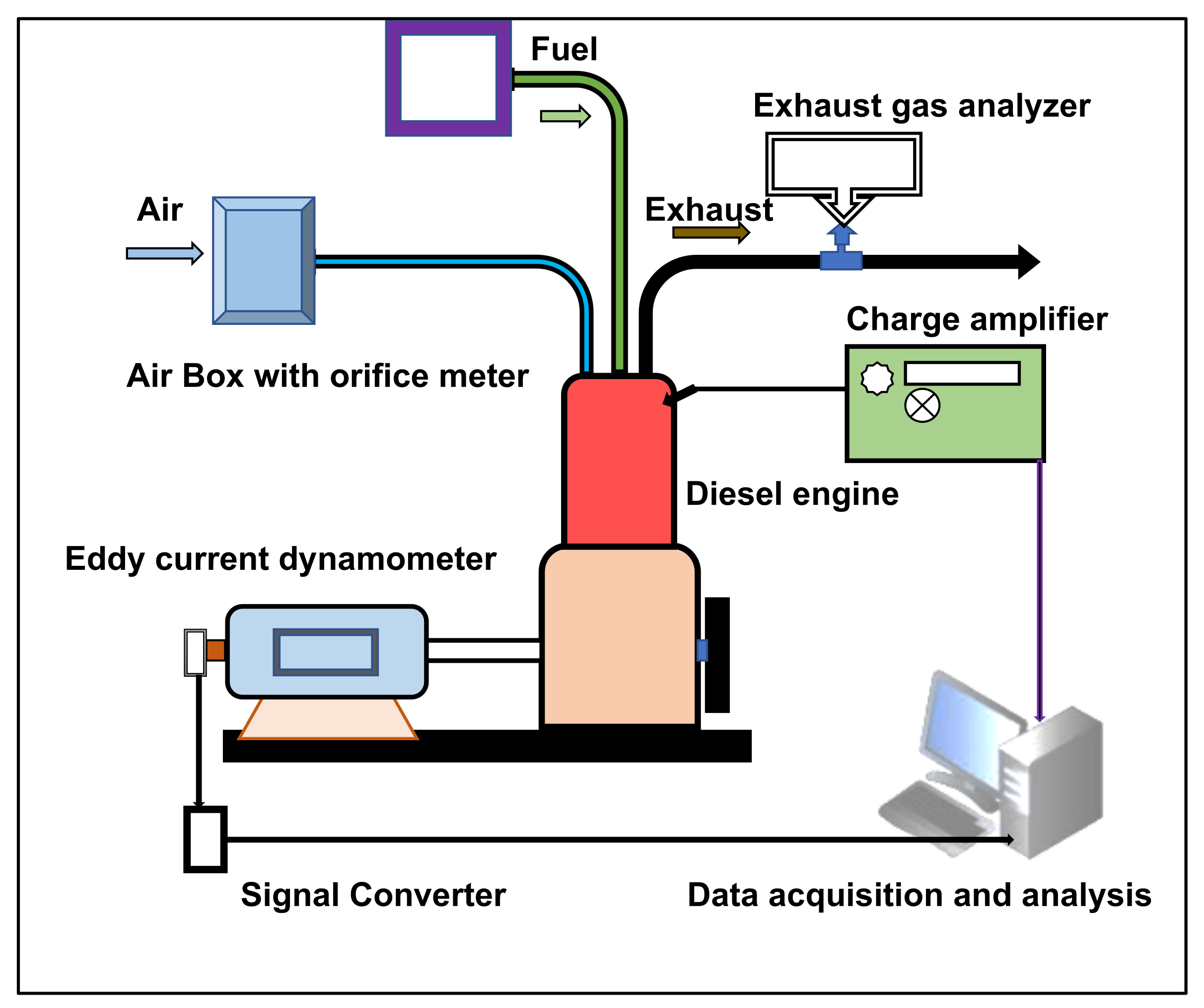
2.1. Setup for the Test

The current study employed a contemporary computerized engine test setup with a small variable compression CI engine (single-cylinder four-stroke), similar to those extensively used in diesel generator sets or irrigation pumps. The test engine was a water-cooled type provision of varying compression ratio. The test bench had the provision for engine loading unit (eddy current type), cooling water, and fuel supply measuring units. The engine load can be varied by the knob provided on the control panel, as it controls the electric current to a dynamometer. The cooling water flow rate to the engine as well as dynamometer was measured with two rotameters installed on the test bench. A piezoelectric type pressure sensor was used to monitor the pressure within the engine cylinder, and a thermocouple unit was used to detect the exhaust gas temperature near the engine exhaust outlet. A five-gas exhaust testing unit was used for emission measurement. The test engine setup’s complete characteristics are provided in Table 1. An orifice meter in an airbox was used to measure airflow, while a glass burette on the test bench was used to monitor fuel flow. A strain gauge with a loading unit was used to measure engine load, while a crank angle encoder was used to monitor engine speed. Figure 1 depicts a schematic representation of the test setup and loading unit.

2.2. Test Fuel

The diesel used in the present investigation was sourced from an Indian oil fuel station located in Delhi. The biodiesel was prepared from the algal oil (Azolla pinnata) containing rich fatty acids using an established transesterification process [14,25]. One mole of triglyceride when reacted with an alcohol converts fatty acid into mono-alkyl esters (methanol). This entails reacting with methanol in the presence of an acid catalyst to transform the acquired lipids into ester. The molar ratio of alcohol to oil determines conversion efficiency, which determines biodiesel yields. In the present experiment, a 6:1 methanol to oil ratio is used, with 10 mL of H2SO4 reacting at 65 °C for 40 min in a magnetic stirrer. The extract was then left to separate overnight in a separating funnel after full conversion. Three layers of the extract were created. Impurities and glycerin make up the bottom layer of the separating funnel. The top layer was made entirely of biodiesel. The properties of prepared biodiesel are listed in Table 2.

2.3. Design of Experiment and Data Collection

The multi-objective response surface methodology (MORSM) was employed in the current study. MORSM is a set of statistical and mathematical approaches for fitting models and evaluating engineering issues in which the dependent parameter is governed by a large number of independent factors(s) [26]. In comparison to traditional approaches, it can extract the most information from the fewest number of experimental tests. As a result, resources, time, and effort are saved. The MORSM method [27] can be shown as in Equations (1) and (2).
If   x = f y 1 ,   y 2 +
wherein ,   x = β 0 + β 1   y 1 + β 2   y 2 +
The response factor “x” is reliant on the controllable variables “y1” and “y2” in this case. The experimental inaccuracy is indicated by the letter “ ”. Both (first- and second-order) models are relevant up to this point. Equation (3) demonstrated that the linear response might be maximized using a first-order model with an independent tendency. The coefficient of regression is denoted with β0, β1, and β2.
On the other hand, the second-order approximation is utilized for approximating two-variable functions that include the inactivity of two independent components. It may be stated as per Equation (3).
x = β 0 + β 1   y 1 + β 2   y 2 + β 11   y 1 2 + β 22   y 2 2 + β 12   y 1 y 2 +
This study’s major objective was to develop a prediction model and improve engine operating parameters to save cost, time, and exertion. As a result, the Box–Behnken (B.B.) design was selected since it required fewer tests than the central composite design (CCD) [28,29]. The engine load, compression ratio, and blending ratio were chosen as control variables. The brake thermal efficiency, brake-specific fuel consumption, NOx, CO2, and PM were selected as response variables. Table 3 shows the design matrix, which includes experimental runs, control variables, and response variables.
The engine data for MORSM analysis were obtained using lab-based trials following the run sequence prescribed by the design matrix. To stabilize the lubrication and cooling systems, the engine was driven for 30 min, then the data were recorded. As prescribed by B.B. design, the engine data were collected at three engine load settings of 25%, 62.5%, and 100% at three different engine compression ratios as 16.5, 17.5, and 18. These different settings of compression ratios and engine loads were used to test three different algal biodiesel blends, viz. B10 (10% algal biodiesel + 90% diesel), B30 (30% algal biodiesel + 80% diesel), and B50 (50% algal biodiesel + 50% diesel). The mean values of all the data readings were taken for data analysis after they were measured three times to reduce uncertainty in data measurement.

2.4. Experimental Uncertainty Analysis

To increase the accuracy of the results, an uncertainty analysis of experimental data was performed. Changing ambient circumstances, state of measuring device, calibration status, the technique of reading measuring instruments, and most importantly, human error all contribute to experimental error or uncertainty. For each instrument, methodical and arbitrary uncertainties were calculated for three reiterations (n = 3). The overall uncertainty of engine response variables was calculated using the root mean square approach [30,31]. The total uncertainty was calculated using Equation (4), where U stands for total uncertainty and Δz1, Δz2, Δz3, …Δzn denotes residuals in measurement for parameters z1, z2, z3, ….zn. Table 4 shows the proportion of uncertainty for several parameters.
Δ U = Δ U z 1 Δ z 1 2 + Δ U z 2 Δ z 2 2 + Δ U z 3 Δ z 3 2 + .   .   .   .   .   .   .   . + Δ U z n Δ z n 2

2.5. Development of Predictive Correlation

The BTE, BSFC, and various emission characteristics can be denoted as a function of engine load, blending ratio, and compression ratio using second-order response surfaces. MORSM was also utilized to create a prediction regression model.

2.5.1. Analysis of Variance (ANOVA)

The influence of numerous experimental factors on the observed outcome of an experiment is enumerated using ANOVA. The ANOVA starts by computing the effects on each component and any possible interactions [32]. The second stage in ANOVA is to determine the significance of these effects. Under the various experimental conditions, the well-known F-test is utilized on the premise that the measurements are normally distributed with the same variance. The ANOVA for all response variables was carried out in the present work. The ANOVA output for BTE and BSFC is given in Table 5. ANOVA outcomes for emission characteristics are listed in Table 6. Multiple regression analysis was used to build the prediction models, as shown in Equations (5)–(9).
BTE = +9.966 − 0.099L + 1.62CR − 0.2038BR + 0.0122 L × CR − 0.000034L × BR + 0.012CR × BR
+0.00047L2 − 0.066 CR2 − 0.000860BR2
BSFC = −43766.45 − 0.61L + 5108.42CR + 10.07BR + 0.043L × CR − 0.038L × BR
+0.096947CR × BR − 9.74E−003L2 − 148.07CR2 − 0.11BR2
CO2 = −102759 + 4.39L + 12012.42CR + 19.65BR − 0.058L × CR − 0.0925L × BR
+0.537CR × BR − 0.059L2 − 347.74CR2 − 0.334BR2
PM = −9.97587 + 0.0057L + 1.148CR + 0.000244BR – 0.0000149L × CR
−0.000009L × BR −0.000168CR × BR −0.000164L2 − 0.033CR2 + 5.57E− 005BR2
NOx = −2171.06 + 59.12L + 33.36CR + 65.2BR - 4.34L × CR − 0.022L × BR − 3.53CR × BR
+ 0.29L2 + 7.46CR2 − 0.072BR2
Herein,
CR = compression ratio, L = Engine load (%), and BR = blending ratio (%).

2.5.2. Predictive Model Evaluation Using Statistical Indices

Statistical techniques were used to evaluate the robustness of developed MORSM models for various outputs. R-squared (R2) was computed for the prediction model to assess the percent variance in the response variables. It has a value between 0 and 1 [33]. The R2 value near to one indicates that the created model adequately describes the variability of the response variables around its mean. The Nash–Sutcliffe coefficient of efficiency (NSE) was also determined for the developed models since it is a better indication than the R2 due to the responsiveness of the variances between observed and model-predicted means [31]. The model prediction accuracy is calculated using the mean absolute percentage deviation (MAPD) [34]. The difference between model-determined and experimental values was assessed using the root mean square error (RMSE). The standard formulae Equations (10)–(12) were used to compute these statistical performance measures [31,35].
MAPD = 100   n i = 1 n x i o x i p x i o
NSE = 1 i = 1 n x i o x i p 2         i = 1 n x i p y ¯ 2
RMSE = i = 1 n x i p x i o 2 n
where xio and xip denote observed and model predicted values, respectively. The y ¯ and n are the mean of observed value and population count of data, respectively.

2.5.3. Model Uncertainty Measurement

The present study employs Theil’s U1 and U2 as metrics for assessing the accuracy and quality of a prediction model. The value of Theil’s U1, as expressed in Equation (13), and U2, as expressed in Equation (14), values close to 1 indicate a weak prognostic model, whereas values near to zero suggest a robust model [30].
Thei   l     s   U 1 = i = 1 n   x i p x i o 2 i = 1 n     x i o 2
Thei   l     s   U 2 = 1   n i = 1 n x i o x i p   2 1 n i = 1 n x i o 2     + 1 n i = 1 n x i p 2

3. Results and Discussion

Experimentation data were used to model and optimize the engine operating parameters. The goal was to obtain the best combustion results with the least emissions. For parameter optimization, the desirability method was employed. To evaluate the robustness and efficacy of the developed models, we employed error analysis and model uncertainty. A good model should have minimal error and uncertainty while also having a strong correlation between observed and projected values. The effects of engine load, compression ratio, and algal biodiesel blending ratio on engine combustion performance and emission characteristics are discussed in the following subsequent sections. The error and uncertainty analysis of the MORSM-generated engine performance and emissions model is also provided.

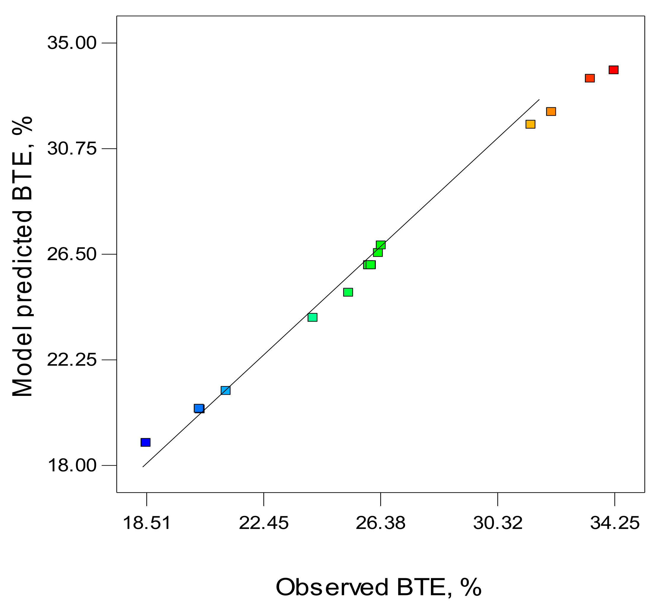
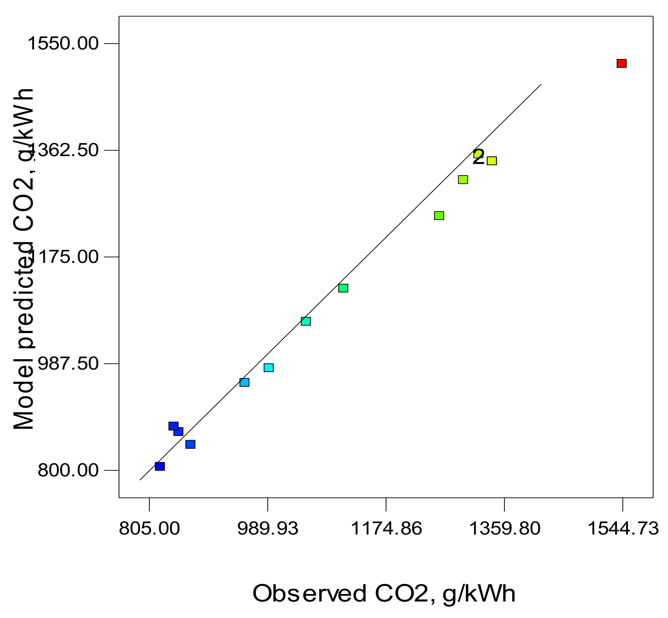
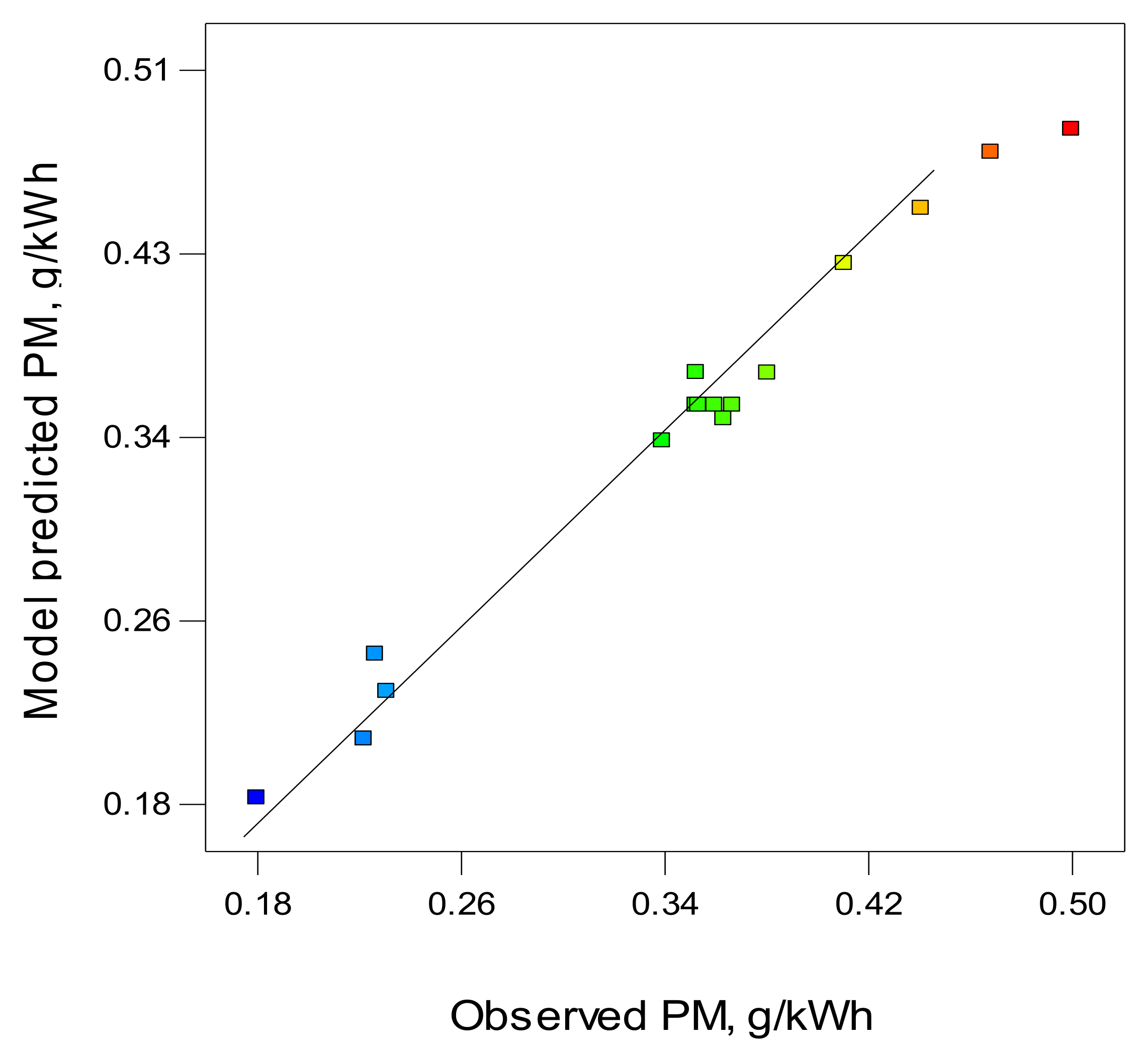
3.1. Predictive Model Evaluation

3.1.1. Combustion and Performance Models

The mathematical equations, Equations (5)–(9) developed with MORSM were used to predict the engine outputs for all engine trial runs. Table 7 shows the observed and MORSM predicted values of performance metrics such as BTE and BSFC. For model error analysis, these values were employed. A comparative presentation of observed and model-predicted BTE values is illustrated in Figure 2. BTE model could achieve the R and R2 values as 0.9989 and 0.9975, respectively. Both MAPD and RMSE were quite low for the BTE model. The predictive efficiency for the BTE model was measured with NSE as 0.9988. Similarly, the R and R2 for MORSM based BSFC model were 0.9917 and 0.9836, respectively. Figure 3 illustrates the comparison of model-predicted and observed BSFC values. The MAPD and RMSE for the BSFC model were 2.3% and 10.78 absolute. The NSE value for the BSFC model was 0.984. The proposed model’s superior prediction performance is demonstrated by its high correlation values (R and R2) and low model errors. Both the performance models had low MAPD values, indicating a strong predictive model capable of reliably forecasting the outputs. The R, R2, NSE, MAPD, and RMSE values for BTE and BSFC are listed in Table 8. Overall, the MORSM approach was demonstrated in this study to be capable of building a trustworthy engine performance prediction model [36,37]. In Figure 2, Figure 3, Figure 4, Figure 5 and Figure 6, the blue, green, yellow, amber, red colors indicate the increasing values of variables in the same sequence. The blue color denotes lowest while red denotes the highest values.

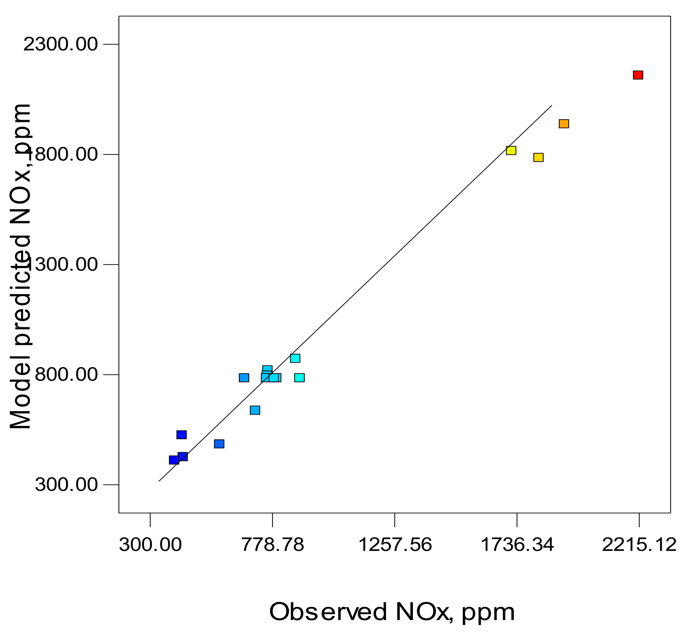
3.1.2. Engine Emission Characteristics Models

Emission models were developed for CO2, PM, and NOx using MORSM in the present work. The predictive models were used to forecast the emission characteristics values at different engine operating parameters. The MORSM based forecasted and observed values are compared in Figure 4, Figure 5 and Figure 6 for CO2, PM, and NOx, respectively. The observed and model-predicted values of NOx, H.C., and C.O. emissions are listed in Table 7. The present study analyzed the proposed models using statistical indices as mentioned in Equation (10) to Equation (12). The R-value denoting the correlation coefficient between observed and model forecasted values was 0.9969, 0.9820, and 0.9972 for CO2, PM, and NOx models, respectively. The coefficient of determination was predicted to be 0.9939, 0.9644, and 0.9944 for the proposed emission models of CO2, PM, and NOx, respectively. Both the correlation indices exhibit a superior degree of prediction ability. As estimated with NSE for CO2, PM, and NOx models, the efficiency of model prediction is 0.994, 0.965, and 0.9944, respectively. The MAPD (also known as MAPE) values were 1.2%, 4.4%, and 3.1% while RMSE was 17.29, 0.016, and 42.87 for CO2, PM, and NOx models, respectively. The low MAPD and RMSE values indicate an efficient prediction model. All the statistical indices estimated for emission models are listed in Table 8. The statistical indices demonstrate that MORSM is an efficient model prediction method [30,38].

3.1.3. Uncertainty Analysis of Predictive Models

Theil’s U1 and U2 values for the BTE model are 0.0042 and 0.0449, respectively, indicating that the proposed model is accurate and its predictive uncertainty is quite low. The model’s strong prognostic capacity with minimal uncertainty is demonstrated by these low numbers. BSFC also shows similar results, with U1 and U2 being 0.014 and 0.092, respectively. Theil’s U1 values for CO2, PM, and NOx emission models, respectively, are 0.0073, 0.022, and 0.019. Theil’s U2 for CO2, PM, and NOx emission models, respectively, is 0.059, 0.1804, and 0.125. Theil’s U1 and U2 values are very low, indicating that the MORSM-based prediction model is accurate and of good quality.

3.2. Interactive Effects of Control Variables on Response Factors

3.2.1. Brake Thermal Efficiency

The effects of control variables viz., engine load, compression ratio, and blending ratio on response factor (BTE) are illustrated in Figure 7. The common effect of compression ratio and engine load on BTE is illustrated in Figure 7a. It has been observed that engine load has a greater influence on BTE than compression ratio. The highest BTE was achieved to be closer to 80% of engine load and 17.5 of compression ratio. BTE improves with greater loads as the amount of fuel supplied increases and the engine’s breathing efficiency improves [39,40]. The interactive effects of blending ratio and engine load are shown in Figure 7b. Until now, increasing engine load has improved BTE, but blending ratio has had the reverse effect. With a larger blending ratio, the BTE progressively drops. The higher viscosity of biodiesel combined with the lower heating value of biodiesel is responsible for the loss in BTE at a higher blending ratio. Figure 7c illustrates the interaction of blending ratio and compression ratio. This substantiates the result of response surfaces shown in Figure 7a,b. Kashyap et al. [41] and Sharma [18] also present similar trends for BTE, showing that BTE is largely influenced by engine load and peak value of BTE is achieved close to 80% engine load.

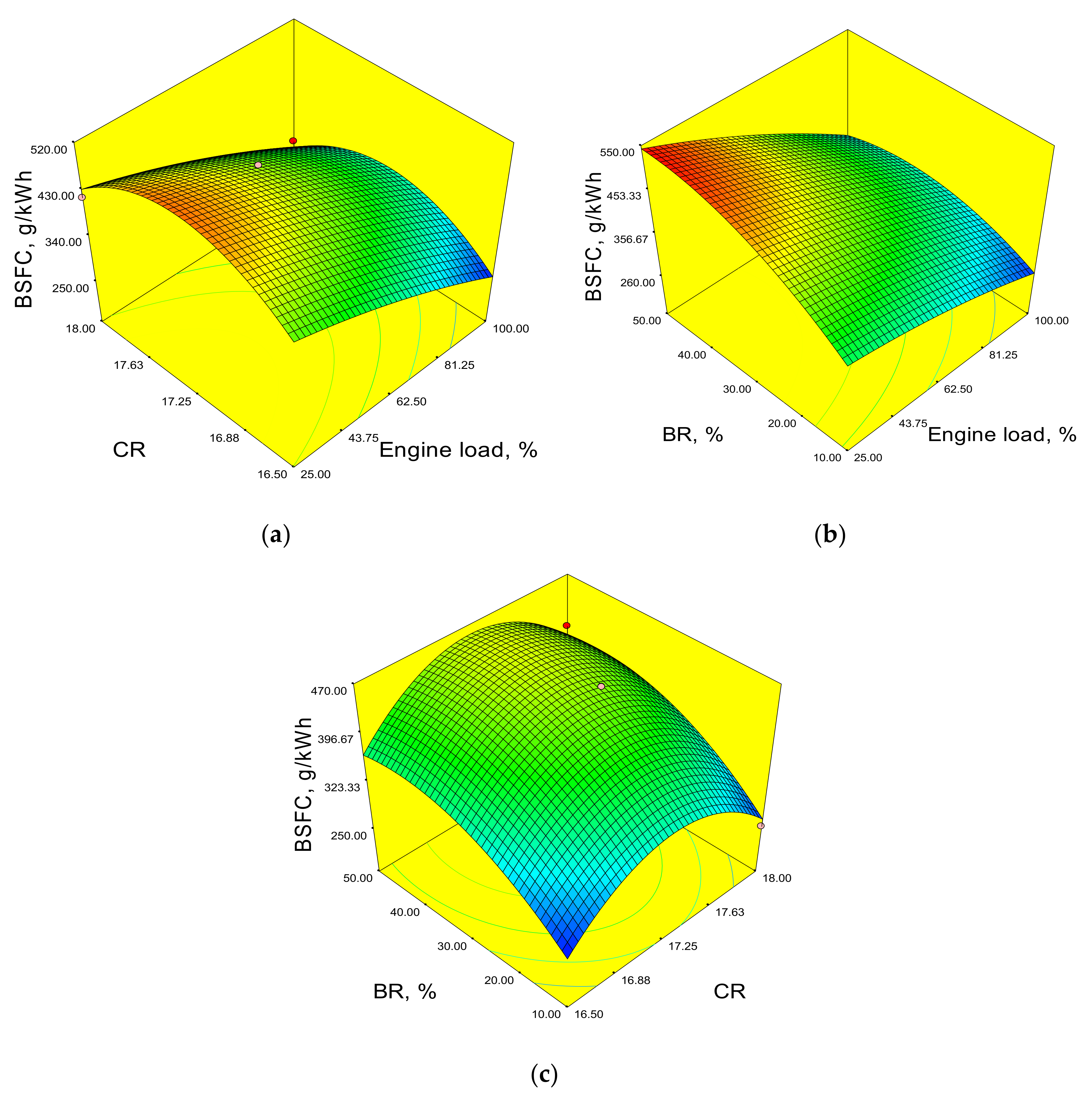
3.2.2. Brake Specific Fuel Consumption

The three-dimensional response surfaces depicting the impact of response variables on BSFC are shown in Figure 8. The combined effect of compression ratio and engine load, as shown in Figure 8a, demonstrates that BSFC initially increases with an increase in compression ratio and again reduces. The engine load on the other hand has a continuous positive effect on BSFC. The BSFC decreases with increasing engine load. The optimal BSFC can be observed at lower compression ratios but with higher engine load. These trends of BSFC are just opposite to BTE trends. The decreasing BSFC at higher engine load is the result of improved combustion and higher BTE [42]. The combined effect of engine load and blending ratio is shown in Figure 8b. It was observed that the lowest BSFC is observed at a lower blending ratio (close to 10%) and higher engine load (80% to 10%). Similarly, the interplay between compression ratio and blending mix is shown in Figure 8c. Minimum BSFC is observed between 17.5 to 18 compression ratio and 10% blending ratio. Uslu et al. [28] and Kataria et al. [43] also reported similar trends for BSFC under similar conditions, demonstrating that the lowest BSFC can be achieved at higher engine loads when combustion quality is superior.

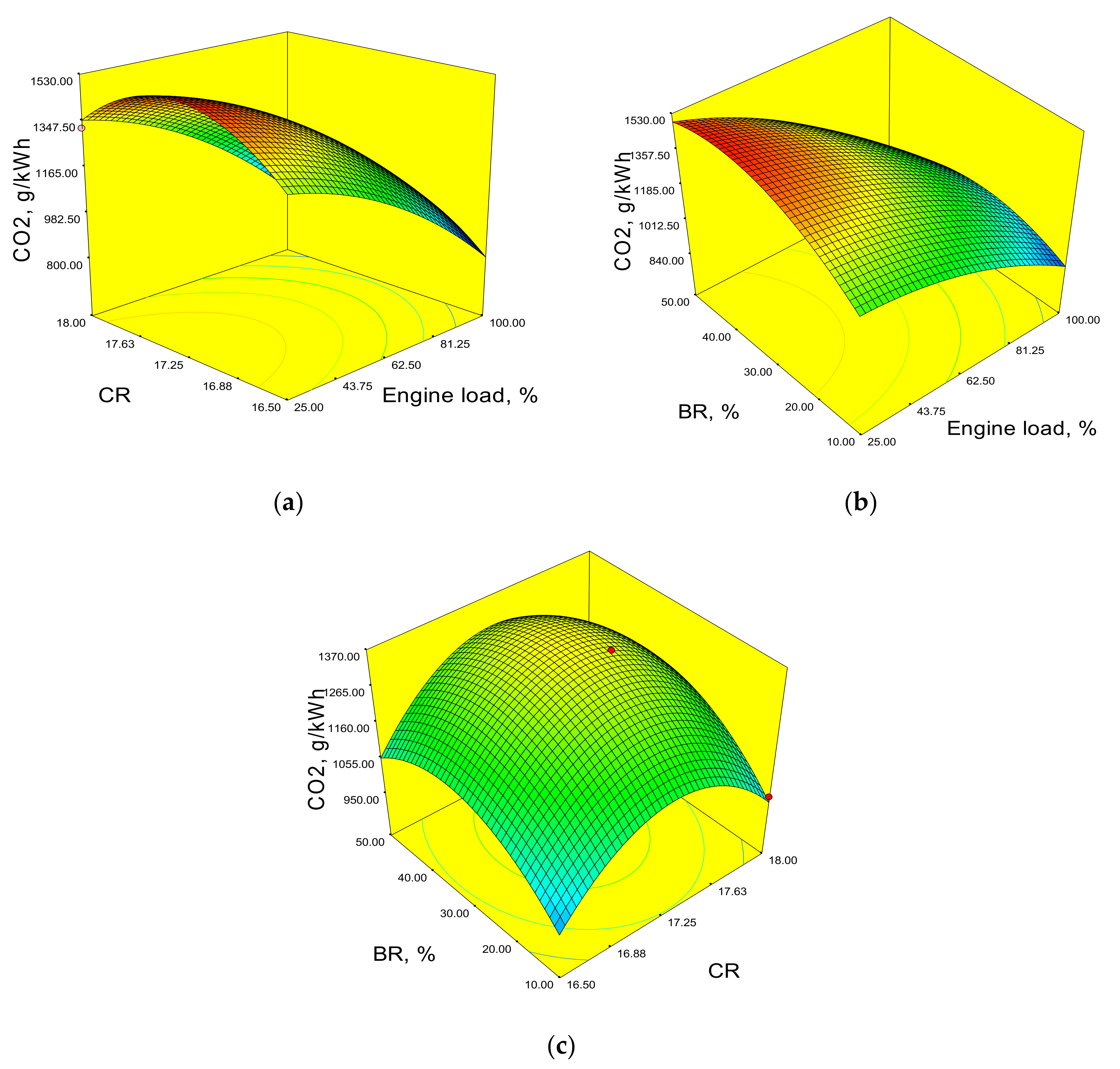
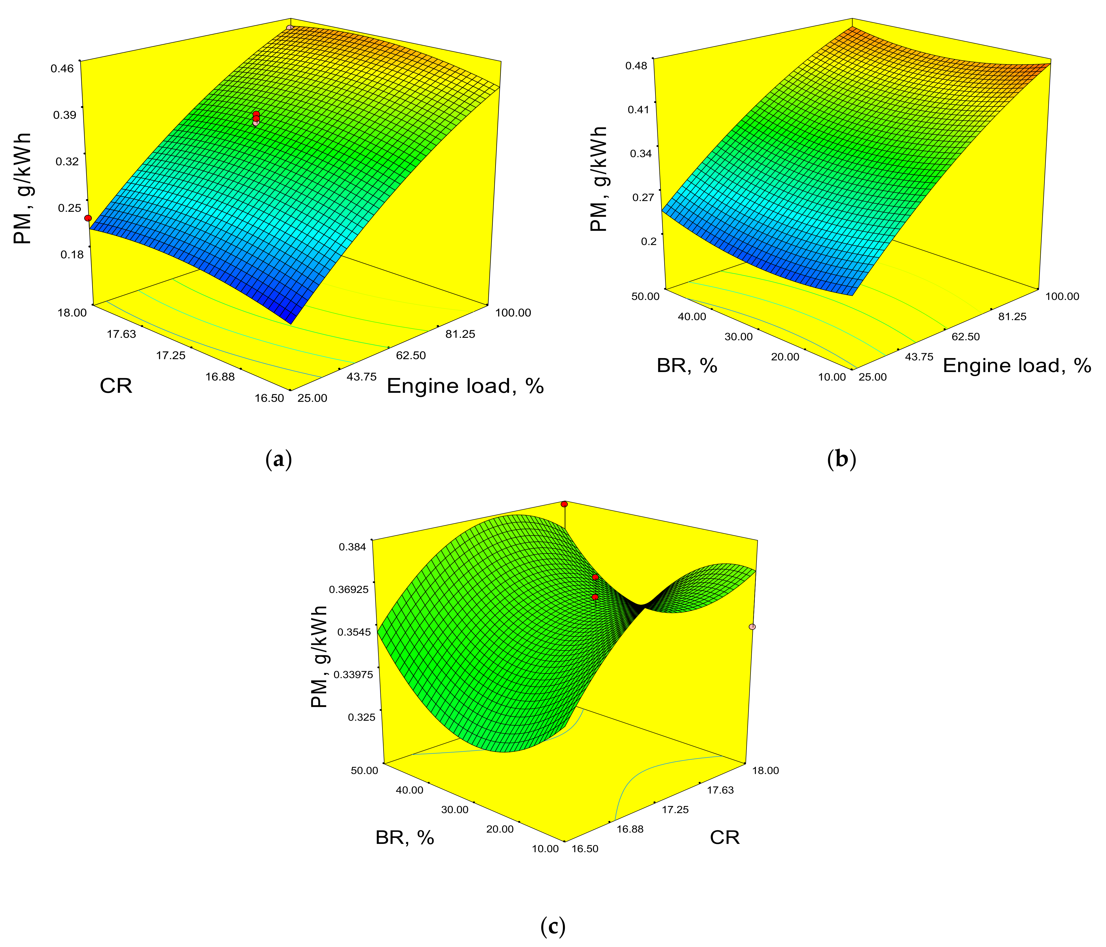
3.2.3. Exhaust Emission

The response surfaces depicting the combined impacts of engine load and compression ratio on CO2 exhaust emission are shown in Figure 9a. CO2 emissions appear to decrease as engine load increases, owing to better combustion at higher engine loads, as also reported in [13]. However, CO2 emission first increases then decreases on increasing the engine load. In terms of interaction, the lowest CO2 emission is observed to be between 80% and 10% engine load whilst the compression ratio is between 17.25 and 17.63. The interaction of engine load and biodiesel blending ratio is shown in Figure 9b. Figure 9c shows the combined impact of blending ratio and compression ratio predictions. It is observed that CO2 emission increases with the supply of a higher amount of biodiesel in blends, owing to the poorer combustion of algal biodiesel compared to diesel. Response surfaces make it easier to observe and understand the interplay of two control variables on one response variable [44].
The interactions of the control variables (engine load, compression ratio, and blending ratio) on PM emission are shown in Figure 10a–c. The interaction of load and compression ratio on PM emission is depicted in Figure 10a. It is observed that PM emission is mostly influenced by a change in engine load while the compression ratio has only a marginal effect on PM emission. Figure 10b predicts the combined effects of blending ratio and load. It is observed that initially, the PM emission decreases with an increase in blend ratio (higher biodiesel content) up to 28% but beyond this PM emission is observed to be increasing again. The PM emission in diesel engines increases due to poor combustion conditions. Figure 10c, depicts the combined effects of compression ratio and blending ratio. The lowest PM emission is observed between 20% and 30% biodiesel blends while the combined effect to produce lowest PM emission is observed at 18 compression ratio and 25% blending ratio. Sharma [21] and Billa et al. [30] also reported that engine load was the main influencing factor for the variation in PM emission.
Three-dimensional response surfaces are used to depict the cumulative impact of response variables on NOx emission (Figure 11). The collective impact of compression ratio and engine load on NOx emission is shown in Figure 11a. The interaction of blending ratio and engine load is depicted in Figure 11b. In both situations, NOx emission is minimal at low loads but increases with greater loads and a higher compression ratio [21]. The NOx increases at higher engine load owing to higher combustion temperatures. Figure 11c depicts the impact of blending ratio and compression ratio on NOx emission. Both appear to be canceling out each other’s effects, with the highest NOx emission in the response surface observed at a low compression ratio and with the 10% biodiesel blend. Kataria et al. [43] and Dubey et al. [45] also reported higher NOx at a higher compression ratio, especially at higher load owing to higher combustion temperature.

4. Optimization and Validation

4.1. Optimization Using Desirability Approach

Following the development of a robust predictive model, the optimization was performed to determine the optimal settings of control variables (input parameters) that produce the best response variables (output). To determine the best operating settings in MORSM, the desirability technique was employed. We can specify limitations in the desirability method, such as setting BTE to the maximum while setting emission and BSFC to minimal [41]. A bar graph illustrating individual and combined desirability is shown in Figure 12. At this level of desirability, the optimal engine operating conditions in terms of engine load, compression ratio, and biodiesel mixes were achieved. Table 9 lists both optimal operating conditions and forecasted output. The best control variables achieved in the present investigation are the engine load of 81.2%, the compression ratio of 17.5, and the biodiesel blending ratio of 10%. The MORSM projected value for BTE was 30.14%, while BSFC was 307.6 (g/kWh). The CO2, PM, and NOx emissions values were estimated as 1030.99 (g/kWh), 0.429 (g/kWh), and 1261.75 (ppm) at the optimized engine operating conditions.

4.2. Validation of Optimized Conditions

Lab-based tests were conducted to validate the MORSM model’s predictions for engine performance and emission characteristics. The engine was run at these optimum settings, and the performance and emission results were recorded. Table 9 shows the outcomes of an experiment carried out under optimal operating circumstances, as well as the percent departure from the model’s expected outputs. All of the experimental output was within 7.29% of the model-predicted values under optimal operating circumstances. The approach of validating the developed model through field studies was also exercised by Billa et al. [30] with an error range of 0.56–17.48%.

5. Conclusions

The performance of third-generation algal biodiesel was investigated in the present study using MORSM-based prognostic modeling. This approach improved upon the traditional practice of result presentation using one control factor and one response variable at a time. MORSM generated three-dimensional response surfaces that can present the interaction of two control variables on response variables, and their graphs are easy to interpret. In different ratios, Azolla pinnata oil methyl ester-diesel blends were used to power a variable compression engine at different engine load and compression ratios. The engine outputs, such as BTE, BSFC, CO2, PM, and NOx, were recorded at these diverse conditions. Using the Box–Behnken design and ANOVA, the input–output data were utilized to create five prediction models. Different recognized statistical metrics of error and efficiency analysis, such as R, R2, Nash–Sutcliffe efficiency, MAPD, and RMSE, were used to evaluate the prediction models. Theil’s U1 and U2 were computed to assess the accuracy and predictability of the created model. The desirability technique was used as a tool for analyzing combustion performance and emission trade-offs. The following are the conclusive outcomes of the present study:
  • With only 17 experimental tests, a reliable and efficient model was developed. It is noteworthy because three control variables and five response variables were employed at three levels.
  • The high R and R2 values (close to 1) achieved for all the prediction models with low prediction errors indicate an excellent degree of prediction ability of MORSM.
  • The generated model’s Nash–Sutcliffe efficiency was in the range of 0.965–0.9988, suggesting a stable model. In addition, the mean absolute percentage deviation was modest (0.7–4.4%).
  • The engine operating condition was optimized using the desirability technique. An optimum condition was reached with the engine load at 81.2%, compression ratio at 17.5, and with 10% biodiesel blends. The trade-off resulted in optimal combustion performance with low emission. The best performance output was obtained as 30.14% BTE, 307.36 g/kWh BSFC with exhaust emission CO2 as 1030.99 (g/kWh), PM as 0.429 (g/kWh), and NOx as 1261.75 ppm.
  • An experimental test was used to confirm the output anticipated under optimal conditions. The predictions were all within 7.29% of the experimental findings.
The present study is a successful endeavor to study third-generation algal biodiesel’s combustion and emission characteristics using MORSM based model prediction. The third-generation biodiesel feedstock does not affect the human food chain and is easier to produce. The study may further extend to dual-fuel engines and life cycle analysis to assess the potential environmental impacts.

Author Contributions

Conceptualization, P.S. and A.C.; methodology, P.S. and A.C.; software, P.S. and A.C.; validation, Z.S., P.S., and A.C.; formal analysis, P.S., A.C., and Z.S.; investigation, P.S. and A.C.; resources, P.S., A.C., Z.S., and S.M.; data curation, P.S., A.C., and Z.S.; writing—original draft preparation, P.S., A.C., Z.S., and S.M; writing—review and editing, S.M., Z.S., and P.S.; visualization, P.S. and A.C.; supervision, A.C. and Z.S.; project administration, P.S., A.C., Z.S., and S.M.; funding acquisition, P.S., A.C., Z.S., and S.M. All authors have read and agreed to the published version of the manuscript.

Funding

This work was supported by the international collaboration between the authors of this manuscript.

Institutional Review Board Statement

Not applicable.

Informed Consent Statement

Not applicable.

Data Availability Statement

Not applicable.

Acknowledgments

Authors thank Delhi Skill and Entrepreneurship University and corresponding international collaboration for working on this algal bio-diesel engine project. Zafar Said would like to thank the University of Sharjah, Projects #21020406162, for its financial support.

Conflicts of Interest

The authors declare no conflict of interest.

Abbreviations

AIArtificial intelligence
bTDCBefore top dead centre
BTEBrake thermal efficiency
CFDComputational fluid dynamics
GHGGreenhouse gas
MAPDMean absolute percentage deviation
NSENash-Sutcliffe Efficiency
SDGSustainable development goals
FFAFree fatty acid
FITFuel injection timing
ICEInternal combustion engine
ANNArtificial neural network
BSFCBrake specific fuel consumption
CO2Carbon dioxide
CRDiCommon rail direct injection
HCHydrocarbon
RMSERoot mean square error
NOxOxides of nitrogen
UNGAUnited nations general assembly
FIPFuel injection pressure
GEPGene expression programming
J/°CAJoule per crank angle

References

  1. Salvia, A.L.; Leal Filho, W.; Brandli, L.L.; Griebeler, J.S. Assessing research trends related to Sustainable Development Goals: Local and global issues. J. Clean. Prod. 2019, 208, 841–849. [Google Scholar] [CrossRef] [Green Version]
  2. Fuso Nerini, F.; Tomei, J.; To, L.S.; Bisaga, I.; Parikh, P.; Black, M.; Borrion, A.; Spataru, C.; Castán Broto, V.; Anandarajah, G.; et al. Mapping synergies and trade-offs between energy and the Sustainable Development Goals. Nat. Energy 2018, 3, 10–15. [Google Scholar] [CrossRef] [Green Version]
  3. Das, S.; Kashyap, D.; Kalita, P.; Kulkarni, V.; Itaya, Y. Clean gaseous fuel application in diesel engine: A sustainable option for rural electrification in India. Renew. Sustain. Energy Rev. 2020, 117, 109485. [Google Scholar] [CrossRef]
  4. Ong, H.C.; Tiong, Y.W.; Goh, B.H.H.; Gan, Y.Y.; Mofijur, M.; Fattah, I.M.R.; Chong, C.T.; Alam, M.A.; Lee, H.V.; Silitonga, A.S.; et al. Recent advances in biodiesel production from agricultural products and microalgae using ionic liquids: Opportunities and challenges. Energy Convers. Manag. 2021, 228, 113647. [Google Scholar] [CrossRef]
  5. Sansaniwal, S.K.; Pal, K.; Rosen, M.A.; Tyagi, S.K. Recent advances in the development of biomass gasification technology: A comprehensive review. Renew. Sustain. Energy Rev. 2017, 72, 363–384. [Google Scholar] [CrossRef]
  6. Atabani, A.E.; Silitonga, A.S.; Ong, H.C.; Mahlia, T.M.I.; Masjuki, H.H.; Badruddin, I.A.; Fayaz, H. Non-edible vegetable oils: A critical evaluation of oil extraction, fatty acid compositions, biodiesel production, characteristics, engine performance and emissions production. Renew. Sustain. Energy Rev. 2013, 18, 211–245. [Google Scholar] [CrossRef]
  7. Saad, M.G.; Dosoky, N.S.; Zoromba, M.S.; Shafik, H.M. Algal Biofuels: Current Status and Key Challenges. Energies 2019, 12, 1920. [Google Scholar] [CrossRef] [Green Version]
  8. Sharma, K.K.; Schuhmann, H.; Schenk, P.M. High Lipid Induction in Microalgae for Biodiesel Production. Energies 2012, 5, 1532–1553. [Google Scholar] [CrossRef] [Green Version]
  9. Ruiz-Marin, A.; Canedo-Lopez, Y.; Narvaez-Garcia, A.; Zavala-Loría, J.d.C.; Dzul-López, L.A.; Sámano-Celorio, M.L.; Crespo-Álvarez, J.; García-Villena, E.; Agudo-Toyos, P. Harvesting Scenedesmus obliquus via Flocculation of Moringa oleifera Seed Extract from Urban Wastewater: Proposal for the Integrated Use of Oil and Flocculant. Energies 2019, 12, 3996. [Google Scholar] [CrossRef] [Green Version]
  10. Jones, J.; Lee, C.-H.; Wang, J.; Poenie, M. Use of Anion Exchange Resins for One-Step Processing of Algae from Harvest to Biofuel. Energies 2012, 5, 2608–2625. [Google Scholar] [CrossRef]
  11. Jacob, A.; Ashok, B.; Alagumalai, A.; Chyuan, O.H.; Le, P.T.K. Critical review on third generation micro algae biodiesel production and its feasibility as future bioenergy for IC engine applications. Energy Convers. Manag. 2021, 228, 113655. [Google Scholar] [CrossRef]
  12. Czerwik-Marcinkowska, J.; Gałczyńska, K.; Oszczudłowski, J.; Massalski, A.; Semaniak, J.; Arabski, M. Fatty Acid Methyl Esters of the Aerophytic Cave Alga Coccomyxa subglobosa as a Source for Biodiesel Production. Energies 2020, 13, 6494. [Google Scholar] [CrossRef]
  13. Mubarak, M.; Shaija, A.; Suchithra, T.V. Experimental evaluation of Salvinia molesta oil biodiesel/diesel blends fuel on combustion, performance and emission analysis of diesel engine. Fuel 2021, 287, 119526. [Google Scholar] [CrossRef]
  14. Subramaniam, M.; Solomon, J.M.; Nadanakumar, V.; Anaimuthu, S.; Sathyamurthy, R. Experimental investigation on performance, combustion and emission characteristics of DI diesel engine using algae as a biodiesel. Energy Rep. 2020, 6, 1382–1392. [Google Scholar] [CrossRef]
  15. Nautiyal, P.; Subramanian, K.A.; Dastidar, M.G.; Kumar, A. Experimental assessment of performance, combustion and emissions of a compression ignition engine fuelled with Spirulina platensis biodiesel. Energy 2020, 193, 116861. [Google Scholar] [CrossRef]
  16. Gul, M.; Shah, A.N.; Aziz, U.; Husnain, N.; Abbas, M.; Kousar, T.; Ahmad, R.; Hanif, M.F. Grey-Taguchi and ANN based optimization of a better performing low-emission diesel engine fueled with biodiesel. Energy Sources, Part A Recover. Util. Environ. Eff. 2019, 1–14. [Google Scholar] [CrossRef]
  17. Sharma, P.; Sharma, A.K. AI-Based Prognostic Modeling and Performance Optimization of CI Engine Using Biodiesel-Diesel Blends. Int. J. Renew. Energy Resour. 2021, 11, 701–708. [Google Scholar]
  18. Sharma, P. Prediction-Optimization of the Effects of Di-Tert Butyl Peroxide-Biodiesel Blends on Engine Performance and Emissions Using Multi-Objective Response Surface Methodology (MORSM). J. Energy Resour. Technol. 2021, 144, 072301. [Google Scholar] [CrossRef]
  19. Sharma, P.; Sharma, A.K. Application of Response Surface Methodology for Optimization of Fuel Injection Parameters of a Dual Fuel Engine Fuelled with Producer Gas- Biodiesel blends. Energy Sources Part A Recover. Util. Environ. Eff. 2021, 1–18. [Google Scholar] [CrossRef]
  20. Ali, O.M.; Mamat, R.; Najafi, G.; Yusaf, T.; Mohammad, S.; Ardebili, S. Optimization of Biodiesel-Diesel Blended Fuel Properties and Engine Performance with Ether Additive Using Statistical Analysis and Response Surface Methods. Energies 2015, 8, 14136–14150. [Google Scholar] [CrossRef] [Green Version]
  21. Sharma, P. Gene expression programming-based model prediction of performance and emission characteristics of a diesel engine fueled with linseed oil biodiesel/diesel blends: An artificial intelligence approach. Energy Sources Part A Recover. Util. Environ. Eff. 2020, 2020, 1–15. [Google Scholar] [CrossRef]
  22. Sharma, P. Artificial intelligence-based model prediction of biodiesel-fueled engine performance and emission characteristics: A comparative evaluation of gene expression programming and artificial neural network. Heat Transf. 2021, 50, 5563–5587. [Google Scholar] [CrossRef]
  23. Said, Z.; Sharma, P.; Syam Sundar, L.; Afzal, A.; Li, C. Synthesis, stability, thermophysical properties and AI approach for predictive modelling of Fe3O4 Coated MWCNT Hybrid Nanofluids. J. Mol. Liq. 2021, 2021, 117291. [Google Scholar] [CrossRef]
  24. Bietresato, M.; Caligiuri, C.; Bolla, A.; Renzi, M.; Mazzetto, F. Proposal of a Predictive Mixed Experimental-Numerical Approach for Assessing the Performance of Farm Tractor Engines Fuelled with Diesel-Biodiesel-Bioethanol Blends. Energies 2019, 12, 2287. [Google Scholar] [CrossRef] [Green Version]
  25. Elkelawy, M.; Alm-Eldin Bastawissi, H.; El Shenawy, E.A.; Taha, M.; Panchal, H.; Sadasivuni, K.K. Study of performance, combustion, and emissions parameters of DI-diesel engine fueled with algae biodiesel/diesel/n-pentane blends. Energy Convers. Manag. X 2021, 10, 100058. [Google Scholar] [CrossRef]
  26. Murugapoopathi, S.; Vasudevan, D. Experimental and numerical findings on VCR engine performance analysis on high FFA RSO biodiesel as fuel using RSM approach. Heat Mass Transf. Stoffuebertragung 2021, 57, 495–513. [Google Scholar] [CrossRef]
  27. Hussain, S.A.I.; Sen, B.; Das Gupta, A.; Mandal, U.K. Novel Multi-objective Decision-Making and Trade-Off Approach for Selecting Optimal Machining Parameters of Inconel-800 Superalloy. Arab. J. Sci. Eng. 2020, 45, 5833–5847. [Google Scholar] [CrossRef]
  28. Simsek, S.; Uslu, S. Investigation of the effects of biodiesel/2-ethylhexyl nitrate (EHN) fuel blends on diesel engine performance and emissions by response surface methodology (RSM). Fuel 2020, 275, 118005. [Google Scholar] [CrossRef]
  29. Elkelawy, M.; Bastawissi, H.A.E.; Esmaeil, K.K.; Radwan, A.M.; Panchal, H.; Sadasivuni, K.K.; Suresh, M.; Israr, M. Maximization of biodiesel production from sunflower and soybean oils and prediction of diesel engine performance and emission characteristics through response surface methodology. Fuel 2020, 266, 117072. [Google Scholar] [CrossRef]
  30. Billa, K.K.; Sastry, G.R.K.; Deb, M. Characterization of emission-performance paradigm of a DI-CI engine using artificial intelligent based multi objective response surface methodology model fueled with diesel-biodiesel blends. Energy Sources Part A Recover. Util. Environ. Eff. 2020, 2020, 1–30. [Google Scholar] [CrossRef]
  31. Bhowmik, S.; Paul, A.; Panua, R.; Ghosh, S.K.; Debroy, D. Artificial intelligence based gene expression programming (GEP) model prediction of Diesel engine performances and exhaust emissions under Diesosenol fuel strategies. Fuel 2019, 235, 317–325. [Google Scholar] [CrossRef]
  32. Madheshiya, A.K.; Vedrtnam, A. Energy-exergy analysis of biodiesel fuels produced from waste cooking oil and mustard oil. Fuel 2018, 214, 386–408. [Google Scholar] [CrossRef]
  33. Syam Sundar, L.; Said, Z.; Saleh, B.; Singh, M.K.; Sousa, A.C.M. Combination of Co3O4 deposited rGO hybrid nanofluids and longitudinal strip inserts: Thermal properties, heat transfer, friction factor, and thermal performance evaluations. Therm. Sci. Eng. Prog. 2020, 20, 100695. [Google Scholar] [CrossRef]
  34. Dey, S.; Reang, N.M.; Majumder, A.; Deb, M.; Das, P.K. A hybrid ANN-Fuzzy approach for optimization of engine operating parameters of a CI engine fueled with diesel-palm biodiesel-ethanol blend. Energy 2020, 202, 117813. [Google Scholar] [CrossRef]
  35. Bhowmik, S.; Panua, R.; Ghosh, S.K.; Paul, A.; Debroy, D. Prediction of performance and exhaust emissions of diesel engine fuelled with adulterated diesel: An artificial neural network assisted fuzzy-based topology optimization. Energy Environ. 2018, 29, 1413–1437. [Google Scholar] [CrossRef]
  36. Iqbal, M.F.; Liu, Q.F.; Azim, I.; Zhu, X.; Yang, J.; Javed, M.F.; Rauf, M. Prediction of mechanical properties of green concrete incorporating waste foundry sand based on gene expression programming. J. Hazard. Mater. 2020, 384, 121322. [Google Scholar] [CrossRef] [PubMed]
  37. Said, Z.; Sundar, L.S.; Rezk, H.; Nassef, A.M.; Chakraborty, S.; Li, C. Thermophysical properties using ND/water nanofluids: An experimental study, ANFIS-based model and optimization. J. Mol. Liq. 2021, 330, 115659. [Google Scholar] [CrossRef]
  38. Kakati, D.; Roy, S.; Banerjee, R. Development and validation of an artificial intelligence platform for characterization of the exergy-emission-stability profiles of the PPCI-RCCI regimes in a diesel-methanol operation under varying injection phasing strategies: A Gene Expression Programming approach. Fuel 2021, 299, 120864. [Google Scholar] [CrossRef]
  39. Esonye, C.; Onukwuli, O.D.; Ofoefule, A.U.; Ogah, E.O. Multi-input multi-output (MIMO) ANN and Nelder-Mead’s simplex based modeling of engine performance and combustion emission characteristics of biodiesel-diesel blend in CI diesel engine. Appl. Therm. Eng. 2019, 151, 100–114. [Google Scholar] [CrossRef]
  40. Sharma, P.; Sharma, A.K. Experimental Evaluation of Thermal and Combustion Performance of a DI Diesel Engine Using Waste Cooking Oil Methyl Ester and Diesel Fuel Blends. In Proceedings of the Smart Innovation, Systems and Technologies, International Conference on Mechanical and Energy Technologies (ICMET-2019), Noida, India, 7–8 November 2019; Yadav, S., Singh, D.B., Arora, P.K., Kumar, H., Eds.; Springer: Singapore, 2020; Volume 174, pp. 551–559. [Google Scholar]
  41. Kashyap, D.; Das, S.; Kalita, P. Exploring the efficiency and pollutant emission of a dual fuel CI engine using biodiesel and producer gas: An optimization approach using response surface methodology. Sci. Total Environ. 2021, 773, 145633. [Google Scholar] [CrossRef]
  42. Wei, L.; Cheng, R.; Mao, H.; Geng, P.; Zhang, Y.; You, K. Combustion process and NOx emissions of a marine auxiliary diesel engine fuelled with waste cooking oil biodiesel blends. Energy 2018, 144, 73–80. [Google Scholar] [CrossRef]
  43. Kataria, J.; Mohapatra, S.K.; Kundu, K. Biodiesel production from waste cooking oil using heterogeneous catalysts and its operational characteristics on variable compression ratio CI engine. J. Energy Inst. 2019, 92, 275–287. [Google Scholar] [CrossRef]
  44. Mäkelä, M. Experimental design and response surface methodology in energy applications: A tutorial review. Energy Convers. Manag. 2017, 151, 630–640. [Google Scholar] [CrossRef]
  45. Dubey, P.; Gupta, R. Influences of dual bio-fuel (Jatropha biodiesel and turpentine oil) on single cylinder variable compression ratio diesel engine. Renew. Energy 2018, 115, 1294–1302. [Google Scholar] [CrossRef]
Figure 1. Schematic diagram of the experimental setup.
Energies 14 05968 g001
Figure 2. Observed vs. MORSM predicted BTE (%).
Energies 14 05968 g002
Figure 3. Observed vs. predicted BSFC (g/kWh).
Energies 14 05968 g003
Figure 4. Observed vs. predicted CO2 (g/kWh).
Energies 14 05968 g004
Figure 5. Observed and predicted PM (g/kWh).
Energies 14 05968 g005
Figure 6. Observed and predicted NOx (ppm).
Energies 14 05968 g006
Figure 7. Input parameters interaction surfaces for BTE (a) Compression ratio vs. engine load (b) blending ratio vs. engine load (c) blending ratio vs. compression ratio.
Energies 14 05968 g007
Figure 8. Input parameters interaction surfaces for BSFC (a) Compression ratio vs. engine load (b) blending ratio vs. engine load (c) blending ratio vs. compression ratio.
Energies 14 05968 g008
Figure 9. Input parameters interaction surfaces for CO2 (a) Compression ratio vs. engine load (b) blending ratio vs. engine load (c) blending ratio vs. compression ratio.
Energies 14 05968 g009
Figure 10. Input parameters interaction surfaces for PM (a) Compression ratio vs. engine load (b) blending ratio vs. engine load (c) blending ratio vs. compression ratio.
Energies 14 05968 g010
Figure 11. Input parameters interaction surfaces for NOx (a) Compression ratio vs. engine load (b) blending ratio vs. engine load (c) blending ratio vs. compression ratio.
Energies 14 05968 g011
Figure 12. Bar graph for desirability.
Energies 14 05968 g012
Table 1. Technical indices, test set up.
ParameterSpecification
Engine type and makeVariable compression ratio, Kirloskar
Loading unitEddy current dynamometer type
Dynamometer coolingWater
Size and capacity87.5 × 110 mm, 661 cm3
Engine Compression ratio12–18
Power rating3.5 kW @ 1500 rpm
Load sensorStrain gauge type
Temperature measurementThermocouple type k, and RTD
Water flow measurementTwo rotameters
Airflow measurementOrifice meter with air box
Table 2. Fuel characteristics.
CharacteristicsUnitDieselAlgal Biodiesel
Pour point°C−18−13
Density (15 °C)kg/m3834863
Cloud point°C ×12
LCVMJ/kg43.6241.14
Cetane index-4955
Fire point, °C°C76146
Kinematic viscosity, @ 20 °CcST3.514.91
Table 3. Design matrix considering the control factors and response variables.
Run No.Control FactorsResponse Variables
Engine Load (%)Compression RatioBlending Ratio (%)BTE (%)BSFC (g/kWh)CO2 (g/kWh)Particulate Matter (g/kWh)NOx (ppm)
525.0017.5010.0021.21400.391259.630.23574.80
1162.5016.5050.0024.13372.591051.330.36872.20
1362.5017.5030.0025.99437.401341.930.37889.20
962.5016.5010.0026.33252.10955.360.34763.30
1062.5018.0010.0026.42253.40993.240.35761.20
1762.5017.5030.0026.01438.001342.000.35758.20
1562.5017.5030.0026.0437.301341.810.36798.10
4100.0018.0030.0033.45283.94870.990.441825.10
8100.0017.5050.0031.46302.04852.180.471718.40
6100.0017.5010.0034.25268.47844.540.501925.10
1662.5017.5030.0026.09437.501341.900.36788.40
2100.0016.5030.0032.15268.38823.240.412215.10
325.0018.0030.0020.33418.531320.810.22427.60
1462.5017.5030.0026.08437.401341.930.36672.10
725.0017.5050.0018.51547.441544.720.23431.90
125.0016.5030.0020.30422.741296.930.18398.20
1262.5018.0050.0025.33393.331109.840.38715.30
Table 4. Experimental uncertainties parameters.
Measured
Parameter
RangeAccuracyUncertainty
Load0–50 kg±1 kg±0.02%
Temperature0–900 °C±°C±0.15
Speed0–10,000 rpm±10 rpm±1%
Fuel flow1–30 cc±0.1 cc±0.5%
CO20 to 20% by volume±0.03 Vol%±0.2%
PM0 to 20,000 ppm±0.01 Vol%±0.2%
NOx0 to 5000 ppm±1 ppm±0.1%
Calculated Parameter Uncertainty
BTE----±1.2%
BSFC----±0.8%
BP----±1.12%
Table 5. ANOVA outcomes for BTE and BSFC models.
ParameterBTEBSFC
Model
Source
F-Valuep-Value
Prob > F
F-Valuep-Value
Prob > F
Model338.01<0.0001118,697.6<0.0001
X-Load302.83<0.000138,195.36<0.0001
Y-CR0.86400.030517,479.06<0.0001
Z-BR9.66<0.000116,066.810.0001
XY0.49180.08076.020.8877
XZ0.00260.88733219.4280.0116
YZ0.12920.33058.9288530.8635
X21.860.0054789.84110.1373
Y20.00440.853121,803.59<0.0001
Z20.4987<0.00018240.2820.0010
Table 6. ANOVA outcomes for CO2, PM, NOx models.
ParameterCO2PMNOx
Model
Source
F-Valuep-Value
Prob > F
F-Valuep-Value
Prob > F
F-Valuep-Value
Prob > F
Model8.377 × 105<0.00010.122003<0.00015.116 × 106<0.0001
X-Load4.889 × 105<0.00010.077988<0.00014.295 × 106<0.0001
Y-CR3528.000.06330.0030780.010733,741.530.1039
Z-BR29,047.490.00045.8 × 10−50.64995538.130.4737
XY11.110.90507.46 × 10−70.958662,972.260.0379
XZ19,243.240.00130.0001830.42761018.570.7549
YZ273.900.55852.69 × 10−50.756311,852.690.3047
X229,036.730.00040.002240.02157.076 × 105<0.0001
Y21.2 × 105<0.00010.0010570.082755.360.9418
Z275157.45<0.00010.0020920.02483442.600.5694
Table 7. Actual experimental and model predicted values.
BTE (%)BSFC (g/kWh)CO2(g/kWh)PM (g/kWh)NOx (ppm)
Obs.Pred.ObsPred.Obs.Pred.Obs.Pred.Obs.Pred.
21.2120.97400.39379.371259.631245.570.230.25574.80571.21
24.1323.92372.59368.811051.331060.210.360.33872.20868.93
25.9926.04437.40437.521341.931341.910.370.35889.20882.22
26.3326.52252.10258.55955.36952.670.340.34763.30816.96
26.4226.83253.40266.90993.24978.560.350.35761.20763.04
26.0126.04438.00437.521342.001341.910.350.35758.20761.22
26.026.04437.30437.521341.811341.910.360.35798.10781.22
33.4533.54283.94269.29870.99843.750.440.451825.101821.22
31.4631.69302.04323.06852.18866.240.470.481718.401812.99
34.2533.88268.47269.54844.54875.950.500.491925.101934.22
26.0926.04437.50437.521341.901341.910.360.35788.40781.22
32.1532.20268.38260.94823.24805.000.410.432215.102210.35
20.3320.23418.53435.851320.811354.250.220.21427.60434.96
26.0826.04437.40437.521341.931341.910.360.35672.10781.22
18.5118.89547.44546.371544.721513.300.230.24431.90422.81
20.3020.26422.74427.511296.931309.000.180.19398.20407.59
25.3324.93393.33377.161109.841118.320.380.34715.30633.08
Table 8. Statistical evaluation of predictive models.
IndicesBTEBSFCCO2PMNOx
R0.99890.99170.99690.98200.9972
R20.99750.98360.99390.96440.9944
MAPD0.7%2.3%1.2%4.4%3.1%
NSE0.99880.9840.9940.9650.9944
RMSE0.2210.7817.290.01642.87
Theil’s U10.00420.0140.00730.0220.019
Theil’s U20.04490.0920.0590.18040.125
Table 9. MORSM Optimized operating condition, prediction, validation, and % error.
Optimized Control
Factors
Outputs
Engine LoadCRB Ratio BTEBSFCCO2PMNOx
81.2%17.510%Pred. results30.14
(%)
307.36
(g/kWh)
1030.
99(g/kWh)
0.42
9(g/kWh)
1261.75
(ppm)
Exp. output30.36
(%)
302.45
(g/kWh)
1051.25
(g/kWh)
0.411
(g/kWh)
1287.4
(ppm)
%Error7.29%1.6%1.96%4.19%2.03%
Publisher’s Note: MDPI stays neutral with regard to jurisdictional claims in published maps and institutional affiliations.

