Abstract
To accelerate the integration of fluctuating renewable energy technologies in the power systems, it is necessary to increase the flexibility of hydropower by operating turbines at off-design conditions. Unfortunately, this strategy causes deleterious flow phenomena such as von Kármán’s vortices at the wake of the vanes and/or blades. When their shedding frequency lies in the vicinity of a structure’s natural frequency, lock-in occurs and vibration amplitudes increase significantly. Moreover, if cavitation occurs at the centers of these vortices, the structure’s dynamic response will be modified. In order to understand this interaction and to avoid its negative consequences, the vibration behavior of a NACA 0009 hydrofoil under a torsional lock-in condition was numerically simulated for cavitation-free and cavitating-flow conditions. The results showed that the presence of vortex cavitation modified the formation and growth process of shed von Kármán vortices in the near-wake region which, in turn, caused an increase of the work performed by the hydrofoil deformation on the surrounding flow and a sharp decrease of the maximum vibration amplitude under resonance conditions.
1. Introduction
The introduction of intermittent and unpredictable energy sources, such as wind and solar power, compromises the stability of the electrical grid and leads hydroelectric turbines to work for longer periods of time at non-optimal operating points. These working conditions can cause complex flows, such as von Kármán’s vortices, to appear along the hydraulic circuit, which can result in unwanted periodic excitation forces.
Vortex shedding behind solid bodies located in a fluid stream has attracted the attention of researchers since 1878, when Strouhal observed this phenomenon experimentally for the first time [1]. The vortex shedding is a consequence of the boundary layer detachment on both the upper and lower surfaces of the solid body. Above a critical Reynolds number, these detachments form a periodic array of discrete vortices referred to as von Karman’s vortex street [2,3,4,5]. Due to the asymmetric formation of these vortices, the body experiences an oscillating lift force [6].
When the oscillation frequency of the lift force lies in the vicinity of a body’s natural frequency, resonance can occur, which often results in potentially dangerous vibration amplitudes [7,8]. Vortex shedding as a mechanism of premature failure has been reported in a wide range of structures [9]. For instance, structural damage has specifically been observed on stay vanes and runner blades of hydraulic turbines, and is often attributed to severe fatigue loading [10,11,12,13,14]. It is therefore of paramount importance to predict the vibration amplitude of hydrofoils under resonance conditions in order to avoid catastrophic failures and to estimate their life expectancy.
As long as the hydrofoil is not under a resonance condition, the vortex shedding frequency varies linearly with the free stream velocity, often referred to as lock-off regime [1]. In the case of resonance, the vortex shedding frequency has a constant value for a specific range of free stream velocities, the so-called lock-in regime. It is observed that the lock-in of the vortex shedding frequency around a cantilever hydrofoil occurs for the first torsional mode [6].
Many researchers have focused their investigations on the prediction of the vortex shedding frequency. For instance, Vu et al. [15] first developed a numerical methodology to predict the von Kármán vortex shedding frequency of a turbine stay vane. They predicted the frequency using 2D unsteady flow simulations with the Shear Stress Transport (SST) turbulence model. The difference observed between the computed and the experimentally measured frequencies was about 18%. Nevertheless, Alexandre et al. [16] were not able to capture the vortex wake correctly with Unsteady Reynolds Averaged Navier Stokes (URANS) equations. They obtained more realistic results using the Detached Eddy Simulation (DES) model. Nowadays, the accuracy for the numerical computation of the vortex shedding frequency is about 10% [17].
When pressure falls below vapor pressure in a liquid, cavitation occurs. Due to the high vorticity taking place in the centers of the vortices, sharp decreases in pressure are expected to occur. As a result, these regions are more prone to develop vortex cavitation [18,19].
Both the vortex shedding frequency and vortex formation length have been observed to be sensitive to the extent of wake cavitation. For example, Young et al. [20] experimentally studied the vortex shedding frequency behind a 2D triangular wedge. They observed an increase in the frequency when wake cavitation was developed. Later, Belahadji et al. [21] also concluded that wake cavitation changed the flow dynamics and led to an increase in the vortex shedding frequency. Ausoni et al. [6] experimentally confirmed that the wake cavitation is responsible for the increase in the vortex shedding frequency behind a truncated NACA 0009 hydrofoil. Chen et al. [22] simulated the cavitating flow around a 2D NACA 0009 hydrofoil. They predicted an increase in the vortex shedding frequency of about 14% for a cavitation number around 40% of the incipient one.
Concerning the vortex formation length, Gerrard et al. [4] concluded that a larger vortex formation region leads to a decrease in the vortex frequency for single-phase flows. In the same direction, Ausoni et al. [6] reached the same conclusion after conducting experiments, again for cavitation-free regimes. Nevertheless, no experimental measurements were reported when cavitation occurred. On the other hand, Ramamurthy et al. [23] concluded that the higher the degree of the wake cavitation, the larger the vortex formation length. This conclusion was reached through experiments carried out on different geometries such as a cylinder and a two-dimensional triangular wedge. These results highlighted the fact that wake cavitation makes this phenomenon more complex.
The study of fluid-structure interaction (FSI) phenomena requires considering the flow behavior at the wake of hydrofoils and the structure dynamic response. In this sense, Zeng et al. [24] studied the dynamic response of the first bending mode of a blunt trailing-edge hydrofoil in a fluid stream through two-way FSI simulations. They concluded that this approach is suitable for the prediction of the vibration amplitude with a maximum deviation of around 8.82% for the hydrodynamic damping. Liaghat et al. [25] also studied the dynamic response of the first bending mode of a hydrofoil by using two-way FSI simulations. They numerically found the linear relationship between the hydrodynamic damping and the free-stream velocity. They reported that the deviation from experimentally obtained hydrodynamic damping ratios was around 12%. Like in the previous studies, Zeng et al. [26] numerically studied the dynamic response of a hydrofoil bending mode through two-way FSI simulations. They concluded that despite the usefulness of this approach, the numerical damping could induce uncertainty in the results. However, they also captured the linear dependency between the free-stream velocity and the hydrodynamic damping.
The prediction of hydrofoil vibration amplitudes under lock-in conditions has received far less attention than under lock-off conditions. In this sense, Alexandre et al. [27] studied the lift force, the vibration amplitude, and the frequency value of a hydrofoil under a lock-in condition. They modelled the torsional mode as a single degree of freedom system and coupled it to a CFD simulation. They concluded that this method can capture the increase of vibration amplitude in lock-in conditions. Miyagawa et al. [28] also modelled the resonant mode of vibration as a single degree of freedom oscillator. They included it in a CFD simulation in order to predict the vibration amplitudes in lock-in conditions. Additionally, they computed the hydrodynamic damping corresponding to different values of the reduced velocity. In particular, a decrease in the hydrodynamic damping was found when large amplitudes of vibration occurred. They concluded that the drop in the damping was a result of a self-excitation mechanism. Nennemann et al. [17] predicted the vibration amplitude of hydraulic profiles under a torsional lock-in regime through an alternative methodology usually referred to as modal work approach. This method was validated by comparing the numerically predicted and the experimentally measured maximum vibration amplitudes of two different hydrofoils under lock-in conditions. For a truncated NACA 0009 profile, the deviation of the simulation result was nearly 0%, while the vibration amplitude was about 30% over-predicted for the other hydrofoil. This discrepancy was attributed to either the existence of an acoustic damping or to the incorrect transposition from measured strains to displacements.
Most research has been focused on lock-in conditions for free wake cavitation regimes, whilst there is a lack of investigations when wake cavitation occurs with few available bibliography resources. For example, Ausoni et al. [6] experimentally studied the impact of the wake cavitation on the formation process of the vortex street. They concluded that wake cavitation should be considered as an active agent in the process since they observed a drop in the vibration amplitude of a hydrofoil under torsional lock-in conditions when wake cavitation occurred.
In summary, most of the literature related to the study of hydrofoils under vortex shedding flows deals with: (i) the prediction of the vortex shedding frequency for free-wake cavitation conditions [12,15,16,29,30,31,32], (ii) the influence of the wake cavitation on the vortex shedding dynamic behavior [4,20,21,22,23], and (iii) the prediction of the vibration amplitudes of hydrofoil under lock-off and lock-in conditions when no wake cavitation occurs [17,24,25,26,27,28]. However, solely Ausoni et al. [6] experimentally studied the interaction between wake cavitation and the dynamic response of a hydrofoil under a lock-in condition. For this reason, it is of paramount importance to conduct further research on this topic with the aim of predicting vibration amplitudes with good accuracy when wake cavitation occurs to understand the phenomena involved in the interaction between wake cavitation and lock-in conditions.
In the present article, the modal work approach proposed by Nennemann et al. [17] was firstly used to calculate the vibration modal amplitude of a NACA 0009 profile under a torsional lock-in condition and to assess its suitability not only for free-wake cavitation regimes, but also for incipient wake cavitation conditions. Secondly, the obtained results were analyzed to understand the mechanism responsible for the experimentally observed drop in the hydrofoil vibration amplitude when wake cavitation is developed.
The present paper starts with a review of studies on hydrofoils under vortex shedding flows. In the following section, a detailed explanation of the modal work approach applied to a NACA 0009 profile as well as an overview of the numerical model are provided. The results section is divided into, first, the validation of the numerical simulations, in which a comparison between experimental and numerical results is shown, and second, the discussion, in which the results employed to study the mechanism responsible for the drop in the vibration amplitude are presented. Finally, a summary of the most relevant findings is given in the conclusions.
2. Methodology
2.1. Modal Work Approach
Von Karman vortices formed on the trailing edge exert a dynamic loading on hydrofoils under lock-in conditions that transfer energy from the fluid to the vibrating structure in the form of work. On the other hand, the structural deformation and the displacement of the hydrofoil surfaces within the fluid domain can be also understood as another transfer of energy, but in this case from the structure to the fluid. According to the “Energy consideration” concept described by Naudascher et al. [7], the energy transfers from the structure to the fluid and from the fluid to the structure tend to be in balance for one cycle of vibration in a lock-in condition.
The idea of the modal work approach resides in finding the vibration amplitude which results in zero energy exchanged between the displacement of the structure within the flow and the surrounding fluid during one cycle of vibration. This calculation is carried out through an iterative process of simulations in which the hydrofoil surface’s periodic motion imposed in the CFD by an initial assumed modal amplitude is updated according to the value of the computed exchanged energy after each iteration until convergence to zero work is achieved.
Under lock-in conditions, the hydrofoil vibration oscillates periodically according to the mode shape of the excited resonance. In this case, the vector of surface displacements can be expressed as follows:
where is the displacement vector of the structural surface, is the normalized mode of vibration, q is the vibration modal amplitude, and the natural frequency of the mode.
It is noticeable that with the vibration modal amplitude, q, and the normalized mode shape, , the vibration amplitude of any point of the structural surface can be computed through Equation (1). Moreover, it can be seen that the maximum vibration amplitude of the structural surface is equal to q.
To reproduce the lock-in condition in the CFD simulation, , and an estimated modal amplitude, , are imposed in the solid boundary in order to define the hydrofoil surface periodic motion. Subsequently, the energy exchange between the structure and the fluid can be computed from:
where is the pressure, is the shear stress, is the velocity of the structure surface in the normal direction when vibrating under the resonant condition, and is the modal work performed by the structure on the fluid.
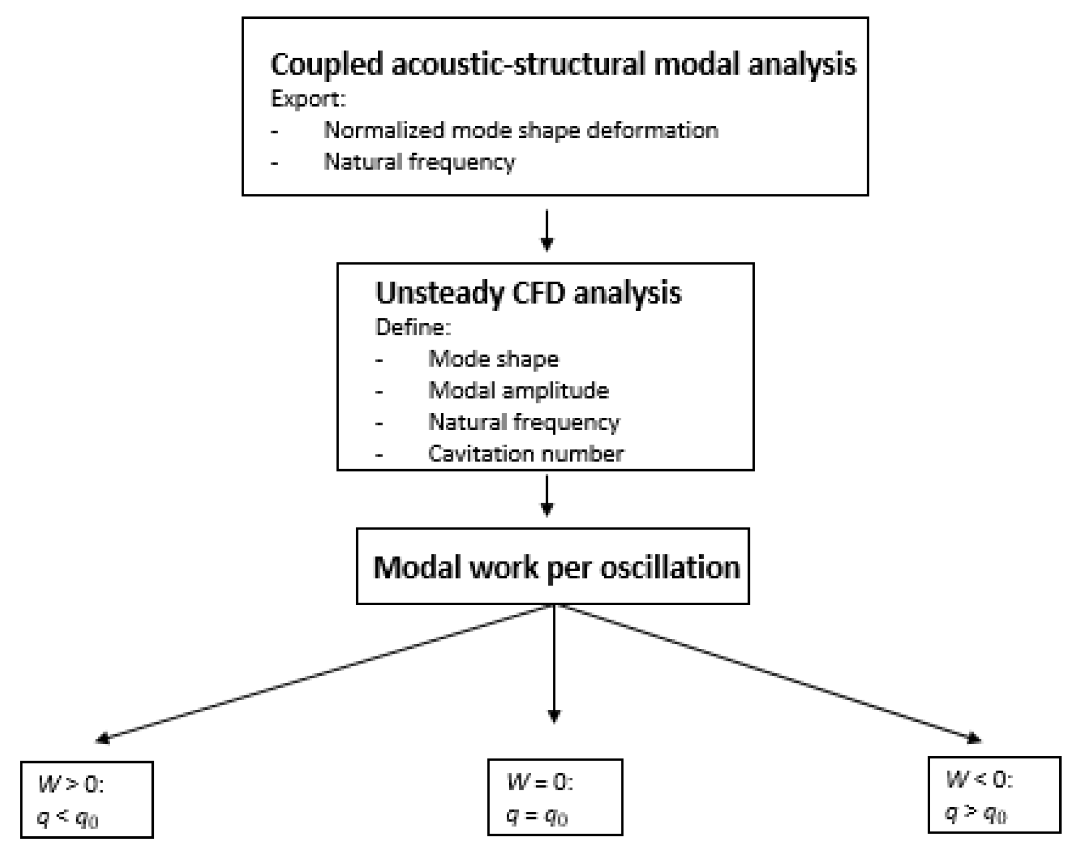
Based on the assumption described by Naudascher et al. [7], a positive value of W indicates that the needed vibration modal amplitude, q, is smaller than the estimated vibration modal amplitude, . Conversely, q is larger than if W is negative. In the case that W = 0, when q equals , the energy exchange is in balance and thus the lock-in condition is well characterized and simulated.
In the present work, the modal work approach was employed to calculate the vibration modal amplitudes, q, for no cavitation and incipient cavitation conditions in addition to studying the trend of q as a function of the cavitation number, deduced from the tendency of W.
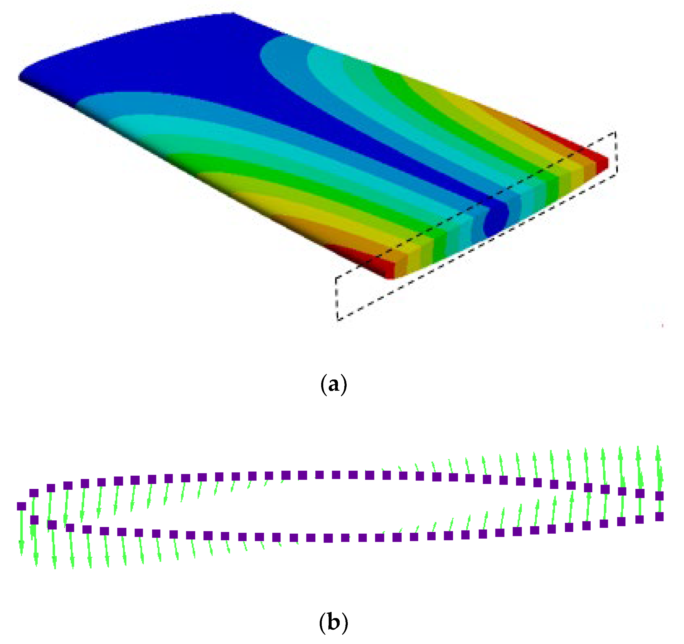
To begin with, the normalized mode shape, , and the natural frequency, , corresponding to the 3D torsion mode were determined through a coupled acoustic-structural modal analysis. This method accounts for the reduction of natural frequencies when structures are submerged in a dense fluid owing to the added mass effect. This methodology has been proven to give reasonably accurate results in the past [33,34,35]. The displacement of the hydrofoil in a section close to the tip, where the maximum displacement takes place, was then selected and imported in the CFD model as shown in Figure 1. The method has been tested with different 2D sections of the torsion mode and proven to be insensitive to displacement levels.

Figure 1.
(a) Normalized mode shape with the selected section highlighted in black and (b) the CFD model with the imported mode shape section.
Subsequently, the hydrofoil surface periodic motion was defined in a CFD simulation based on , and with an initially assumed vibration modal amplitude, . The corresponding boundary conditions were a uniform velocity at the inlet and an average static pressure at the outlet. Finally, from the CFD simulations, the modal work, W, was computed. A flow chart of the methodology is shown in Figure 2.
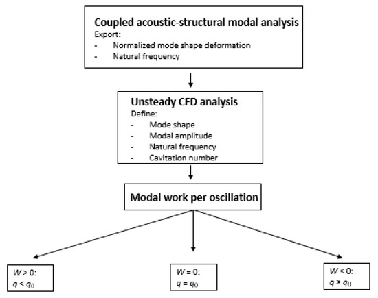
Figure 2.
Modal work computation flow chart.
On the one hand, in order to calculate the q corresponding to a specific cavitation condition, the average static pressure at the outlet of the flow was fixed in the CFD, while the assumed vibration modal amplitude, , was updated after each simulation. Specifically, the sign and value of W after each computation were considered to iterate a new value of , i.e., a positive W implies a reduction of whereas a negative W implies an increase of . This iterative process continued until reaching a , which results in W being approximately null. In this article, W was considered null when . W was divided by in order to eliminate its dependency on and to make possible the comparison of W/ between cases in which different were assumed.
On the other hand, in order to study the evolution of q as a function of the cavitation number, the assumed was fixed in the CFD whilst the average static pressure at the outlet of the flow was gradually reduced in a series of simulations, where W is calculated. Finally, from the tendency of W as a function of the cavitation number, the evolution of q can be deduced, i.e., an increase of W means that the variable q is reduced while a decrease in W means that it is increased.
2.2. Numerical Setup
The experimental results obtained by Ausoni et al. [6] were used as a reference for the present paper. These experiments were carried out with a NACA 0009 hydrofoil with chord length, c, and span, sp, of 100 and 150 mm, respectively, inside a rectangular test section with dimensions of 150 × 150 × 750 mm of the EPFL high-speed cavitation tunnel. They observed the lock-in of the first torsional mode of vibration at a free-stream velocity of about 12 m/s. The vortex-induced vibration for this condition was measured with a laser vibrometer located at a distance of 80 mm in the chordwise direction and 112.5 mm in the spanwise direction.
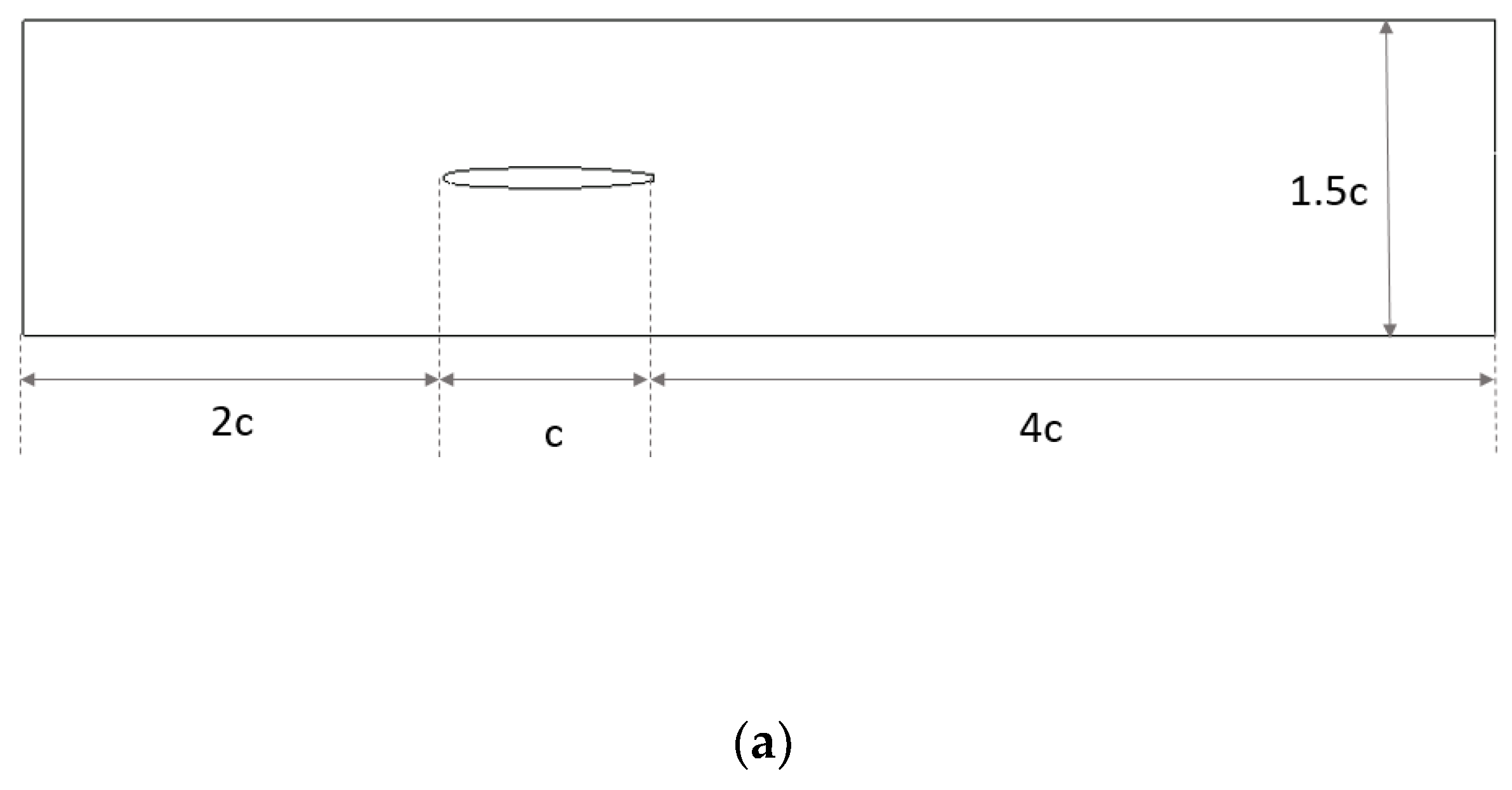
Figure 3 presents the dimensions and boundary conditions of the CFD domain corresponding to the lock-in condition observed experimentally by Ausoni et al. [6]. The top and bottom boundaries in addition to the hydrofoil surface were set with no slip wall condition. At the inlet, a uniform free-stream velocity of 12 m/s perpendicular to the inlet boundary with a 5% of turbulence intensity was imposed, whereas an average static pressure was employed at the outlet boundary. Symmetry conditions were considered at both lateral surfaces in the spanwise direction. This 2D assumption was previously applied with reasonable accuracy by Alexandre et al. [27] and Miyagawa et al. [28]. Finally, the hydrofoil surface periodic motion was defined through the torsion mode shape, a of 887.5 Hz corresponding to the torsion natural frequency, and an assumed .


Figure 3.
(a) Computational domain with dimensions and (b) scheme of the boundary conditions.
With regard to the turbulence modelling, the transition SST model was employed. For cavitation simulation, a homogeneous mixture model was considered which neglects the velocity differences between the liquid and the vapor phases by considering a single fluid with mixture properties. Thus, the mixture density and viscosity were calculated from a summation of their corresponding amounts in liquid and vapor states weighted by the volume fraction of each state, respectively. In particular, the Zwart-Gerber-Belamri cavitation mass transfer model was used to calculate the mass transfer rate between liquid and vapor and thus to derive the vapor volume fraction. In this model, the following parameters were considered: (i) a saturated vapor pressure of 2000 Pa, (ii) an initial value of the bubble radius of 1 µm, (iii) a nucleation site of the volume fraction of 0.0005, (iv) an empirical condensation coefficient of 0.01, and (v) an empirical vaporization coefficient of 50.
Regarding the solution methods, a time step of 0.000028 s was considered with the high-resolution advection scheme, the second-order backward Euler transient scheme, and the high-resolution turbulence numeric to solve the flow.
Under lock-in conditions, the vortex shedding frequency can be derived from the temporal evolution of the lift and the drag coefficients, CL and CD. The expressions used to calculate the CL and CD are presented as follows:
where is the water density, is the inlet velocity, is the reference area considered, is the fluid force perpendicular to the free-stream velocity, and is the force parallel to the free-stream velocity. Figure 4 shows an example of the time histories of the CL and CD for a cavitating condition.
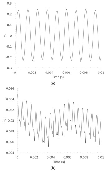
Figure 4.
Time histories of the CL (a) and CD (b) for the developed condition.
The validation of the grid independence was carried out under non-cavitating conditions and with four (4) different mesh refinement levels. Specifically, the vortex shedding frequency calculated from the time history of the lift coefficient was considered as the verification variable. The results obtained with the different refined meshes are listed in Table 1.

Table 1.
Details of the checked meshes and results obtained for the mesh independency study.
The grid convergence index (GCI) methodology was employed in order to verify that the solution was insensitive to the grid resolution [36]. In this case, the vortex shedding frequency was chosen as a parameter indicative of the grid convergence (ɸ). Both mesh refinement ratios, r21 and r43, being greater than 1.3, met the GCI requirements. Table 2 shows that the extrapolated value (ɸ31ext) was 882 Hz, the approximate relative error (ɸ31a_E) and the extrapolated relative error (ɸ31ext_E) were 2.2% and 0.68% respectively, and the GCI was 0.84%.
Table 2.
Results obtained for the variables of the GCI methodology.
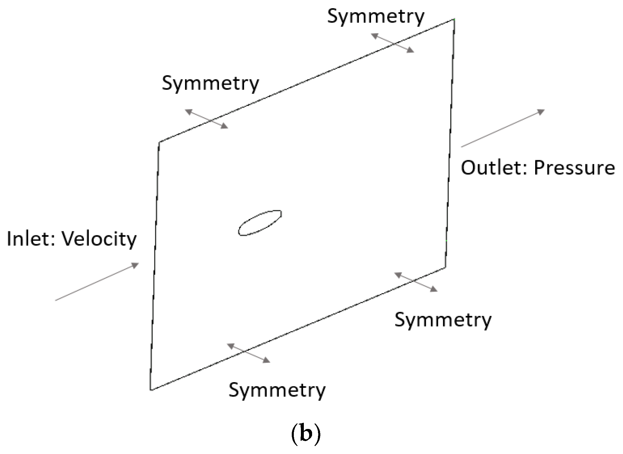
In Figure 5, the selected mesh (N1) as well as a detail of the trailing edge are presented:
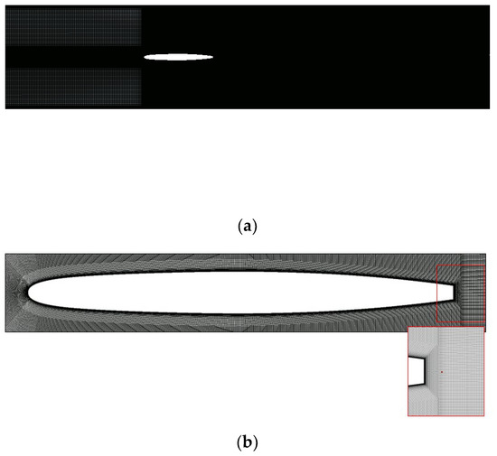
Figure 5.
(a) Selected mesh for the entire fluid domain (N1) and (b) detailed zooms showing the mesh topology around the hydrofoil surface and near the wake region.
The cavitation number is defined as follows:
where is the reference outlet pressure and is the vapor pressure.
The occurrence of the wake cavitation for the first time was identified numerically when the outlet absolute pressure was around 130,000 Pa based on the observation of: (i) vapor volume fractions higher than zero and (ii) pressure levels around the vapor pressure at the wake of the blade. This condition is referred to as cavitation incipient number, , and in the present paper it took a value of 1.77.
Table 3 presents the and the ratio of the cavitation number relative to the incipient cavitation number, , employed in the simulations. In the first simulation group (1), the hydrofoil surface periodic motion was not included in the CFD. In this case, the vortex shedding frequency was computed for different cavitation conditions with the objective of verifying whether the model accounts for the increase in the vortex shedding frequency when wake cavitation occurs. In the second (2) and third (3) simulation groups, the values of q corresponding to a wake-cavitation-free regime, , and to an incipient cavitation condition, , were calculated with an iterative process of simulations. During these computations, the suitability of the modal work approach in order to calculate vibration modal amplitudes was assessed. Finally, in the fourth simulation group (4), the q computed previously for was considered in a series of CFD simulations in which the cavitation number was gradually reduced. Then, from the evolution of the calculated W, the tendency of q as a function of the cavitation number was studied and thus also the mechanism responsible for the drop in the vibration modal amplitude when wake cavitation was developed.
Table 3.
Relative cavitation number and modal amplitudes.
3. Results
3.1. Validation of the CFD Model
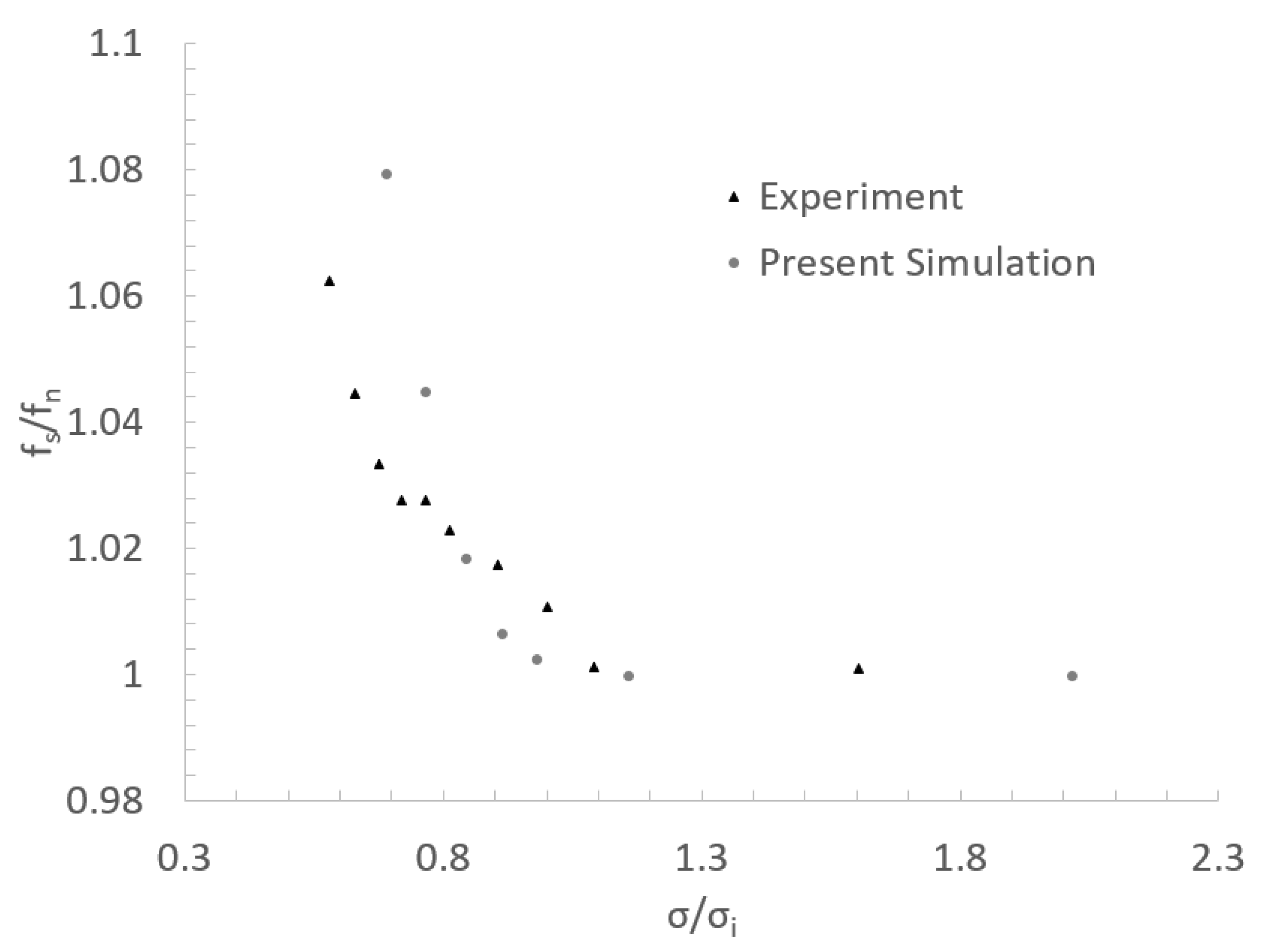
The vortex shedding frequencies obtained from the spectral analysis of the lift coefficient time series computed in the simulations of group (1), see Table 3, were compared with those measured experimentally by Ausoni et al. [6] in Figure 6.
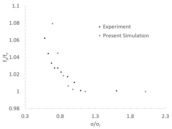
Figure 6.
Comparison of the vortex shedding frequencies estimates between the numerical simulations and the experimental measurements (Ausoni et al. [6]) as a function of the relative sigma value.
Figure 6 shows that both numerical and experimental vortex shedding frequencies were constant for higher than 1, whereas they sharply increased when fell below 1. It can be seen that the experimental vortex shedding frequencies increased faster than the numerical ones between 0.8 and 1. Nevertheless, this tendency was reversed for below 0.8. Overall, it can be considered that the numerical model used in the present work accounted for the phenomena responsible for the increase in the vortex shedding frequency when the cavitation number is decreased.
3.2. Validation of the Modal Work Approach
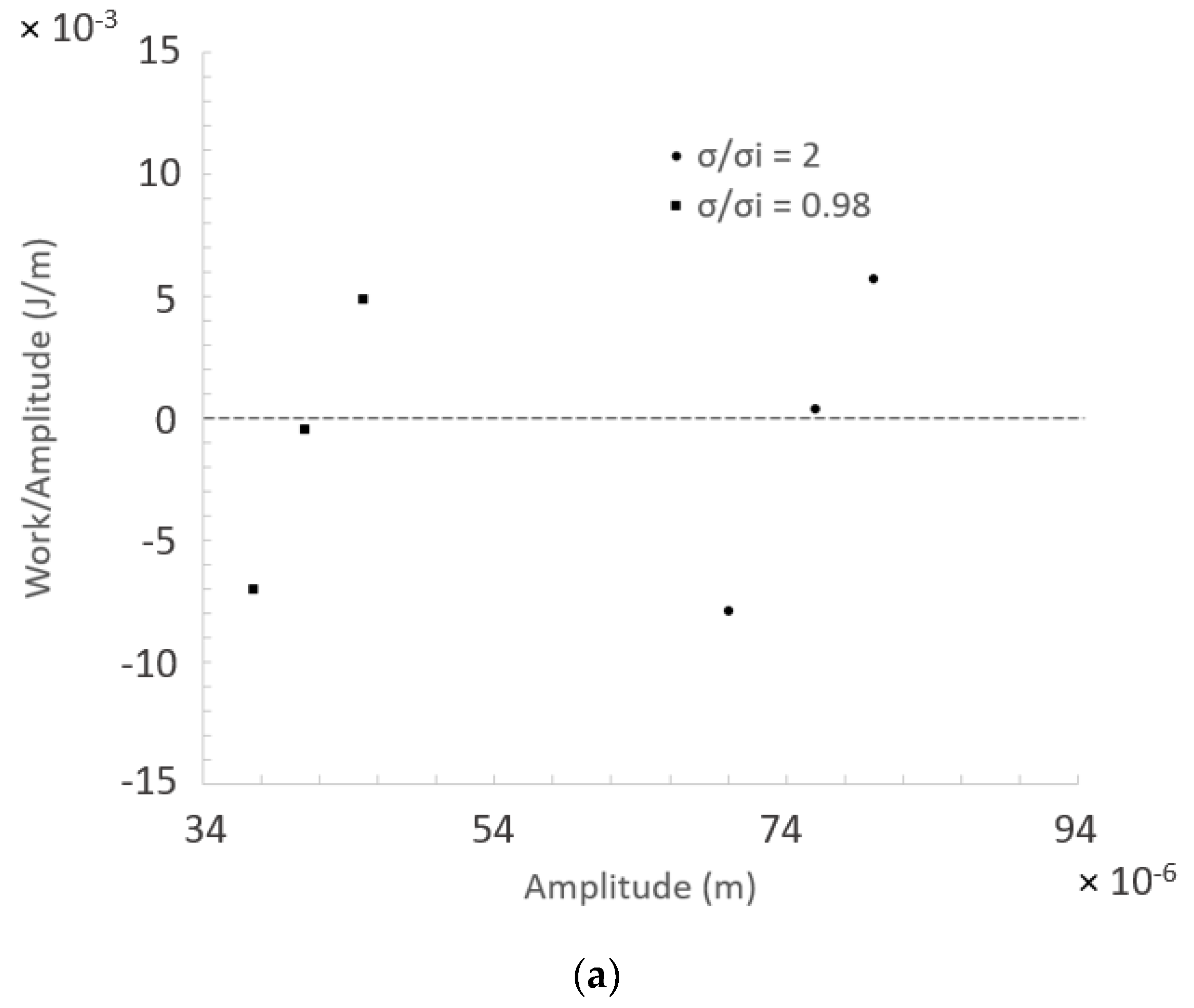
Ausoni et al. [6] measured a vibration amplitude around 0.1 mm at a distance of 80 mm in the chordwise direction and 112.5 in the spanwise direction for free-wake cavitation conditions. Since this location can be considered where the maximum vibration occurs, this value of amplitude is directly comparable with the computed q, see Equation (1). For this reason, it is assumed that for around 0.1 mm, W should be equal to zero when no wake cavitation occurs. Hence, a series of computations was carried out by changing in the CFD simulations in order to find the exact value resulting in a W null, see group (2) of Table 3. As shown in Figure 7a for free-cavitation conditions, , W = 0 was found for a value of 0.076 mm. This result shows a deviation between experiments and simulations of 24%. This discrepancy could arise from the computational domain simplifications including the 2D assumption. In particular, the predicted hydrodynamic forces might be lower in magnitude due to the fact that the domain is 2D and it does not account for the entire span length. This is supported by the fact that a similar error was also observed by Nennemann et al. [17].
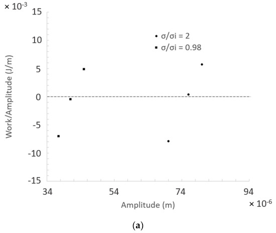

Figure 7.
Predicted maximum vibration amplitudes at the trailing edge corresponding to the points with zero work located near the dashed horizontal line (a); and displacement time histories of the first torsion mode in resonance with the von Karman vortex street for no cavitation and incipient cavitation regimes (b).
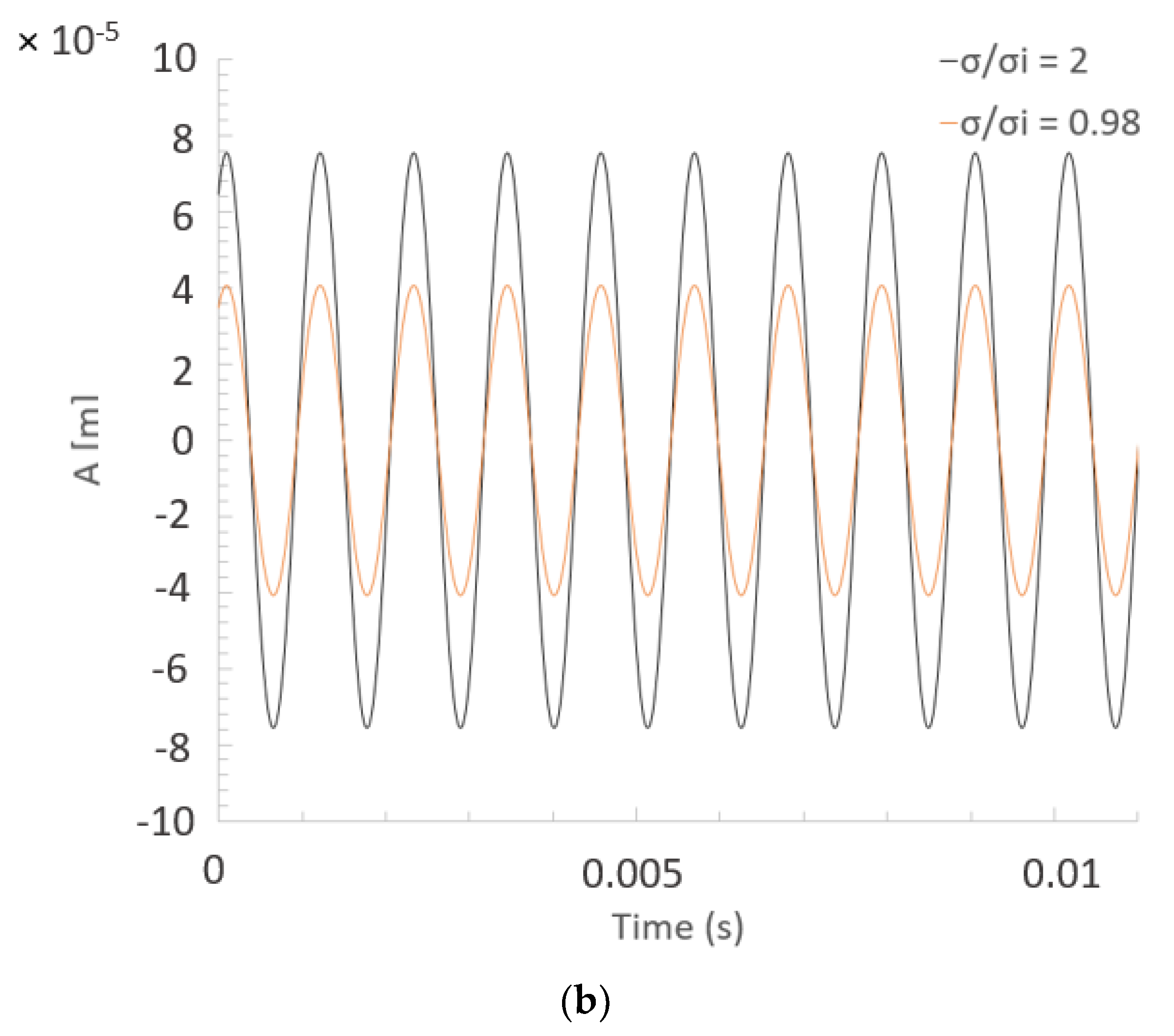
For incipient cavitation conditions, , the value of q obtained from the simulations of group (3), see Table 3, was 0.041 mm. Unfortunately, this result cannot be compared with any experimental result. Nevertheless, it shows a drop of approximately 45% in comparison with the q value corresponding to a cavitation-free condition, see Figure 7b, which is in good agreement with the drop in the vibration acceleration that was also measured by Ausoni et al. [6] when wake cavitation occurred, as shown in Figure 8.
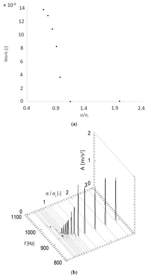
Figure 8.
Computed modal work (a) and acceleration vibration amplitude (b) measured by Ausoni et al. [6] as a function of cavitation level.
In Figure 8, the value of W computed from the simulations of group (4) is plotted as a function of the relative cavitation number when is fixed at 0.076 mm, which corresponds to the modal amplitude previously computed for a free-wake cavitation regime, see Figure 7a. In the same figure, the vibration acceleration as a function of the cavitation number derived from Ausoni et al. [6] is included for comparison.
Figure 8a shows a perfect energy balance for higher than 1 since the prescribed vibration modal amplitude, , matches q for no cavitation conditions. However, when wake cavitation appeared, the modal work began to increase, which indicates a drop in q. This trend agrees qualitatively with the drop in the vibration acceleration observed by Ausoni et al. [6].
3.3. Discussion
In this section, the streamwise velocity, the absolute pressure, the Eulerian Q criterion, and the vorticity computed in the simulations of group (4), see Table 3, are presented with the intention to show the mechanism responsible for the drop in the vibration amplitude when the cavitation number is decreased.
The plots in the figures below present results corresponding to: (i) wake-cavitation-free regime (), (ii) incipient wake cavitation regime (), and (iii) developed wake cavitation regime () at t/T = 0, corresponding to the initial hydrofoil horizontal position, and at t/T = 0.25, corresponding to the maximum displacement amplitude position, in which T is one vibration period. In Figure 9, the two corresponding hydrofoil positions and displacement directions are shown.
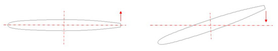
Figure 9.
Hydrofoil initial position at t/T = 0 (left) and at t/T = 0.25 when it reaches its maximum deformation (right). Red arrows indicate the displacement direction.
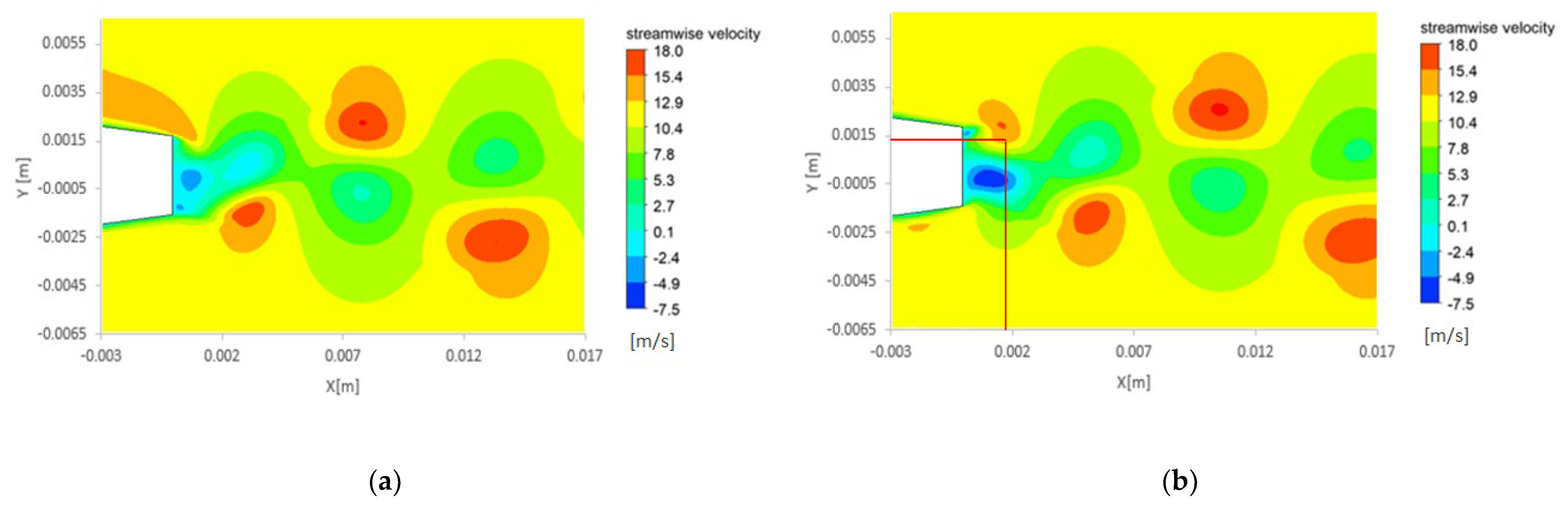
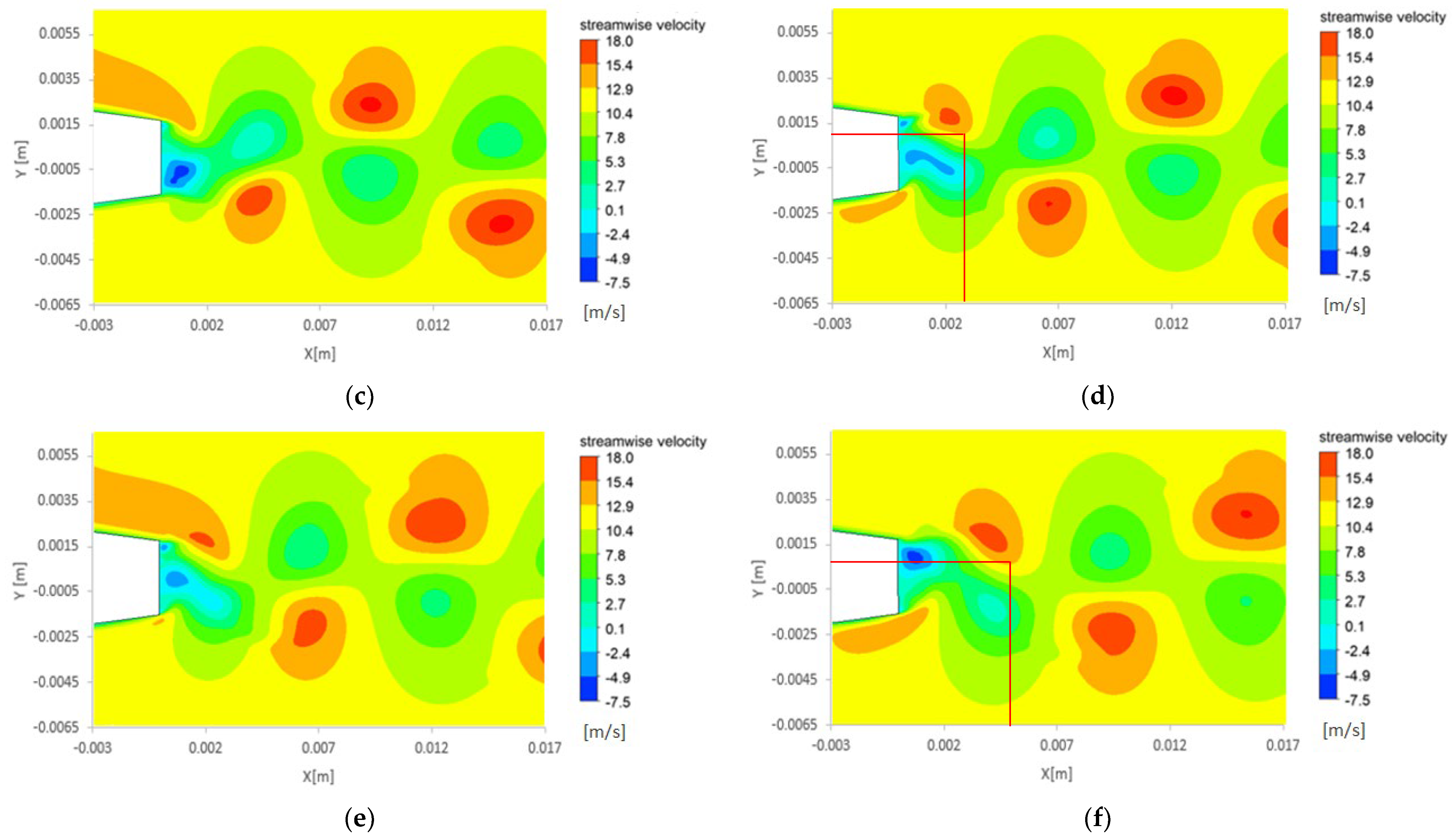
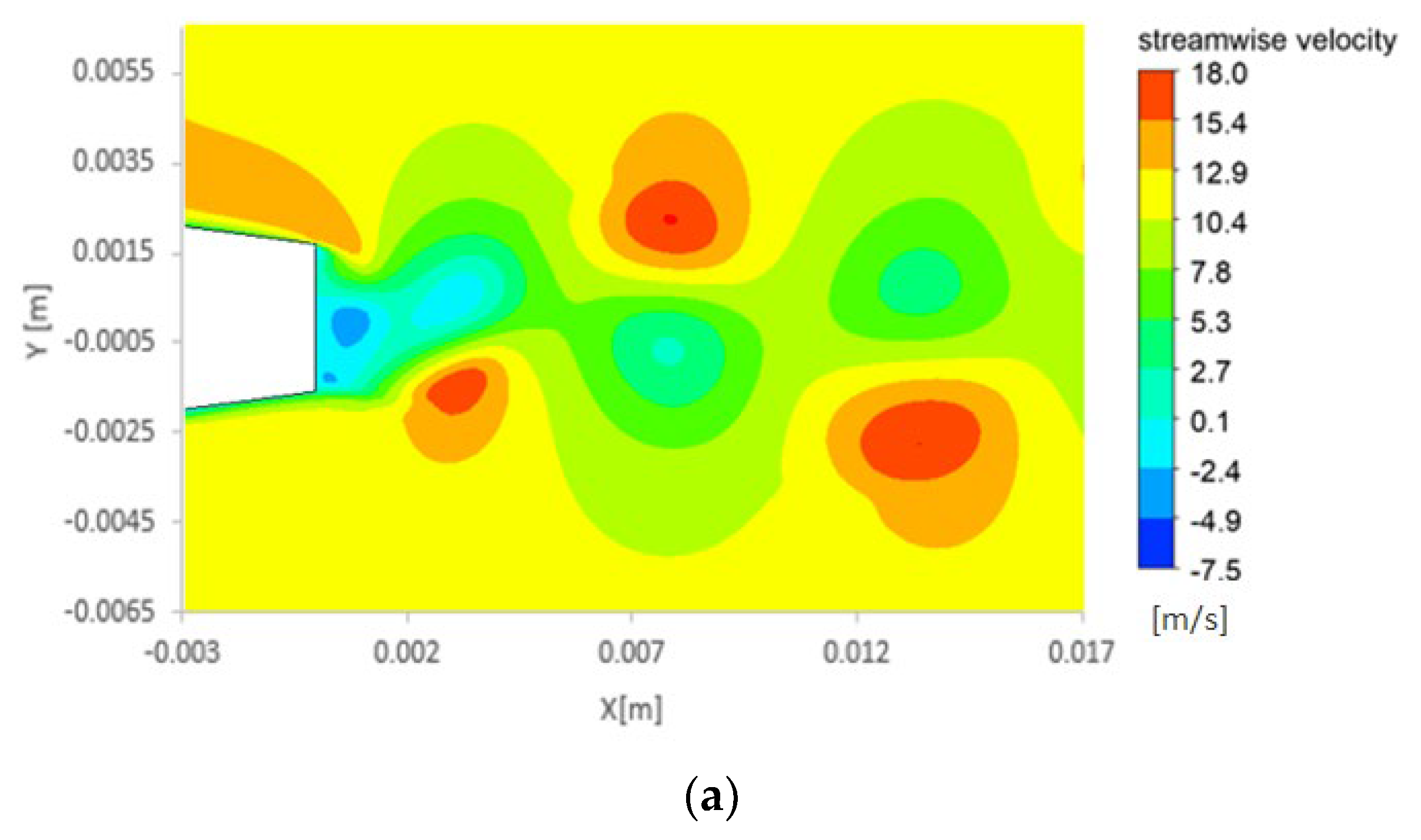
More specifically, Figure 10 shows the streamwise velocity distribution with vertical and horizontal red lines, added on the contour plots, pointing to the locations where vortices occurred. It can be observed that the vertical red line is displaced downstream when the cavitation number is reduced, indicating that the vortex shedding formation location takes place further downstream in these conditions. This phenomenon was also observed by Chen et al. [22] and Ausoni et al. [6].
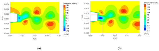
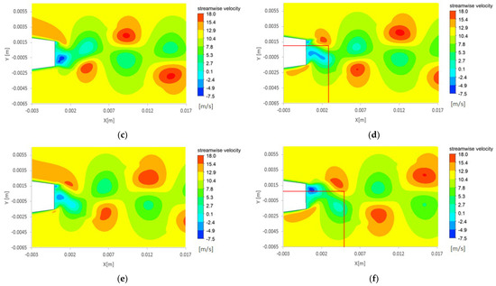
Figure 10.
Streamwise velocity for (a,b), (c,d), and (e,f) regimes at t/T = 0 (a,c,e) and t/T = 0.25 (b,d,f).
On the other hand, the horizontal red line descends along the vertical Y-axis when wake cavitation occurs, indicating a decrease of the vortex shedding formation location, which results in an increase in the vortices alignment. Again, Chen et al. [22] also observed this phenomenon numerically.
Figure 11 presents the streamwise velocity superimposed on a vapor fraction contour plot. The closed contours correspond to regions in which the vapor fraction is higher than 0.1. This figure shows how the vapor cavity acts as a sloped extension of the trailing edge and, thus, it is believed to be responsible for the displacement downstream and the descent along the Y-axis of the vortex shedding formation location, observed in Figure 10. These alterations in the velocity pattern imply changes in the force fields, which in turn influence the modal work and thus the vibration amplitude. Other authors, such as Zeng et al. [37] and Neidhardt et al. [38], also observed how sensitive the hydrofoil dynamic response is to the trailing edge geometry.

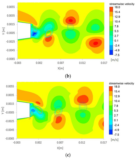
Figure 11.
Streamwise velocity superimposed on the vapor fraction (contour plot) for (a), (b), and (c) regimes at t/T = 0 (a,b,c).
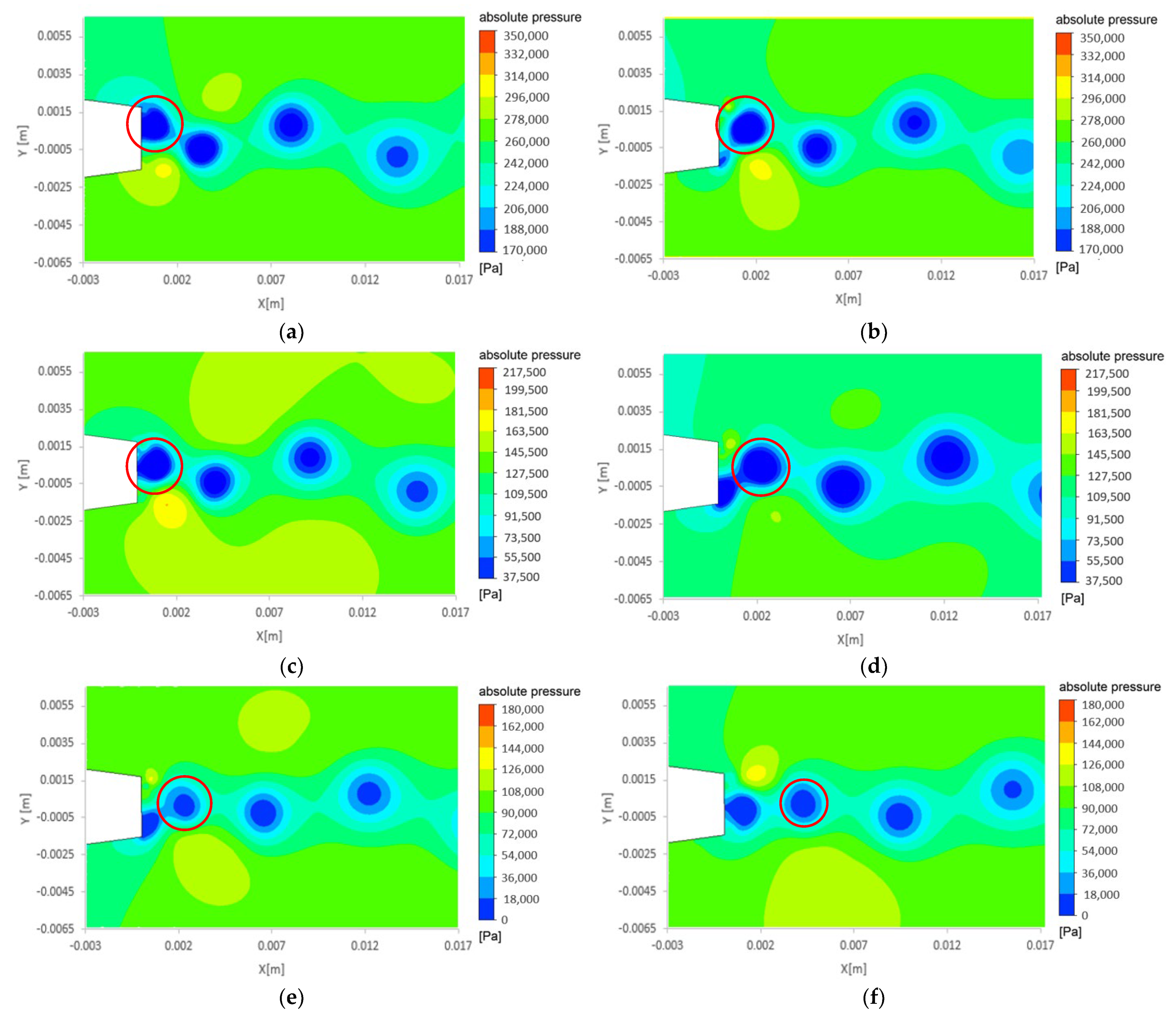
Figure 12 shows the absolute pressure pattern. The pressure scales were adjusted in the range ± 90,000 Pa around the outlet absolute pressure in order to improve the comparison. The pressure drops corresponding to equivalent vortices between regimes are highlighted in red.
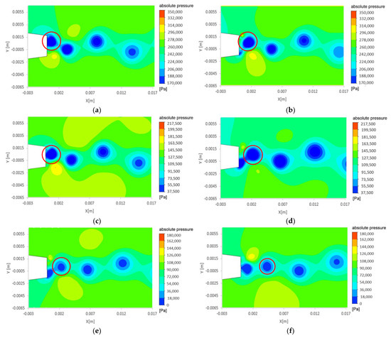
Figure 12.
Absolute pressure for (a,b), (c,d), and (e,f) regimes at t/T = 0 (a,c,e) and t/T = 0.25 (b,d,f).
In addition to the displacement of the vortex shedding formation location observed previously, a pressure drop at the bottom of the trailing edge for the developed wake cavitation regimes can be seen at t/T = 0.
This pressure drop at the bottom of the trailing edge is responsible for a positive pressure gradient in the direction of the trailing edge displacement. For this reason, it is believed to be the cause of the increase in the modal work over a vibration period and thus of the decrease in the vibration amplitude.
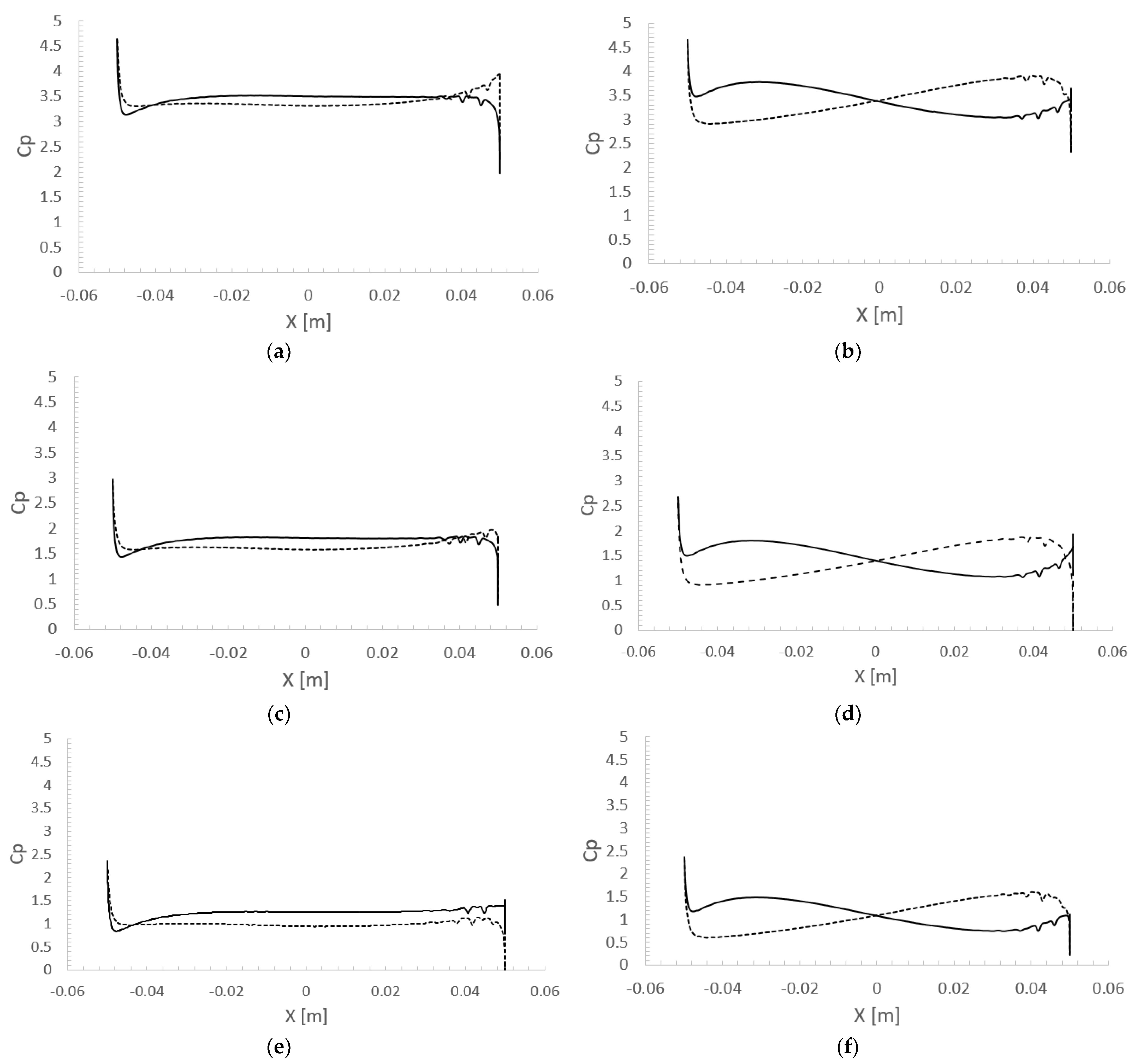
Figure 13 presents the plots of the pressure coefficient, , over the NACA 0009 profile at different instants. The dashed line corresponds to the lower side of the hydrofoil and the solid one to the upper side.
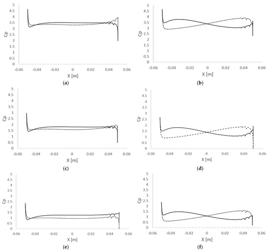
Figure 13.
Cp coefficient over the NACA 0009 profile for (a,b), (c,d), and (e,f) regimes at t/T = 0 (a,c,e) and t/T = 0.25 (b,d,f).
Whereas the graphs at t/T = 0.25 look very similar, at t/T = 0 and around the trailing edge at location X = 0.055 m, significant differences can be observed. For instance, the pressure at the bottom of the trailing edge was higher than the one at the top of the trailing edge for a free-wake cavitation condition. Nevertheless, this pressure pattern was reversed when wake cavitation occurred. For conditions, the pressure at the bottom of the trailing edge was lower than the one at the top of the trailing edge. As previously mentioned, this pressure pattern resulted in a positive pressure gradient in the direction of the hydrofoil displacement and thus in an increase in the modal work.
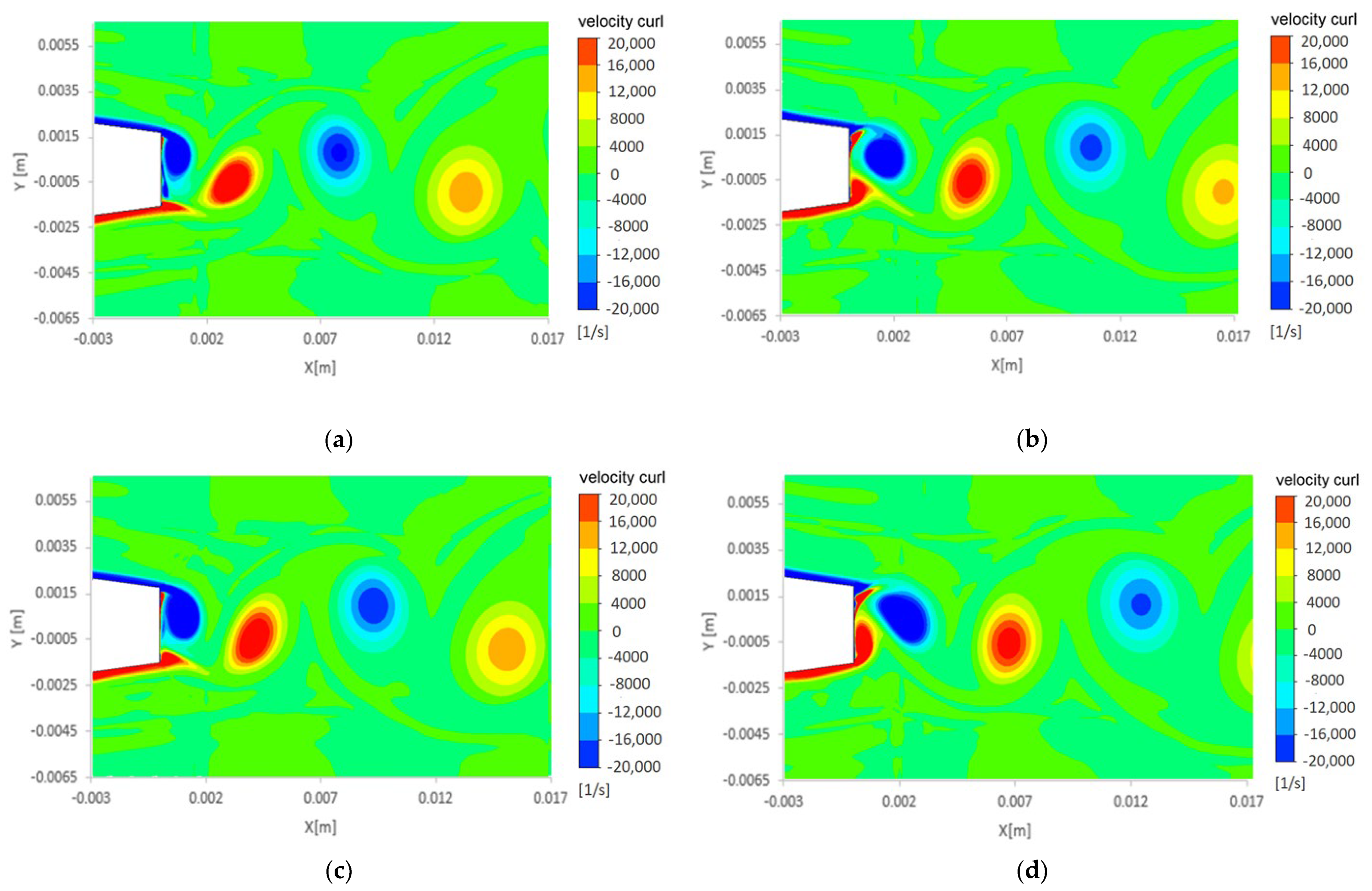
In addition to pressure forces, viscous forces are also relevant in this canonical flow pattern since they play a key role in determining the value of the Eulerian Q criterion, see Figure 14, and the velocity curl, see Figure 15. Both figures show that at instant t/T = 0.25 when the maximum deformation at the trailing edge occurred, the top vortex was closer to the trailing edge without cavitation; meanwhile, it is located further downstream for cavitation conditions, see the vortex highlighted in green in Figure 14. As a result, the larger area left just behind the trailing edge in cavitation conditions was occupied by a new vortex at the bottom row. This vortex resulted in a pressure drop at this location while the trailing edge wall was ascending. As previously observed, this pressure drop led to a positive pressure gradient in the direction of the trailing edge displacement, which is considered to be responsible for the increase in the modal work and thus for the decrease in the vibration amplitude.
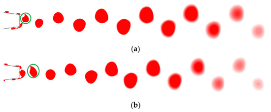
Figure 14.
Contour plots of the Eulerian Q criterion in the range from 1,000,000 to 3,000,000 s−2 for no cavitation, (a), and cavitation, (b), regimes at t/T = 0.25.
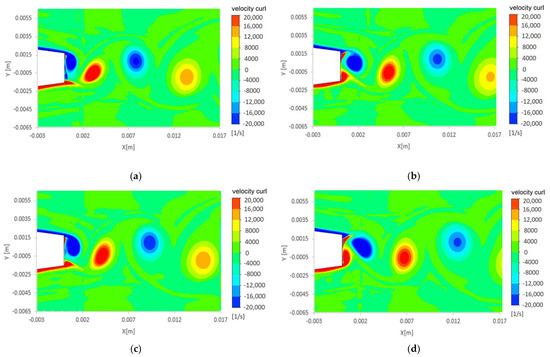
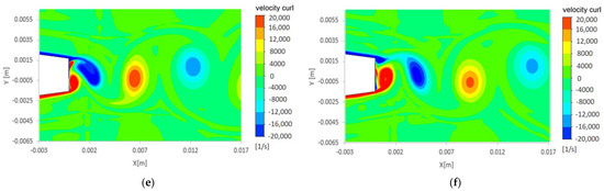
Figure 15.
Velocity curl for (a,b), (c,d), and (e,f) regimes at t/T = 0 (a,c,e) and t/T = 0.25 (b,d,f).
Figure 15 also shows that the magnitude of the velocity curl was similar in value for different cavitation regimes. This observation leads us to conclude that the wake cavitation has a negligible influence on the velocity curl magnitude. Therefore, the increase in the modal work should be mainly induced by the pressure forces instead of the viscous ones. However, on the other hand, the wake cavitation clearly modified the vorticity geometry. It can be seen that the vortices were stretched in the streamwise direction for cavitation conditions. This phenomenon was also observed numerically by Chen et al. [22].
4. Conclusions
In this paper, essentially two studies were presented: (i) the computation of the vibration amplitude of a NACA 0009 hydrofoil under a torsional lock-in condition for cavitation and non-cavitation flow conditions and (ii) the study of the wake cavitation influence on the modal work, i.e., on the vibration amplitude of the hydrofoil under a torsional lock-in condition.
Regarding the prediction of the vibration amplitudes, the following conclusions can be drawn:
- The modal work approach can be employed to compute the vibration amplitude of a hydrofoil under a torsional lock-in condition for both cavitation-free and incipient cavitation conditions.
- The drop in the vibration amplitude when wake cavitation occurs is around 45%.
- The deviation in the numerically simulated vibration amplitude relative to the experimental results is approximately 24% for a cavitation-free condition.
Whereas concerning the influence of the wake cavitation on the vibration amplitude:
- The von Karman vortex cavitation seems to create an additional extension of the trailing edge solid boundary, which results in a significant alteration of the near-wake flow dynamics.
- When wake cavitation occurs, the vortex formation location is displaced downstream, which results in an additional space between the vortex and the trailing edge. This additional space allows an early occurrence of an opposite vortex and hence a drop in pressure at this location.
- The increase in the modal work, which corresponds to a decrease in the vibration amplitude, seems not to be as dependent on viscous forces as it is on pressure ones. Specifically, the early occurrence of the vortex is believed to be responsible for a positive pressure gradient in the trailing edge wall displacement direction and thus for the increment of the modal work.
These results improve the understanding of the FSI interaction phenomenon that determine the dynamic loads exerted by the cavitating von Karman vortex shedding on a hydrofoil, which can be used to detect and prevent undesired resonance conditions prone to occur in hydraulic turbines working at off-design conditions.
Author Contributions
Conceptualization, R.R., O.d.l.T. and X.E.; methodology, R.R. and J.C.; numerical simulations, R.R. and J.C.; investigation, R.R, O.d.l.T. and X.E.; writing—original draft preparation, R.R.; writing—review and editing, R.R., O.d.l.T. and X.E.; supervision, O.d.l.T. and X.E.; funding acquisition, X.E. All authors have read and agreed to the published version of the manuscript.
Funding
This research was funded by Horizon 2020 research and innovation program under grant agreement No 814958.
Conflicts of Interest
The authors declare no conflict of interest.
References
- Strouhal, V. Uber eine besondere Art der Tonerregung. Ann. Phys. Chem. 1878, 10, 216–251. [Google Scholar] [CrossRef] [Green Version]
- Von Kármán, T. Ueber den Mechanismus des Widerstandes, den ein bewegter Körper in einer Flüssigkeit erfährt. Nachrichten von der Gesellschaft der Wissenschaften zu Göttingen Mathematisch-Physikalische Klasse 1911, 1911, 509–517. [Google Scholar]
- Von Kármán, T. Ueber den Mechanismus des Widerstandes, den ein bewegter Körper in einer Flüssigkeit erfährt. Nachrichten von der Gesellschaft der Wissenschaften zu Göttingen Mathematisch-Physikalische Klasse 1912, 1912, 547–556. [Google Scholar]
- Gerrard, J.H. The mechanics of the formation region of vortices behind bluff bodies. J. Fluid Mech. 1966, 25, 401–413. [Google Scholar] [CrossRef]
- Perry, A.E.; Chong, M.S.; Lim, T.T. The vortex-shedding process behind two-dimensional bluff-bodies. J. Fluid Mech. 1982, 116, 77–90. [Google Scholar] [CrossRef]
- Ausoni, P. Turbulent Vortex Shedding from a Blunt Trailing Edge Hydrofoil. Ph.D. Thesis, EPFL, Lausanne, Switzerland, 2009. [Google Scholar]
- Naudascher, E.; Rockwell, D. Flow Induced Vibrations: An Engineering Guide; Dover Publications Inc.: Mineola, NY, USA, 2005. [Google Scholar]
- Blevins, R. Flow-Induced Vibrations; Krieger Publishing Company: Malabar, FL, USA, 2001. [Google Scholar]
- Arioli, G.; Gazzola, F. Torsional instability in suspension bridges: The tacoma narrows bridge case. Commun. Nonlinear Sci. Numer. Simul. 2017, 42, 342–357. [Google Scholar] [CrossRef] [Green Version]
- Hoskoti, L.; Misra, A.; Sucheendran, M.M. Frequency lock-in during vortex induced vibration of a rotating blade. J. Fluids Struct. 2018, 80, 145–164. [Google Scholar] [CrossRef]
- Gummer, J.H.; Hensman, P.C. A review of stay vane cracking in hydraulic turbines. Int. Water Power Dam Constr. 1992, 44, 32–42. [Google Scholar]
- Lockey, K. Flow induced vibrations at stay vanes: Experience at site and CFD simulation of von Kármán vortex shedding. In Proceedings of the Hydro 2006, Porto Carras, Greece, 25 September 2006; pp. 25–28. [Google Scholar]
- Dörfler, P.; Sick, M.; Coutu, A. Flow Induced Pulsation and Vibration in Hydroelectric Machinery; Springer Science & Business Media: London, UK, 2013. [Google Scholar] [CrossRef]
- Pang, L.J.; Lu, G.P.; Zhong, S.; Liu, J.S. Vortex shedding simulation and vibration analysis of stay vanes of hydraulic turbine. J. Mech. Eng. 2011, 47, 159–166. [Google Scholar] [CrossRef]
- Vu, T.C.; Nennemann, B.; Ausoni, P.; Farhat, M.; Avellan, F. Unsteady CFD prediction of von Karman vortex shedding in hydraulic turbine stay vanes. In Proceedings of the Hydro 2007, Granada, Spain, 15–17 October 2007. [Google Scholar]
- Alexandre, A.N.; Gissoni, H.; Gonçalves, M.; Cardoso, R.; Jung, A.; Meneghini, J. Engineering diagnostics for vortex-induced stay vanes cracks in a Francis turbine. IOP Conf. Ser. Earth Environ. Sci. 2016, 49, 072017. [Google Scholar]
- Nennemann, B.; Monette, C. Prediction of vibration amplitudes on hydraulic profiles under von Karman vortex excitation. Conf. Ser. Earth Environ. Sci. 2019, 240, 062004. [Google Scholar] [CrossRef]
- Arndt, R.E. Cavitation in fluid machinery and hydraulic structures. Annu. Rev. Fluid Mech. 1981, 13, 273–326. [Google Scholar] [CrossRef]
- Franc, J.P.; Michel, J.M. Fundamentals of Cavitation; Springer Science & Business Media: Berlin, Germany, 2006; pp. 1–13, 247–262. [Google Scholar]
- Young, J.O.; Holl, J.W. Effects of cavitation on periodic wakes behind symmetric wedges. J. Fluids Eng. 1966, 88, 163–176. [Google Scholar] [CrossRef]
- Belahadji, B.; Franc, J.P.; Michel, J.M. Cavitation in the rotational structures of a turbulent wake. J. Fluid Mech. 1995, 287, 383–403. [Google Scholar] [CrossRef]
- Chen, J.; Geng, L.; Excaler, X. Numerical investigation of the cavitation effects on the vortex shedding from a Hydrofoil with blunt trailing edge. Fluids 2020, 5, 218. [Google Scholar] [CrossRef]
- Ramamurthy, A.S.; Balachandar, R. Characteristics of constrained cavitating bluff body wakes. J. Eng. Mech. 1991, 117, 513–531. [Google Scholar] [CrossRef]
- Zeng, Y.; Yao, Z.; Gao, J.; Hong, Y.; Wang, F.; Zhang, F. Numerical investigation of added mass and hydrodynamic damping on a blunt trailing edge hydrofoil. J. Fluids Eng. 2019, 141, 081108. [Google Scholar] [CrossRef]
- Liaghat, T.; Guibault, F.; Allenbach, L.; Nennemann, B. Two-Way Fluid-Structure Coupling in Vibration and Damping Analysis of an Oscillating Hydrofoil. ASME 2014, 46476, V04AT04A073, Paper No. IMECE2014-38441. [Google Scholar]
- Zeng, Y.S.; Yao, Z.F.; Yang, Z.J.; Wang, F.J.; Hong, Y.P. The Prediction of Hydrodynamic Damping Characteristics of a Hydrofoil With Blunt Trailing Edge. IOP Conf. Ser. Earth Environ. Sci. 2017, 163, 012041. [Google Scholar] [CrossRef]
- Alexandre, A.N.; Saltara, F. Study of Stay Vanes Vortex-Induced Vibrations with different Trailing-Edge Profiles Using CFD. J. Fluid Mach. Syst. 2009, 2, 4. [Google Scholar]
- Miyagawa, K.; Fukao, S.; Kawata, Y. Study on stay vane instability due to Vortex shedding. In Proceedings of the 22th IAHR Symposium on Hydraulic Machinery and Systems, Stockholsm, Sweden, 29 June–2 July 2004. [Google Scholar]
- Williamson, C.H. Vortex dynamics in the cylinder wake. Annu. Rev. Fluid Mech. 1996, 28, 477–539. [Google Scholar] [CrossRef]
- Kim, J.; Choi, H. Distributed forcing of flow over a circular cylinder. Phys. Fluids 2005, 17, 103–116. [Google Scholar] [CrossRef]
- Roshko, A. On the Drag and Shedding Frequency of Two-Dimensional Bluff Bodies; National Aeronautics and Space Administration: Washington, DC, USA, 1954. [Google Scholar]
- Farhadi, M.; Sedighi, K.; Korayem, A.M. Effect of wall proximity on forced convection in a plane channel with a built-in triangular cylinder. Int. J. Therm. Sci. 2010, 49, 1010–1018. [Google Scholar] [CrossRef]
- Liang, Q.W.; Rodriguez, C.G.; Egusquiza, E.; Escaler, X.; Farhat, M.; Avellan, F. Numerical simulation of fluid added mass effect on a Francis turbine runner. Comput. Fluids 2007, 36, 1106–1118. [Google Scholar] [CrossRef]
- Escaler, X.; De La Torre, O. Axisymmetric vibrations of a circular Chladni plate in air and fully submerged in water. J. Fluids Struct. 2018, 82, 432–445. [Google Scholar] [CrossRef]
- Zhu, W.R.; Gao, Z.X.; Lu, L.; Wang, F.J. Analysis and Optimization on Natural Frequencies Depreciation Coefficient of Centrifugal Pump Impeller in Water. J. Hydraul. Eng. 2013, 44, 1455–1461. [Google Scholar]
- Celik, I.B.; Ghia, U.; Roache, P.J.; Freitas, C.J.; Coleman, H.; Raad, P.E. Procedure for Estimation and Reporting of Uncertainty Due to Discretization in CFD Applications. J. Fluids Eng. 2008, 130, 078001. [Google Scholar] [CrossRef] [Green Version]
- Zeng, Y.S.; Yao, Z.F.; Zhou, P.J.; Wang, F.J.; Hong, Y.P. Numerical investigation into the effect of the trailing edge shape on the added mass and hydrodynamic damping for a hydrofoil. J. Fluids Struct. 2019, 88, 167–184. [Google Scholar] [CrossRef]
- Neidhardt, T.; Jung, A.; Heyneck, S.; Gummer, J. An alternative approach to the von Karman vortex problem in hydraulic turbines. In Proceedings of the Hydro 2017, Seville, Spain, 2 November 2017. [Google Scholar]


Publisher’s Note: MDPI stays neutral with regard to jurisdictional claims in published maps and institutional affiliations. |
© 2021 by the authors. Licensee MDPI, Basel, Switzerland. This article is an open access article distributed under the terms and conditions of the Creative Commons Attribution (CC BY) license (https://creativecommons.org/licenses/by/4.0/).