
Nonlinear Causality between Crude Oil Prices and Exchange Rates: Evidence and Forecasting


Department of Applied Informatics and Mathematics in Economics, Faculty of Economic Sciences and Management, Nicolaus Copernicus University in Torun, ul. Gagarina 13a, 87-100 Torun, Poland
Energies 2021, 14(19), 6043; https://doi.org/10.3390/en14196043
Submission received: 19 August 2021
/
Revised: 14 September 2021
/
Accepted: 20 September 2021
/
Published: 23 September 2021
(This article belongs to the Special Issue Transformation of Energy Markets: Description, Modeling of Functioning Mechanisms and Determining Development Trends)
Abstract
:The relationships between crude oil prices and exchange rates have always been of interest to academics and policy analysts. There are theoretical transmission channels that justify such links; however, the empirical evidence is not clear. Most of the studies on causal relationships in this area have been restricted to a linear framework, which can omit important properties of the investigated dependencies that could be exploited for forecasting purposes. Based on the nonlinear Granger causality tests, we found strong bidirectional causal relations between crude oil prices and two currency pairs: EUR/USD, GBP/USD, and weaker between crude oil prices and JPY/USD. We showed that the significance of these relations has changed in recent years. We also made an attempt to find an effective strategy to forecast crude oil prices using the investigated exchange rates as regressors and vice versa. To this aim, we applied Support Vector Regression (SVR)—the machine learning method of time series modeling and forecasting.
1. Introduction
The crucial role of crude oil in the world economy has implied a discussion on links between oil prices and other macroeconomic and financial variables. Both theoretical and empirical research have pointed out some sources and potential consequences of these links (cf. [1]). It has been noticed that one of the most important factors connected with crude oil prices is exchange rates. The relation between oil prices and exchange rates has always been of interest to academics and policy analysts. Theory indicates various mechanisms which explain this relationship. They refer not only to direct ways how both variables affect each other but also to indirect transmission channels referring to specific macroeconomic or financial factors [2]. It should be noted that both directions of causation are well-founded. On the one hand, crude oil prices affect exchange rates. Crude oil is the most important source of energy in the world, and its price does not offer a substantial arbitrage opportunities. On the other hand, exchange rate connects the internal and external economies, hence in market-oriented and open economies crude oil prices exert on exchange rates [3]. More specifically, three direct transmission channels of oil prices to exchange rates can be indicated: the terms of the trade channel, the wealth effect channel, and the portfolio reallocation channel [4]. On the other hand, reverse causality from exchange rates to crude oil prices is also theoretically motivated. The main reason for this fact is that oil prices are denominated in USD. An appreciation of the U.S. dollar increases the price of oil in domestic currencies for countries besides the U.S., which directly affects the oil supply and demand. Moreover, exchange rates can also affect oil prices directly through financial markets or indirectly via other financial assets, and through portfolio rebalancing and hedging practices in particular [5].
The relationships between crude oil prices and exchange rates have been the topic of a rapidly growing body of empirical literature over the past two decades (cf. [1,3,6,7,8,9]). The general literature on this issue can be divided into four main research areas: links between exchange rates and imported crude oil prices, causality analysis, variance decomposition and impulse response, and the influence of crisis [7]. The obtained results showed that the relations between crude oil prices and exchange rates can differ in time length. Many studies found long-run connections between oil prices and exchange rates. There is also much weaker evidence for short-run linkages and spillovers between both variables at daily and monthly frequencies (cf. [1,3]). Moreover, it has been shown that the detected relationships are time-varying, which can be the effect of their nonlinear or asymmetric mechanism [3].
The main purpose of our paper was to test for bidirectional Granger causality between crude oil prices and selected exchange rates, namely, EUR/USD, GBP/USD, and JPY/USD, and to analyze its stability. In econometrics, Granger causality is one of the most popular concepts of causality. It provides not only a strong insight into the mechanism of the relationships, but most of all indicates the potential ability to predict investigated time series. In the economic literature, Granger causality is usually tested in the framework of linear dependencies, represented by VAR models (cf. [10]). In particular, linear Granger causality between crude oil prices and exchange rates has been studied by [2,7,9,11,12,13,14,15,16]. The obtained results are not so clear on the direction of the causal relationship between these two variables; however, some authors found evidence for bidirectional causality (see [1,9]). On the other hand, it has been generally noted that the linear approach is not sufficient in the case of nonlinear relations (e.g., [17,18,19]). Many studies have confirmed the nonlinear dynamics of financial and economic systems, which indicates the need for including nonlinear causality tests in studies. Otherwise, one can omit important properties of the investigated dependencies that could be exploited for forecasting purposes (cf. [10]). The nonlinear analysis of the relationships between crude oil prices and exchange rates has been performed much more rarely than the linear one, but the obtained results show that it can give a better insight into the mechanism of the investigated dependencies (e.g., [8,20,21,22,23,24]). It has been argued that the nonlinear causality behavior between oil prices and exchange rates can be explained by asymmetric responses of economic activity to oil price shocks [25,26,27], the negative effects of oil price uncertainty on economic activity [28], structural breaks, persistence and discontinuity in the adjustment (cf. [21]).
For these reasons, in our study, we tested for nonlinear causality, using two nonlinear causality tests, introduced by Hiemstra and Jones [18] and Diks and Panchenko [29]. Moreover, we divided the analyzed period into two subperiods in order to verify if the existing causalities were stable over time.
It has been concluded in the literature that the frequent finding that exchange rates and oil prices move together (especially over the long-run) does not necessarily imply that one is useful when forecasting the other. The reason is that past relationships do not necessarily hold in the future and the link between in-sample and out-of-sample is often rather weak [1]. That is why the purpose of our study was not limited only to detecting causality between the investigated series, but additionally to make an attempt to exploit these relations for effective forecasting. As the predictor, we applied Support Vector Regression (SVR)—the machine learning method of time series modeling and forecasting. In recent years, specific machine learning techniques have been successfully applied for forecasting purposes. They are data-driven, self-adaptive methods requiring very few assumptions concerning the investigated data. The support vector regression model [30] is based on the support vector machine method [31], which was originally introduced to solve classification problems. It is designed to have a good power of generalization and an overall stable behavior, which implies a good out-of-sample performance. Many studies in the literature have shown that SVR models can give more accurate forecasts than alternative machine learning methods and can be successfully used to forecast financial time series, such as stock indices, stock prices, future contracts, or exchange rates (see, e.g., [32,33,34,35]). SVR and SVR-based models have also been applied to forecast crude oil prices [36,37,38,39,40,41] or exchange rates [42,43,44,45,46]. However, it should be noted that most of these models were autoregressive. In particular, to the best of our knowledge, there has not been an attempt to incorporate crude oil prices and exchange rates jointly to the SVR model, using one of these variables as the regressor for the second one. In our study, we construct and analyzed such SVR models to verify if potential predictability (ensured by the existence of Granger causality) really can result in more accurate forecasts.
The paper has three main contributions:
- First, we found strong nonlinear causal relationships between crude oil prices and most investigated exchange rates;
- Second, we showed that the significance of the detected relationships has changed in recent years;
- Third, we applied SVR models of different kernels and regressors to verify if it is possible to exploit the detected relationships for effective forecasting.
2. Materials and Methods
2.1. Data
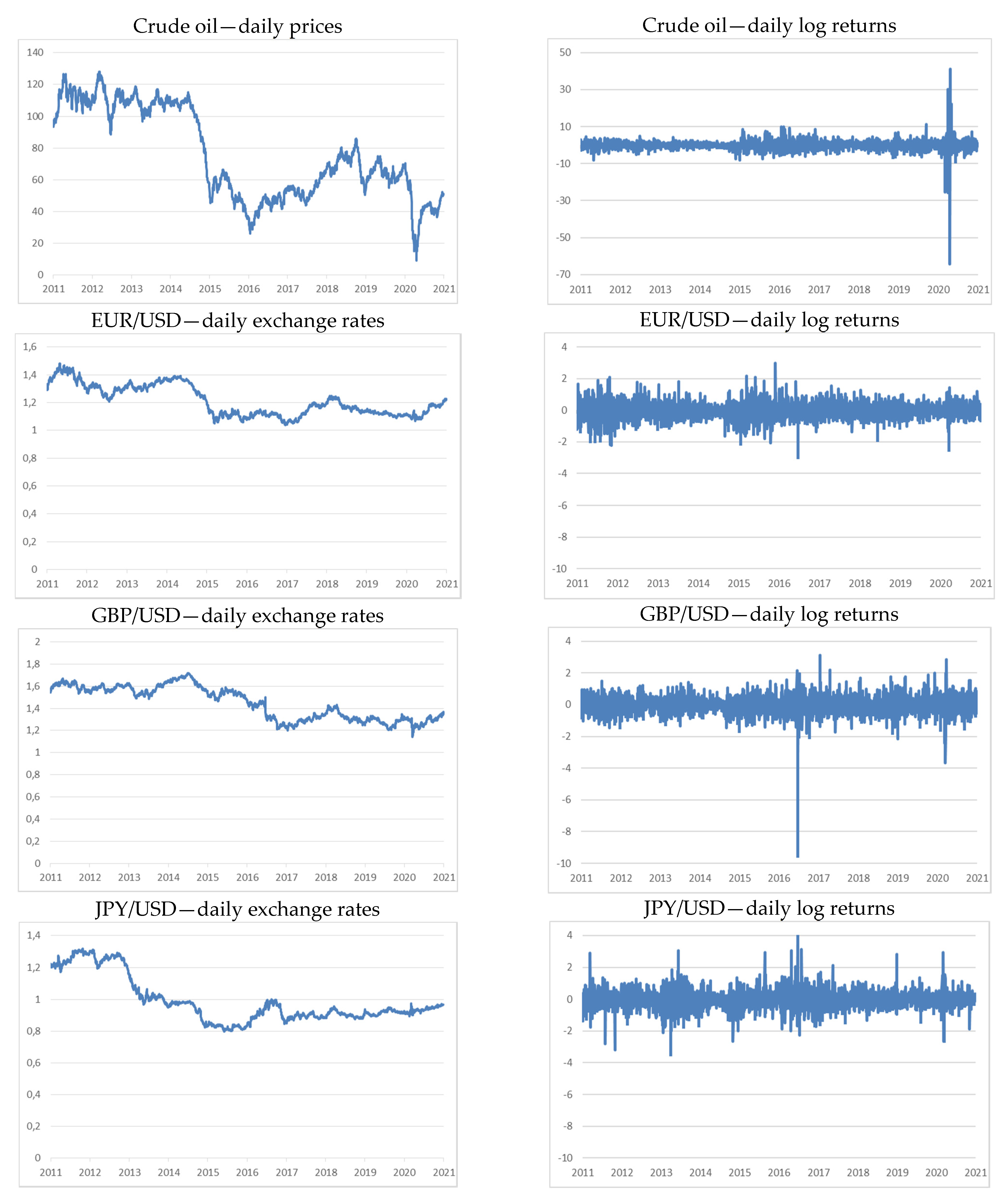
Our dataset consisted of the Brent spot prices’ FOB (published by the United States Energy Information Administration (EIA)) and the exchange rates of three most heavily traded currency pairs in the forex market, namely EUR/USD, GBP/USD, and JPY/USD. We analyzed the daily data from 3 January 2011 to 31 December 2020. However, in order to verify if the existing causalities were stable over time, we divided the analyzed period into two separate subperiods. For comparison purposes (i.e., to preserve the same power of the applied tests), we considered two subperiods of the same length—from 3 January 2011 to 31 December 2015 (Period 1) and from 4 January 2016 to 31 December 2020 (Period 2). All data were transformed to log returns using the formula , where is the price at time . The investigated time series are presented in Figure 1. One can see differences between both subperiods under study. There was a strong decline in crude oil prices at the end of Period 1, which was the effect of the decisions of the U.S. and OPEC countries to increase production, resulting in oversupply of crude oil compared to demand. The crude oil prices were stabilized at clearly lower levels in Period 2. On the other hand, the plot for daily log returns showed that the volatility of crude oil prices increased in Period 2. This conclusion is confirmed by the descriptive statistics in Table 1.
For all investigated series, the calculated means were negative in the whole period and in Period 1. Other statistics showed noticeable differences between crude oil and exchange rates; crude oil proved to be much more volatile than the exchange rates (especially in Period 2). As a consequence, it was characterized by the highest absolute values of the minimum and maximum returns and a very high standard deviation. Moreover, the distribution of crude oil returns exhibited the strongest skewness (except Period 1) and the highest kurtosis. According to the results of the Ljung–Box test, only the returns for crude oil were autocorrelated.
2.2. Nonlinear Causality Tests
The most general definition of Granger causality is formulated in terms of conditional probability distributions [47]. It states that does not Granger-cause if:
where is a strictly stationary bivariate stochastic process and denotes the conditional cumulative distribution function. According to the definition, when Equation (1) is not satisfied, we say that is a Granger cause of (denoted: XY).
In causality testing, it is assumed that the lags of the processes and are finite; hence, the null hypothesis of noncausality is expressed by the formula:
for given , . It is convenient to reformulate Condition (2) using the lagged vectors of and , i.e., and . In this notation, it takes the form:
Due to its generality, Equation (3) is not easy to verify in practice. Therefore, it is often reduced to the equality of the means of both conditional distributions and considered in the linear framework using VAR models. However, this approach has low power against many nonlinear alternatives. For this reason, Baek and Brock [17] introduced the alternative definition and the test for nonlinear Granger causality, using the correlation integrals. Formally, for a multivariate random vector , the associated correlation integral is the probability of finding two independent realizations of the vector at a distance smaller than (or equal to) , i.e.,
where are independent copies of , is the supremum norm, and denotes the indicator function that equals 1 when and are within the supremum-norm distance of each other, and 0 otherwise. In the concept of Baek and Brock, does not nonlinearly Granger-cause if:
Equation (5) states that the conditional probability that and are within the distance given that the corresponding lagged vectors and are -close, remains the same as when, in addition, one also conditions on the vectors and being -close. This means that lags of do not incrementally help to predict the next period’s value of , given lags of .
Note that based on the definition of the conditional probability, the null hypothesis of Granger nonlinear noncausality given by (5) may be expressed as follows:
where C1, C2, C3, and C4 are the correlation integrals of the form:
Given time series and of realizations on and , Equation (6) is verified using the estimators of the correlation integrals (7)–(10):
where , .
Hiemstra and Jones [18] modified the test introduced by Baek and Brock by relaxing its assumptions. According to their testing procedure (H-J test), for the given values of , , and , under the assumptions that and are strictly stationary, weakly dependent, and satisfy the mixing conditions of Denker and Keller [48], if does not strictly Granger-cause then:
where the definition and the estimator of were given in the Appendix of Hiemstra and Jones [18].
It was noted by Diks and Panchenko [49] that the H-J test is not fully compatible with the definition of Granger causality; hence, it may lead to over-rejection of the null hypothesis of noncausality. Therefore, they proposed an alternative test (D-P test) which overcomes these inadequacies [29]. Their test statistics takes the form:
where and . In the case of , Diks and Panchenko proved that their test statistics is asymptotically distributed as standard normal and diverges to positive infinity.
It should be noted that the value of the test statistics in both the H-J and D-P tests depends on the parameters , and . In practice, lags are considered, where is a fixed natural number. In the studies presented in the literature, the value of a distance measure between 0.5 and 1.5 is recommended for consideration (cf. [18,29,50]).
2.3. Support Vector Regression
Consider the regression model:
where is the unknown regression function, is the dependent variable, is the vector of explanatory variables, and is an additive zero-mean noise with variance . The general purpose of SVR is to use a training dataset to approximate by a function , which has, at most, deviation from the outputs and is as flat as possible [51]. To construct the SVR function , the vectors are mapped onto a high-dimensional space using some specific nonlinear transformation, and next, the coefficients of the linear model:
are estimated, where is the space dimension, are the transformation functions, denote the model coefficients, and is the bias term [52,53]. In order to estimate and , the -insensitive loss function:
has been proposed [31]. By its construction, does not penalize errors below some , chosen a priori. This means that training points within the ε-margin have no loss; hence, only points located outside the ε-margin are used as the support vectors to estimate the model. However, the accuracy of the approximation (measured by the function ) is not the only postulate taken into account in SVR. Besides it, SVR tries to reduce the model complexity by minimizing the formula , where . In many cases, it is not possible to approximate all observations in the training set with an error below (cf. [54]). Therefore, in order to allow for greater errors, one incorporates nonnegative slack variables and , which represent the upper and lower constraints, s.t.:
for all . Finally, the function is indicated as the minimum of the functional:
where is some prespecified positive value (cf. [55]). The first term of penalizes large coefficients in order to maintain the flatness of the function , whereas the second one penalizes training errors by using the ε-insensitive loss function [56]. The hyperparameter helps to prevent overfitting by determining the penalty imposed on data that lie outside the -tube.
However, the minimization problem above can be simplified by considering a corresponding dual problem, where the solution is given by:
where and denote the Lagrange multipliers, is the number of support vectors, and is the kernel function of the form:
In practical applications, the following kernel functions are the most popular:
- Linear: ;
- Radial Basis Function (RBF): ;
- Polynomial: ;
3. Results
3.1. Nonlinear Granger Causality Testing
We tested for nonlinear Granger causality by applying the H-J and D-P tests. Eight values of lags: and two distance measures and were used. We analyzed two directions of causality—from crude oil to exchange rates and vice versa—and two subperiods—Period 1 and Period 2.
The obtained results are summarized in Table 2, Table 3 and Table 4. Each cell in the table contains p-values of both tests. We bolded the values smaller than 0.05, indicating the rejection of the null hypothesis of noncausality.
In Period 1 we found strong bidirectional causalities between crude oil and two currency pairs: EUR/USD and GBP/USD. The relations between crude oil and JPY/USD in this period were less evident, since they were detected only for the distance measure . Moreover, causality from crude oil to JPY/USD was detected only by the H-J test.
Different results were obtained for Period 2. First of all, one can see the lack of causality between EUR/USD and crude oil (in both directions). Additionally, the results for GBP/USD and crude oil were not so univocal as in Period 1. Although the final conclusions in this case were the same (i.e., bidirectional causalities were detected), one can see that only some value of the lags applied in the testing procedure led to rejection of the null hypothesis. In the case of the relation between crude oil and JPY/USD, the results also changed in comparison to Period 1. First, the p-values for the direction JPY/USDBrent clearly decreased, strongly confirming this causality. Additionally, the results for the opposite direction (BrentJPY/USD) were also slightly different than before. Both conducted tests led to the same conclusion, confirming the existence of causality; however, this conclusion was derived only from small values of lags (), which suggests that the JPY/USD exchange rate reacted to changes in crude oil prices much faster than before.
3.2. Forecasting
The results of nonlinear causality testing showed that most of the investigated series were linked by causal relationships. This means that there is a potential possibility to use lagged crude oil returns as the regressor for the exchange rates’ returns and vice versa. However, the crucial question is if it is really feasible to find a forecasting method that can exploit these potential possibilities to generate accurate forecasts. It should be noted that both tests for nonlinear Granger causality applied in the study are nonparametric, which means that they test the null hypothesis of noncausality against an unspecified alternative. This fact is beneficial since it allows detecting causal relations of a different type—linear and nonlinear ones. On the other hand, a shortcoming of this approach is that the rejection of the null hypothesis gives no information about the functional form of the model that can be used to exploit the detected relationship for forecasting purposes [10]. However, there are many forecasting techniques that do not impose assumptions about the form of the modeling dependencies and, as a consequence, are flexible with respect to different types of dependencies, including nonlinear ones. It has been shown that SVR satisfies these requirements, combining the training efficiency and simplicity of linear methods with the prediction accuracy of the best nonlinear algorithms. Moreover, SVR copes with high-dimensional or incomplete data and is robust to outliers [40,57,58].
In our study, we applied two alternative approaches to the SVR models’ specification. In the first one, we used only lagged dependent variables as the regressors, which means that the constructed models are autoregressive, i.e.,:
where is the lag length. In the second approach, we additionally incorporated the second lagged variable as the regressor:
where and are the lag lengths. This means that if the dependent variable denotes the crude oil returns, then denotes the exchange rates’ returns and vice versa. According to the purpose of our study, we intended to assess if the extended model of the form (26) outperformed the autoregressive model (25) in terms of its predictive power.
We determined the lag lengths and in the SVR models based on the results of the nonlinear causality tests presented in Table 2, Table 3 and Table 4 (assuming as in the applied tests). For a better comparison, we decided to choose the same lag for Period 1 and Period 2 (separately for each modeled relationship). In the autoregressive model (25), we used the same as in the corresponding model (26). The chosen lag lengths are summarized in Table 5.
Before estimating the SVR models, the regressors were standardized, i.e., centered by subtracting their mean and divided by the standard deviation. The kernel and the values of the model hyperparameters ε, C (and in case of the RBF kernel) must be specified before estimation as well. In the study, we constructed the SVR models with two different kernels: the linear and RBF ones. There are competitive propositions in the literature of how to tune the hyperparameters in SVR models (e.g., [52,59,60,61]), but previous studies did not prove the convincing superiority of any of them. To this purpose, we applied Bayesian optimization, which is a method for performing global optimization of unknown “black box” objectives and is particularly appropriate when objective function evaluations are expensive (in any sense, such as time or money [62]).
Finally, for each investigated pair of time series, we considered four variants of the SVR models:
- The autoregressive model of type (25) with the linear kernel (SVR_ar_lin);
- The autoregressive model of type (25) with the RBF kernel (SVR_ar_rbf);
- The extended model of type (26) with the linear kernel (SVR_reg_lin);
- The extended model of type (26) with the RBF kernel (SVR_reg_rbf).
To estimate the SVR models, we used a rolling window in the following way. For the starting three-year sample (i.e., from 3 January 2011 to 31 December 2013 for Period 1, and from 4 January 2016 to 31 December 2018 for Period 2), we estimated the models and calculated one-day-ahead forecasts. Consecutively, we changed the estimation sample by adding one new observation while removing the oldest one. For each estimation sample, we determined the optimal hyperparameters ε, C, and , re-estimated the models, and forecasted. We repeated this procedure until we obtained forecasts for the whole two-year period (i.e., from 2 January 2014 to 31 December 2015 for Period 1 and from 2 January 2019 to 31 December 2020 for Period 2).
In order to assess the predictive power of the models, two primary measures of the forecasts’ accuracy, namely the Mean Squared Error (MSE) and the Mean Absolute Error (MAE), were applied. They are defined as:
where is the forecast of at time t and is the number of forecasts. As the benchmarks, we applied the white noise models, where the forecasts were calculated as the mean of the observations from the previous three-year sample (used to estimate the corresponding SVR models). The obtained results are given in Table 6. For each modeled relationship (and each period), the smallest values of the MAE and MSE are bolded.
The results showed that the constructed SVR models did not differ significantly from each other in terms of the forecasts’ accuracy. What is most important is that the results did not support the hypothesis that extended SVR models outperform the autoregressive ones. This means that lagged crude oil returns used as regressors do not help to calculate more accurate forecasts of the exchange rates’ returns and vice versa. Moreover, we showed that none of the applied kernels had an advantage over the second one. Finally, the results implied that the constructed SVR models do not outperform the benchmark white noise model.
4. Discussion
In our study, we tested for bidirectional causal relationships between crude oil prices (Brent spot prices’ FOB) and the most important exchange rates (EUR/USD, GBP/USD, and JPY/USD). To this purpose we applied two tests for nonlinear Granger causality, introduced by Hiemstra and Jones and Diks and Panchenko. In order to analyze stability of the investigated relations, we divided the analyzed period into two subperiods: Period 1—from 3 January 2011 to 31 December 2015 and Period 2—from 4 January 2016 to 31 December 2020. Due to the fact that we analyzed daily data, our study was concentrated on short-term relationships.
We found that most of the investigated series were linked by causal relationships. However, our study revealed some differences between both analyzed subperiods. Generally, EUR/USD and GBP/USD proved to be more strongly related to crude oil in the earlier period (Period 1) than in the later one (Period 2). One can even see that the bidirectional causality between EUR/USD and crude oil, which was strongly indicated by both tests in Period 1, vanished in Period 2. Moreover, in Period 1, JPY/USD was linked to crude oil (in both directions) much more weakly than EUR/USD and GBP/USD. However, the opposite situation took place in Period 2, where the unidirectional causality from JPY/USD to crude oil was stronger in comparison to both other currency pairs.
There are many empirical studies concentrating on the detection of causality between crude oil price and exchange rates, and their results are mixed [21]. The inclusiveness of the causation between exchange rates and oil price may depend on the choice of the exchange rate measure, the time-varying causality patterns, or others [7]. Moreover, it should be noted that most of previous investigations have been restricted to linear framework, ignoring the possible nonlinear behaviors, which may be caused by asymmetry, persistence, or structural breaks [21]. The nonlinear Granger causality tests were applied to detect the relationships between crude oil price and exchange rates by [8,22,23,24,63]. The results of these studies were also mixed. Bayat et al. [63] analyzed three transition countries, namely the Czech Republic, Hungary, and Poland. Based on the D-P test, they found that neither oil price shocks, nor exchange rate fluctuations affect each other. This conclusion was confirmed by Drachal [22], who also applied the D-P test to CEE countries, namely the Czech Republic, Hungary, Poland, Romania, and Serbia, and found no causal relations between the exchange rates and oil prices. According to the results of the H-J and D-P tests, Wen et al. [8], pointed out sufficient statistical evidence in favor of nonlinear Granger causality from the crude oil prices to the USD exchange rate and much weaker for causation in the opposite direction. Kumar [23] tested for causality between oil prices and exchange rate in the Indian context and found that the H-J test strongly rejected the hypothesis of no causality in both directions. Ajala et al. [24] investigated the impact of oil prices on the exchange rates in Nigeria and found that oil prices significantly affected the exchange rates. All of the mentioned studies were performed for monthly data, except Wen et al. [8], who applied weekly data. We conducted our analysis for daily data, which means that the relationships we detected can be regarded as more short-term. Our results, confirming causal relationships between crude oil price and exchange rates, have practical implications for policymakers in the field of monetary policies and strategic risk management. However, due to the short-term character of the detected relationships, they should be taken into consideration primarily by market participants, such as investors, financial managers, and traders, to create effective investment portfolios and risk-hedging strategies (cf. [7,23]).
The revealed existence of bidirectional causal relations between crude oil and exchange rates’ returns implies the potential possibility of using lagged values of one of these variables as the regressor for the second one. However, the applied tests are nonparametric, which means that they give no information about the model that can describe the detected relations. Therefore, it causes a question about the forecasting method that can be successfully applied to investigated time series. That is why in the second part of our study, we verified if the support vector regression model can be used for this purpose.
Generally, the obtained results did not support the hypothesis that SVR can be effectively used to forecast the investigated time series. First of all, the constructed models, regardless of the applied kernel and regressors, did not significantly outperform the benchmark white noise model. Secondly, we found that including the lagged crude oil returns to the SVR models of the exchange rates’ returns (and vice versa) did not significantly improve the accuracy of the obtained forecasts. This shows that the applied models were not able to exploit the dependencies detected by the Granger causality tests.
This finding seems consistent with previous studies performed using other forecasting methods. It has been concluded in the literature that the fact that exchange rates and crude oil prices are linked to each other does not necessarily imply that one is useful when forecasting the other. The reason is that past relationships do not necessarily hold in the future, and the link between in-sample and out-of-sample is often rather weak [1]. Chen et al. [64] showed that exchange rates of commodity exporters have robust power in predicting global commodity prices. Their explanation was that exchange rates embody information about future movements in commodity export markets. However, based on comprehensive literature studies, Alquist et al. [65] derived the general conclusion that trade-weighted exchange rates have no significant predictive power for the nominal price of oil. On the other hand, they noted that this does not necessarily mean that all exchange rates lack predictive power and found evidence that the Australian exchange rate has significant predictive power for the sign of the change in the nominal price of oil at certain horizons. When analyzing the opposite direction models, one cannot find systematic evidence that oil price is useful for exchange rates’ predictions. Chen et al. [64] noted that the problem with effective exchange rates’ forecasting can result from the fact that exchange rates are strongly forward-looking, whereas commodity price fluctuations are typically more sensitive to short-term demand imbalances. The literature on fundamental exchange rate models is vast, starting from the seminal work of Meese and Rogoff [66], which showed that such models do not outperform the benchmark random walk model. Contemporarily, it has been argued that the forecasting performance of exchange rate models based on economic fundamentals can depend on the choice of predictor, forecast horizon, sample period, model, and forecast evaluation method [67].
Future research might extend this study by considering SVR models with other lags of regressors. Moreover, alternative machine learning methods of forecasting such as neural networks or hybrid models could be applied.
Funding
This work was supported by the National Science Centre under Grant 2019/35/B/HS4/00642.
Institutional Review Board Statement
Not applicable.
Informed Consent Statement
Not applicable.
Data Availability Statement
Relevant data has been uploaded to https://doi.org/10.18150/8QFQZL.
Conflicts of Interest
The author declares no conflict of interest.
References
- Beckmann, J.; Czudaj, R.L.; Arora, V. The relationship between oil prices and exchange rates: Revisiting theory and evidence. Energy Econ. 2020, 88, 104772. [Google Scholar] [CrossRef]
- Gomez-Gonzalez, J.E.; Hirs-Garzon, J.; Uribe, J. Giving and receiving: Exploring the predictive causality between oil prices and exchange rates. Int. Financ. 2020, 23, 175–194. [Google Scholar] [CrossRef] [Green Version]
- Liu, Y.; Failler, P.; Peng, J.; Zheng, Y. Time-varying relationship between crude oil price and exchange rate in the context of structural breaks. Energies 2020, 13, 2395. [Google Scholar] [CrossRef]
- Habib, M.M.; Bützer, S.; Stracca, L. Global exchange rate configurations: Do oil shocks matter? IMF Econ. Rev. 2016, 64, 443–470. [Google Scholar] [CrossRef] [Green Version]
- Fratzscher, M.; Schneider, D.; Van Robays, I. Oil Prices, Exchange Rates and Asset Prices; Working Paper no 1689; European Central Bank: Frankfurt, Germany, 2014; pp. 1–45. [Google Scholar]
- Baek, J.; Kim, H.-Y. On the relation between crude oil prices and exchange rates in sub-Saharan African countries: A nonlinear ARDL approach. J. Int. Trade Econ. Dev. 2019, 29, 119–130. [Google Scholar] [CrossRef]
- Brahmasrene, T.; Huang, J.-C.; Sissoko, Y. Crude oil prices and exchange rates: Causality, variance decomposition and impulse response. Energy Econ. 2014, 44, 407–412. [Google Scholar] [CrossRef]
- Wen, F.; Xiao, J.; Huang, C.; Xia, X. Interaction between oil and US dollar exchange rate: Nonlinear causality, time-varying influence and structural breaks in volatility. Appl. Econ. 2017, 50, 319–334. [Google Scholar] [CrossRef]
- Suliman, T.H.M.; Abid, M. The impacts of oil price on exchange rates: Evidence from Saudi Arabia. Energy Explor. Exploit. 2020, 38, 2037–2058. [Google Scholar] [CrossRef]
- Fiszeder, P.; Orzeszko, W. Nonlinear granger causality between grains and livestock, agricultural economics. Zemĕdĕlská Ekon. 2018, 64, 328–336. [Google Scholar]
- Thalassinos, E.J.; Politis, E.D. The Evaluation of the USD currency and the oil prices: A var analysis. Eur. Res. Stud. 2012, 14, 137–146. [Google Scholar]
- Shadab, S.; Gholami, A. Analysis of the relationship between oil prices and exchange rates in Tehran stock exchange. Int. J. Res. Bus. Stud. Manag. 2014, 1, 8–18. [Google Scholar]
- Sharma, N. Cointegration and causality among stock prices, oil prices and exchange rate: Evidence from India. Int. J. Stat. Syst. 2017, 12, 167–174. [Google Scholar]
- Kim, J.-M.; Jung, H. Dependence structure between oil prices, exchange rates, and interest rates. Energy J. 2018, 39. [Google Scholar] [CrossRef] [Green Version]
- Adam, P.; Rosnawintang, R.; Saidi, L.O.; Tondi, L.; Sani, L.O.A. The causal relationship between crude oil price, exchange rate and rice price. Int. J. Energy Econ. Policy 2018, 8, 90–94. [Google Scholar]
- Houcine, B.; Zouheyr, G.; Abdessalam, B.; Youcef, H.; Hanane, A. The relationship between crude oil prices, EUR/USD Exchange rate and gold prices. Int. J. Energy Econ. Policy 2020, 10, 234–242. [Google Scholar] [CrossRef]
- Baek, E.G.; Brock, W.A. A General Test for Nonlinear Granger Causality: Bivariate Model; Technical, Report; Iowa State University: Ames, IA, USA; University of Wisconsin: Madison, WI, USA, 1992. [Google Scholar]
- Hiemstra, C.; Jones, J.D. Testing for linear and nonlinear granger causality in the stock price volume relation. J. Financ. 1994, 49, 1639–1664. [Google Scholar]
- Bekiros, S.D.; Diks, C.G. The relationship between crude oil spot and futures prices: Cointegration, linear and nonlinear causality. Energy Econ. 2008, 30, 2673–2685. [Google Scholar] [CrossRef] [Green Version]
- Benhmad, F. Modeling nonlinear Granger causality between the oil price and U.S. dollar: A wavelet based approach. Econ. Model. 2012, 29, 1505–1514. [Google Scholar] [CrossRef]
- Wang, Y.; Wu, C. Energy prices and exchange rates of the U.S. dollar: Further evidence from linear and nonlinear causality analysis. Econ. Model. 2012, 29, 2289–2297. [Google Scholar] [CrossRef]
- Drachal, K. Exchange rate and oil price interactions in selected CEE countries. Economies 2018, 6, 31. [Google Scholar] [CrossRef] [Green Version]
- Kumar, S. Asymmetric impact of oil prices on exchange rate and stock prices. Q. Rev. Econ. Financ. 2019, 72, 41–51. [Google Scholar] [CrossRef]
- Ajala, K.; Sakanko, M.A.; Adeniji, S.O. The asymmetric effect of oil price on the exchange rate and stock price in Nigeria. Int. J. Energy Econ. Policy 2021, 11, 202–208. [Google Scholar] [CrossRef]
- Hamilton, J.D. This is what happened to the oil price-macroeconomy relationship. J. Monet. Econ. 1996, 38, 215–220. [Google Scholar] [CrossRef]
- Hamilton, J.D. What is an oil shock? J. Econom. 2003, 113, 363–398. [Google Scholar] [CrossRef]
- Hamilton, J.D. Non-linearities and the macroeconomic effects of oil prices. Macroecon. Dyn. 2011, 15, 364–378. [Google Scholar] [CrossRef] [Green Version]
- Elder, J.; Serletis, A. Oil price uncertainty. J. Money Crédit. Bank. 2010, 42, 1137–1159. [Google Scholar] [CrossRef]
- Diks, C.; Panchenko, V. A new statistic and practical guidelines for nonparametric Granger causality testing. J. Econ. Dyn. Control. 2006, 30, 1647–1669. [Google Scholar] [CrossRef] [Green Version]
- Vapnik, V.N.; Golowich, S.; Smola, A. Support vector method for function approximation, regression estimation, and signal processing. In Advances in Neural Information Processing Systems 9; Mozer, M., Jordan, M., Petsche, T., Eds.; MIT Press: Cambridge, MA, USA, 1997; pp. 281–287. [Google Scholar]
- Vapnik, V.N. The Nature of Statistical Learning Theory; Springer: Berlin/Heidelberg, Germany, 1995. [Google Scholar]
- Hsu, M.-W.; Lessmann, S.; Sung, M.-C.; Ma, T.; Johnson, J.E. Bridging the divide in financial market forecasting: Machine learners vs. financial economists. Expert Syst. Appl. 2016, 61, 215–234. [Google Scholar] [CrossRef] [Green Version]
- Makridakis, S.; Spiliotis, E.; Assimakopoulos, V. Statistical and machine learning forecasting methods: Concerns and ways forward. PLoS ONE 2018, 13, e0194889. [Google Scholar] [CrossRef] [Green Version]
- Ryll, L.; Seidens, S. Evaluating the performance of machine learning algorithms in financial market forecasting: A comprehensive survey. arXiv 2019, arXiv:1906.07786. Available online: https://arxiv.org/abs/1906.07786 (accessed on 10 June 2021).
- Fiszeder, P.; Orzeszko, W. Covariance matrix forecasting using support vector regression. Appl. Intell. 2021, 51, 7029–7042. [Google Scholar] [CrossRef]
- Xie, W.; Yu, L.; Xu, S.; Wang, S. A new method for crude oil price forecasting based on support vector machines. In International Conference on Computational Science; Springer: Berlin/Heidelberg, Germany, 2006; pp. 444–451. [Google Scholar]
- Li, S.; Ge, Y. Crude oil price prediction based on a dynamic correcting support vector regression machine. Abstr. Appl. Anal. 2013, 2013, 528678. [Google Scholar]
- Fan, L.; Pan, S.; Li, Z.; Li, H. An ICA-based support vector regression scheme for forecasting crude oil prices. Technol. Forecast. Soc. Chang. 2016, 112, 245–253. [Google Scholar] [CrossRef]
- Li, T.; Zhou, M.; Guo, C.; Luo, M.; Wu, J.; Pan, F.; Tao, Q.; He, T. Forecasting crude oil price using EEMD and RVM with adaptive PSO-based kernels. Energies 2016, 9, 1014. [Google Scholar] [CrossRef] [Green Version]
- Yu, J.; Weng, Y.; Rajagopal, R. Robust mapping rule estimation for power flow analysis in distribution grids. arXiv 2017, arXiv:1702.07948. Available online: https://arxiv.org/abs/1702.07948 (accessed on 10 June 2021).
- Li, T.; Zhou, Y.; Li, X.; Wu, J.; He, T. Forecasting daily crude oil prices using improved CEEMDAN and ridge regression-based predictors. Energies 2019, 12, 3603. [Google Scholar] [CrossRef] [Green Version]
- Ni, H.; Yin, H. Exchange rate prediction using hybrid neural networks and trading indicators. Neurocomputing 2009, 72, 2815–2823. [Google Scholar] [CrossRef]
- Sermpinis, G.; Stasinakis, C.; Theofilatos, K.; Karathanasopoulos, A. Modeling, forecasting and trading the EUR exchange rates with hybrid rolling genetic algorithms—Support vector regression forecast combinations. Eur. J. Oper. Res. 2015, 247, 831–846. [Google Scholar] [CrossRef] [Green Version]
- Fu, S.; Li, Y.; Sun, S.; Li, H. Evolutionary support vector machine for RMB exchange rate forecasting. Phys. Stat. Mech. Appl. 2019, 521, 692–704. [Google Scholar] [CrossRef]
- Nayak, R.K.; Mishra, D.; Rath, A.K. An optimized SVM-k-NN currency exchange forecasting model for Indian currency market. Neural Comput. Appl. 2017, 31, 2995–3021. [Google Scholar] [CrossRef]
- Shen, M.-L.; Lee, C.-F.; Liu, H.-H.; Chang, P.-Y.; Yang, C.-H. An effective hybrid approach for forecasting currency exchange rates. Sustainability 2021, 13, 2761. [Google Scholar] [CrossRef]
- Granger, C.W.J. Testing for causality: A personal viewpoint. J. Econ. Dyn. Control. 1980, 2, 329–352. [Google Scholar] [CrossRef]
- Denker, M.; Keller, G. On U-statistics and von mises’ statistics for weakly dependent processes. Z. Wahrscheinlichkeitstheorie Verwandte Geb. 1983, 64, 505–522. [Google Scholar] [CrossRef]
- Diks, C.; Panchenko, V. A note on the Hiemstra-Jones test for granger non-causality. Stud. Nonlinear Dyn. Econ. 2005, 9. [Google Scholar] [CrossRef]
- Francis, B.B.; Mougoue, M.; Panchenko, V. Is there a symmetric nonlinear causal relationship between large and small firms? J. Empir. Financ. 2010, 17, 23–38. [Google Scholar] [CrossRef]
- Smola, A.J.; Schölkopf, B. A tutorial on support vector regression. Stat. Comput. 2004, 14, 199–222. [Google Scholar] [CrossRef] [Green Version]
- Cherkassky, V.; Ma, Y. Practical selection of SVM parameters and noise estimation for SVM regression. Neural Netw. 2004, 17, 113–126. [Google Scholar] [CrossRef] [Green Version]
- Lee, S.; Kim, C.K.; Lee, S. Hybrid CUSUM change point test for time series with time-varying volatilities based on support vector regression. Entropy 2020, 22, 578. [Google Scholar] [CrossRef]
- Martínez-Álvarez, F.; Troncoso, A.; Asencio-Cortés, G.; Riquelme, J.C. A survey on data mining techniques applied to electricity-related time series forecasting. Energies 2015, 8, 13162–13193. [Google Scholar] [CrossRef] [Green Version]
- Fałdziński, M.; Fiszeder, P.; Orzeszko, W. Forecasting volatility of energy commodities: Comparison of GARCH models with support vector regression. Energies 2020, 14, 6. [Google Scholar] [CrossRef]
- Peng, L.-L.; Fan, G.-F.; Huang, M.-L.; Hong, W.-C. Hybridizing DEMD and quantum PSO with SVR in electric load forecasting. Energies 2016, 9, 221. [Google Scholar] [CrossRef]
- Gavrishchaka, V.V.; Ganguli, S.B. Volatility forecasting from multiscale and high-dimensional market data. Neurocomputing 2003, 55, 285–305. [Google Scholar] [CrossRef]
- Awad, M.; Khanna, R. Support vector regression. In Efficient Learning Machines; Awad, M., Khanna, R., Eds.; Apress: Berkeley, CA, USA, 2015; pp. 67–80. [Google Scholar]
- Santamaría-Bonfil, G.; Frausto-Solís, J.; Vázquez-Rodarte, I. Volatility forecasting using support vector regression and a hybrid genetic algorithm. Comput. Econ. 2013, 45, 111–133. [Google Scholar] [CrossRef]
- Wang, H.; Xu, D. Parameter selection method for support vector regression based on adaptive fusion of the mixed kernel function. J. Control Sci. Eng. 2017, 2017, 1–12. [Google Scholar] [CrossRef]
- Probst, P.; Bischl, B.; Boulesteix, A.-L. Tunability: Importance of hyperparameters of machine learning algorithms. J. Mach. Learn. Res. 2019, 20, 1–32. [Google Scholar]
- Gelbart, M.; Snoek, J.; Adams, R.P. Bayesian optimization with unknown constraints. arXiv 2014, arXiv:1403.5607. Available online: https://arxiv.org/abs/1403.5607 (accessed on 10 June 2021).
- Bayat, T.; Nazlioglu, S.; Kayhan, S. Exchange rate and oil price interactions in transition economies: Czech Republic, Hungary and Poland. Panoeconomicus 2015, 62, 267–285. [Google Scholar] [CrossRef]
- Chen, Y.-C.; Rogoff, K.S.; Rossi, B. Can exchange rates forecast commodity prices? Q. J. Econ. 2010, 125, 1145–1194. [Google Scholar] [CrossRef] [Green Version]
- Alquist, R.; Kilian, L.; Vigfusson, R.J. Forecasting the price of oil. In Handbook of Economic Forecasting; Elliott, G., Granger, C., Timmermann, A., Eds.; Elsevier: Amsterdam, The Netherlands, 2013; pp. 427–507. [Google Scholar]
- Meese, R.A.; Rogoff, K. Empirical exchange rate models of the seventies: Do they fit out of sample? J. Int. Econ. 1983, 14, 3–24. [Google Scholar] [CrossRef]
- Rossi, B. Exchange rate predictability. J. Econ. Lit. 2013, 51, 1063–1119. [Google Scholar] [CrossRef] [Green Version]
Figure 1.
Investigated time series from the period 3 January 2011–31 December 2020.


Table 1.
Descriptive statistics of the investigated returns.
| Mean | Min | Max | SD | Skew | Kurt | LB(10) | |
|---|---|---|---|---|---|---|---|
| 3 January 2011–31 December 2020 | |||||||
| Crude oil | −0.024 | −64.370 | 41.202 | 2.920 | −3.270 | 121.79 | 0.000 |
| EUR/USD | −0.002 | −2.948 | 2.962 | 0.526 | −0.087 | 2.123 | 0.382 |
| GBP/USD | −0.005 | −9.505 | 3.130 | 0.572 | −1.809 | 31.663 | 0.263 |
| JPY/USD | −0.009 | −3.466 | 4.136 | 0.564 | 0.113 | 5.298 | 0.655 |
| 3 January 2011–31 December 2015 (Period 1) | |||||||
| Crude oil | −0.074 | −8.245 | 8.508 | 1.696 | −0.062 | 3.175 | 0.051 |
| EUR/USD | −0.015 | −2.230 | 2.962 | 0.595 | −0.012 | 1.524 | 0.485 |
| GBP/USD | −0.003 | −1.649 | 1.490 | 0.462 | −0.085 | 0.562 | 0.250 |
| JPY/USD | −0.031 | −3.466 | 3.032 | 0.577 | −0.221 | 4.110 | 0.402 |
| 4 January 2016–31 December 2020 (Period 2) | |||||||
| Crude oil | 0.026 | −64.370 | 41.202 | 3.756 | −3.081 | 87.576 | 0.000 |
| EUR/USD | 0.010 | −2.948 | 1.803 | 0.448 | −0.186 | 2.507 | 0.718 |
| GBP/USD | −0.007 | −9.505 | 3.130 | 0.664 | −2.271 | 34.228 | 0.339 |
| JPY/USD | 0.013 | −2.653 | 4.136 | 0.551 | 0.503 | 6.583 | 0.244 |
Note: Mean denotes the arithmetic mean, Min—minimum, Max—maximum, SD—standard deviation, Skew—skewness, Kurt-excess kurtosis, LB(10)—the p-value of the Ljung–Box test for autocorrelation (with 10 lags).
Table 2.
Results of nonlinear Granger causality testing for crude oil and EUR/USD.
| Test | Number of Lags lx = ly | ||||||||
|---|---|---|---|---|---|---|---|---|---|
| 1 | 2 | 3 | 4 | 5 | 6 | 7 | 8 | ||
| BrentEUR/USD (Period 1) | |||||||||
| 1 | H-J | 0.0000 | 0.0000 | 0.0000 | 0.0000 | 0.0000 | 0.0000 | 0.0000 | 0.0000 |
| D-P | 0.0001 | 0.0000 | 0.0004 | 0.0022 | 0.0039 | 0.0055 | 0.0170 | 0.0257 | |
| 1.5 | H-J | 0.0005 | 0.0000 | 0.0000 | 0.0000 | 0.0000 | 0.0000 | 0.0000 | 0.0000 |
| D-P | 0.0007 | 0.0000 | 0.0000 | 0.0000 | 0.0000 | 0.0000 | 0.0000 | 0.0002 | |
| BrentEUR/USD (Period 2) | |||||||||
| 1 | H-J | 0.1128 | 0.3092 | 0.1869 | 0.3024 | 0.3411 | 0.1714 | 0.1495 | 0.1228 |
| D-P | 0.1183 | 0.3502 | 0.2668 | 0.4334 | 0.5253 | 0.2647 | 0.3567 | 0.2685 | |
| 1.5 | H-J | 0.0724 | 0.2511 | 0.1410 | 0.2270 | 0.2121 | 0.2871 | 0.2542 | 0.2738 |
| D-P | 0.0737 | 0.2548 | 0.1481 | 0.2267 | 0.2526 | 0.3231 | 0.2894 | 0.2821 | |
| EUR/USDBrent(Period 1) | |||||||||
| 1 | H-J | 0.0017 | 0.0000 | 0.0000 | 0.0000 | 0.0000 | 0.0000 | 0.0000 | 0.0000 |
| D-P | 0.0028 | 0.0000 | 0.0015 | 0.0013 | 0.0031 | 0.0192 | 0.0175 | 0.0175 | |
| 1.5 | H-J | 0.0242 | 0.0001 | 0.0000 | 0.0000 | 0.0000 | 0.0000 | 0.0000 | 0.0000 |
| D-P | 0.0240 | 0.0001 | 0.0000 | 0.0000 | 0.0000 | 0.0001 | 0.0001 | 0.0003 | |
| EUR/USDBrent(Period 2) | |||||||||
| 1 | H-J | 0.2438 | 0.0659 | 0.2864 | 0.3981 | 0.6039 | 0.4586 | 0.5040 | 0.4584 |
| D-P | 0.2785 | 0.0811 | 0.3206 | 0.4528 | 0.5708 | 0.4194 | 0.5161 | 0.4944 | |
| 1.5 | H-J | 0.0812 | 0.0564 | 0.3510 | 0.2544 | 0.4281 | 0.3952 | 0.4743 | 0.5211 |
| D-P | 0.0798 | 0.0665 | 0.3918 | 0.2936 | 0.4838 | 0.4705 | 0.5652 | 0.5735 | |
Table 3.
Results of nonlinear Granger causality testing for crude oil and GBP/USD.
| Test | Number of Lags lx = ly | ||||||||
|---|---|---|---|---|---|---|---|---|---|
| 1 | 2 | 3 | 4 | 5 | 6 | 7 | 8 | ||
| BrentGBP/USD (Period 1) | |||||||||
| 1 | H-J | 0.0154 | 0.0017 | 0.0006 | 0.0000 | 0.0000 | 0.0002 | 0.0003 | 0.0089 |
| D-P | 0.0200 | 0.0059 | 0.0079 | 0.0064 | 0.0138 | 0.0290 | 0.0474 | 0.1421 | |
| 1.5 | H-J | 0.1482 | 0.0029 | 0.0026 | 0.0000 | 0.0000 | 0.0000 | 0.0000 | 0.0000 |
| D-P | 0.1692 | 0.0047 | 0.0069 | 0.0012 | 0.0009 | 0.0003 | 0.0002 | 0.0009 | |
| BrentGBP/USD (Period 2) | |||||||||
| 1 | H-J | 0.0132 | 0.2492 | 0.1748 | 0.0290 | 0.0134 | 0.0075 | 0.0130 | 0.0657 |
| D-P | 0.0154 | 0.3152 | 0.2010 | 0.0493 | 0.0344 | 0.0410 | 0.0453 | 0.1207 | |
| 1.5 | H-J | 0.0047 | 0.0308 | 0.0162 | 0.0023 | 0.0015 | 0.0005 | 0.0003 | 0.0006 |
| D-P | 0.0046 | 0.0399 | 0.0192 | 0.0028 | 0.0023 | 0.0012 | 0.0008 | 0.0020 | |
| GBP/USDBrent(Period 1) | |||||||||
| 1 | H-J | 0.0477 | 0.0017 | 0.0030 | 0.0007 | 0.0014 | 0.0079 | 0.0140 | 0.0206 |
| D-P | 0.0574 | 0.0041 | 0.0130 | 0.0166 | 0.0339 | 0.0544 | 0.0562 | 0.0785 | |
| 1.5 | H-J | 0.0669 | 0.0026 | 0.0087 | 0.0006 | 0.0012 | 0.0033 | 0.0061 | 0.0029 |
| D-P | 0.0716 | 0.0027 | 0.0129 | 0.0035 | 0.0069 | 0.0163 | 0.0235 | 0.0149 | |
| GBP/USDBrent(Period 2) | |||||||||
| 1 | H-J | 0.0186 | 0.1343 | 0.5399 | 0.1944 | 0.1731 | 0.1291 | 0.0985 | 0.1465 |
| D-P | 0.0212 | 0.1805 | 0.5493 | 0.2012 | 0.1657 | 0.1406 | 0.1829 | 0.2603 | |
| 1.5 | H-J | 0.0315 | 0.0628 | 0.4332 | 0.1904 | 0.2265 | 0.1261 | 0.0164 | 0.0104 |
| D-P | 0.0311 | 0.0644 | 0.4081 | 0.1787 | 0.2515 | 0.1579 | 0.0269 | 0.0181 | |
Table 4.
Results of nonlinear Granger causality testing for crude oil and JPY/USD.
| Test | Number of Lags lx = ly | ||||||||
|---|---|---|---|---|---|---|---|---|---|
| 1 | 2 | 3 | 4 | 5 | 6 | 7 | 8 | ||
| BrentJPY/USD (Period 1) | |||||||||
| 1 | H-J | 0.3999 | 0.3858 | 0.6696 | 0.3276 | 0.2312 | 0.0538 | 0.0321 | 0.0092 |
| D-P | 0.4608 | 0.3947 | 0.6248 | 0.2041 | 0.2074 | 0.1337 | 0.0980 | 0.0925 | |
| 1.5 | H-J | 0.5198 | 0.6875 | 0.8965 | 0.9217 | 0.9594 | 0.8297 | 0.5170 | 0.3306 |
| D-P | 0.5192 | 0.7003 | 0.9109 | 0.9355 | 0.9686 | 0.8229 | 0.4534 | 0.3344 | |
| BrentJPY/USD (Period 2) | |||||||||
| 1 | H-J | 0.0405 | 0.3544 | 0.3852 | 0.4075 | 0.3559 | 0.4972 | 0.7010 | 0.7573 |
| D-P | 0.0579 | 0.4407 | 0.5160 | 0.5377 | 0.4822 | 0.5730 | 0.6791 | 0.6939 | |
| 1.5 | H-J | 0.0293 | 0.2695 | 0.2326 | 0.1326 | 0.1741 | 0.3503 | 0.5965 | 0.5193 |
| D-P | 0.0328 | 0.3097 | 0.2666 | 0.1528 | 0.2097 | 0.3706 | 0.6288 | 0.5560 | |
| JPY/USDBrent(Period 1) | |||||||||
| 1 | H-J | 0.5404 | 0.7095 | 0.5646 | 0.1271 | 0.0053 | 0.0042 | 0.0066 | 0.0039 |
| D-P | 0.5813 | 0.6788 | 0.4553 | 0.1219 | 0.0326 | 0.0267 | 0.0437 | 0.0567 | |
| 1.5 | H-J | 0.5028 | 0.8275 | 0.8776 | 0.5392 | 0.3383 | 0.3392 | 0.2614 | 0.1260 |
| D-P | 0.5102 | 0.8482 | 0.8728 | 0.4764 | 0.2832 | 0.2534 | 0.1995 | 0.1070 | |
| JPY/USDBrent(Period 2) | |||||||||
| 1 | H-J | 0.0133 | 0.0027 | 0.0136 | 0.1000 | 0.2297 | 0.4628 | 0.2631 | 0.1618 |
| D-P | 0.0192 | 0.0049 | 0.0242 | 0.1400 | 0.2772 | 0.4756 | 0.2513 | 0.1392 | |
| 1.5 | H-J | 0.0042 | 0.0004 | 0.0002 | 0.0008 | 0.0034 | 0.0129 | 0.0141 | 0.0142 |
| D-P | 0.0037 | 0.0003 | 0.0002 | 0.0006 | 0.0034 | 0.0160 | 0.0207 | 0.0239 | |
Table 5.
Lag lengths in the constructed SVR models.
| Modeled Relationship | |
|---|---|
| BrentEUR/USD | 3 |
| EUR/USDBrent | 2 |
| BrentGBP/USD | 6 |
| GBP/USDBrent | 8 |
| BrentJPY/USD | 8 |
| JPY/USDBrent | 8 |
Table 6.
Accuracy measures of the forecasts from the constructed SVR models.
| Modeled Relation | Period | Model | |||||||||
|---|---|---|---|---|---|---|---|---|---|---|---|
| WN | SVR_ar_lin | SVR_ar_rbf | SVR_reg_lin | SVR_reg_rbf | |||||||
| MAE | MSE | MAE | MSE | MAE | MSE | MAE | MSE | MAE | MSE | ||
| BrentEUR/USD | Period 1 | 0.430 | 0.352 | 0.434 | 0.363 | 0.431 | 0.352 | 0.431 | 0.353 | 0.431 | 0.353 |
| Period 2 | 0.304 | 0.162 | 0.308 | 0.164 | 0.303 | 0.161 | 0.313 | 0.180 | 0.303 | 0.161 | |
| EUR/USDBrent | Period 1 | 1.353 | 3.924 | 1.359 | 3.943 | 1.359 | 3.943 | 1.359 | 3.943 | 1.359 | 3.943 |
| Period 2 | 2.512 | 27.948 | 2.513 | 27.616 | 2.501 | 27.749 | 2.519 | 28.540 | 2.515 | 27.934 | |
| BrentGBP/USD | Period 1 | 0.332 | 0.202 | 0.332 | 0.203 | 0.331 | 0.202 | 0.345 | 0.217 | 0.331 | 0.202 |
| Period 2 | 0.453 | 0.389 | 0.452 | 0.389 | 0.453 | 0.388 | 0.466 | 0.450 | 0.455 | 0.391 | |
| GBP/USDBrent | Period 1 | 1.353 | 3.924 | 1.360 | 3.972 | 1.361 | 3.929 | 1.371 | 4.041 | 1.361 | 3.958 |
| Period 2 | 2.512 | 27.948 | 2.526 | 27.925 | 2.529 | 28.096 | 2.558 | 29.170 | 2.518 | 27.987 | |
| BrentJPY/USD | Period 1 | 0.358 | 0.250 | 0.360 | 0.256 | 0.360 | 0.252 | 0.368 | 0.269 | 0.359 | 0.251 |
| Period 2 | 0.303 | 0.221 | 0.326 | 0.341 | 0.305 | 0.222 | 0.323 | 0.264 | 0.304 | 0.222 | |
| JPY/USDBrent | Period 1 | 1.353 | 3.924 | 1.369 | 3.997 | 1.353 | 3.933 | 1.358 | 3.962 | 1.356 | 3.944 |
| Period 2 | 2.512 | 27.948 | 2.504 | 27.846 | 2.717 | 41.748 | 2.513 | 27.834 | 2.599 | 30.809 | |
Publisher’s Note: MDPI stays neutral with regard to jurisdictional claims in published maps and institutional affiliations. |
© 2021 by the author. Licensee MDPI, Basel, Switzerland. This article is an open access article distributed under the terms and conditions of the Creative Commons Attribution (CC BY) license (https://creativecommons.org/licenses/by/4.0/).
Share and Cite
MDPI and ACS Style
Orzeszko, W. Nonlinear Causality between Crude Oil Prices and Exchange Rates: Evidence and Forecasting. Energies 2021, 14, 6043. https://doi.org/10.3390/en14196043
AMA Style
Orzeszko W. Nonlinear Causality between Crude Oil Prices and Exchange Rates: Evidence and Forecasting. Energies. 2021; 14(19):6043. https://doi.org/10.3390/en14196043
Chicago/Turabian StyleOrzeszko, Witold. 2021. "Nonlinear Causality between Crude Oil Prices and Exchange Rates: Evidence and Forecasting" Energies 14, no. 19: 6043. https://doi.org/10.3390/en14196043
Note that from the first issue of 2016, this journal uses article numbers instead of page numbers. See further details here.