3.1. The Source of the Identification Data
In order to identify the EME model of the turbofan engine, it is necessary to carry out the simulation in a wide range of operating conditions. The NCL model used in this paper was established by Ref. [
33]. A high degree of confidence component level model of a twinspool turbofan engine has been achieved. The turbofan engine mainly consists of the following components: inlet, fan, HPC, combustor, High Pressure Turbine (HPT), Low Pressure Turbine (LPT), bypass, and nozzle. Each component is modeled by aerothermodynamics calculations and solving a set of balance equations. The engine design operation data and characteristic maps of rotating components are used to construct the turbofan engine nonlinear model [
34]. This NCL model of turbofan engine has been used in other studies [
35,
36,
37,
38]. The NCL model only provides the raw data needed for the EME model identification. Through the study of EME model identification methods, the high-precision mathematical models that can fit different types of turbofan engines will be obtained.
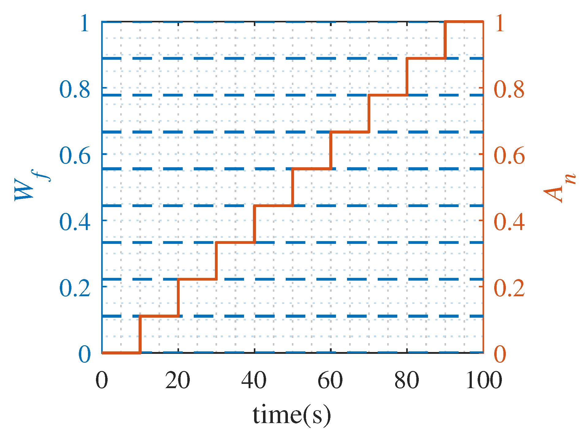
The EM of an MIMO turbofan engine develops from a simple curve to a complex surface form. In the simulation, the engine NCL model works at H = 0 km, Ma = 0. In this paper, input variables of MIMO turbofan engine are fuel flow
and throat area of the nozzle
. At each
, the
increases step by step during simulation. The specific change of input variables is shown in
Figure 1. Then, the high-pressure rotor speed
, low-pressure rotor speed
, and engine pressure ratio (
) are considered to be the output variables of the turbofan engine.
Figure 2,
Figure 3 and
Figure 4 show the output results of the NCL model in simulation. The inputs in
Figure 1 is normalized, and the actual range of
is 1.5906–2.4060 kg/s, while the actual range of
is 0.2577–0.3144
. This process involves the acceleration of the engine. Meanwhile, the steady-state data which is required for the identification of the EME model is extracted from the dynamic process. In addition, all the data in this paper are normalized results.
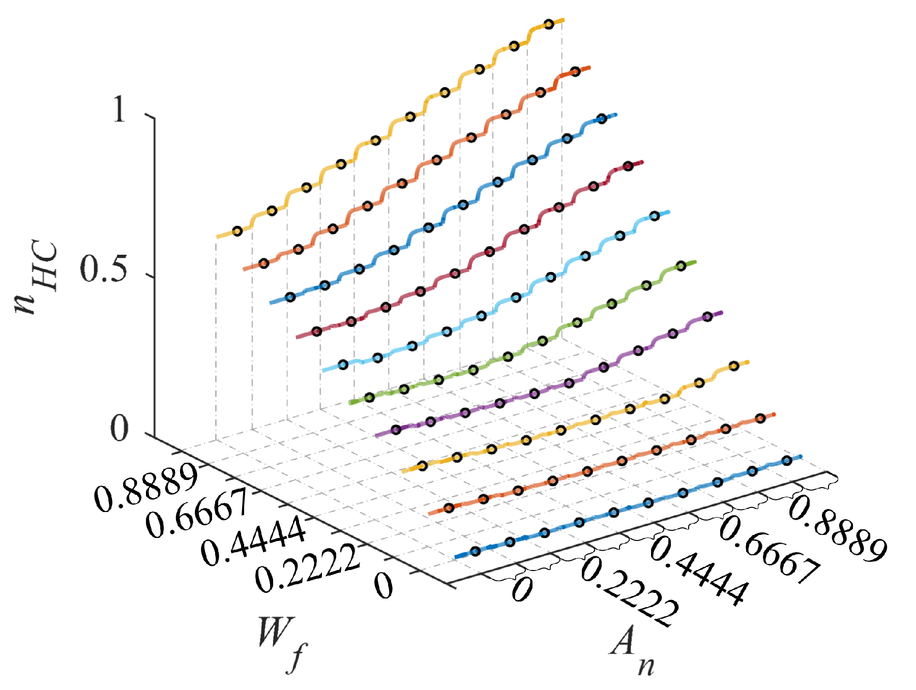
Instead of simple data processing, it is significant to analyze the steady-state and dynamic performances of nonlinear plants and select the appropriate structure for the identification of the EME model. Firstly, when
is small,
is hardly affected by
in
Figure 2. It indicates that the turbofan engine exhibits strong nonlinearity over a wide range of operating conditions. As the value of
reaches around 0.3333,
rises with the increase of
(greater than 0.6667). Subsequently,
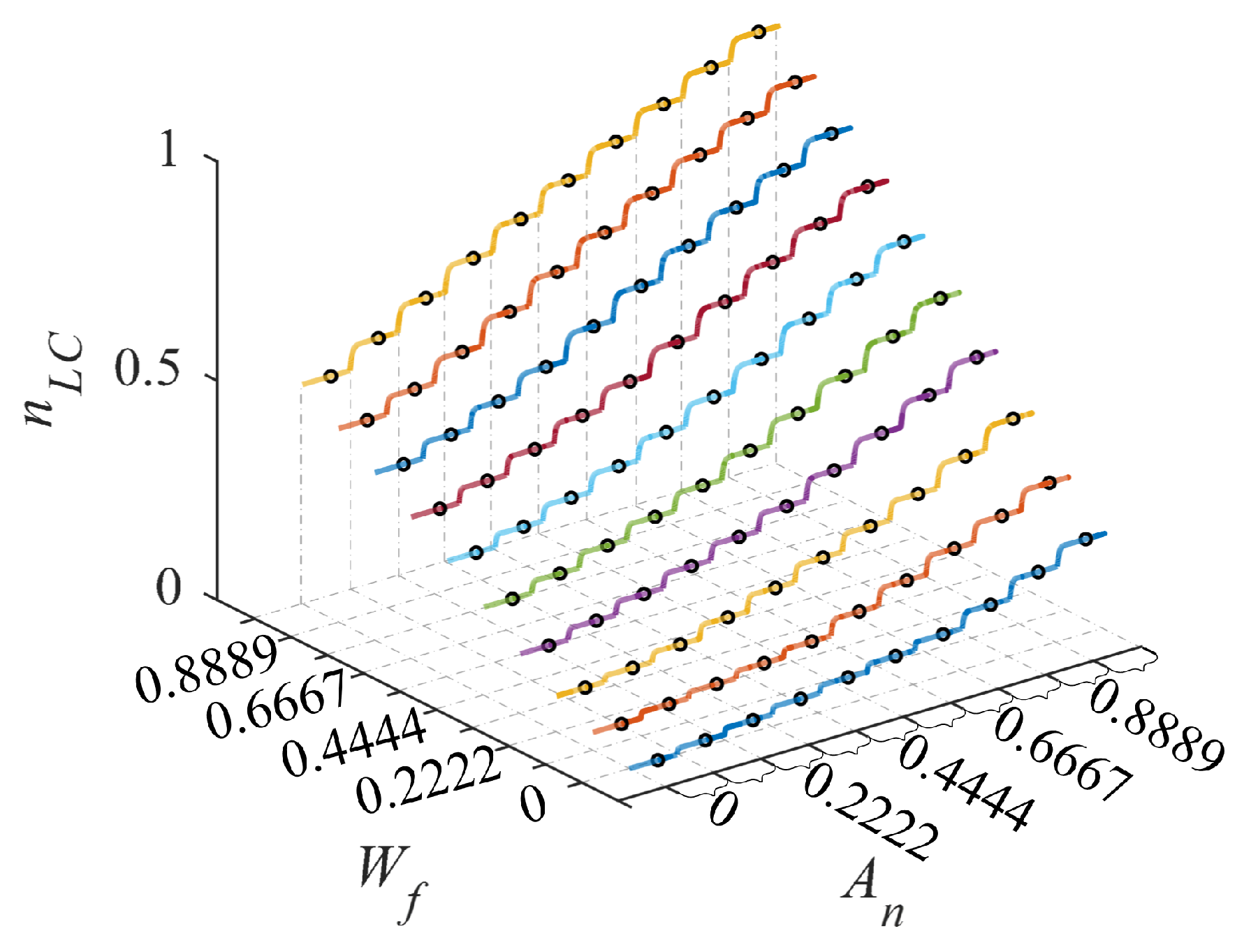
Figure 3 shows that both
and
have effects on
in 10 groups of dynamic operation. On the whole, larger
and
correspond to higher
. As
increases, there appears a prominent steady-state linear relationship between
and
. Next,
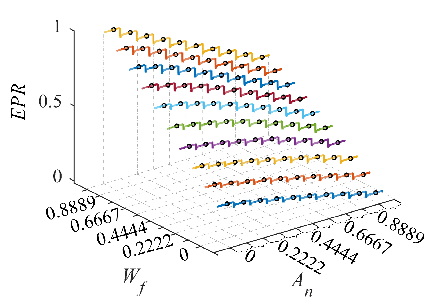
Figure 4 indicates that
effectively regulates the overall work capacity of the turbofan engine. The performance of the engine improves with the increase of
, and
increases at the corresponding
. However, the engine is close to dangerous conditions in high performance, such as surge. Therefore,
plays an important role in solving engine safety problems in high performance operation. Under the same
condition,
can be effectively reduced by increasing
, which provides control direction for avoiding compressor surge.
3.2. Identification of the MIMO EME Model
The turbofan engine is described as follows:
where
is the vector of the state variable,
is the vector of the output variable, and
is the vector of the input variable. In this paper, the typical state variables
and
of turbofan engines are directly used as output variables.
The family of steady-state operating points of this engine is expressed as:
where
.
The EM shown in the Equation (
3) is parameterized by
. Thus, the EME model of the turbofan engine shown in Equation (
4) can be obtained as follows:
where
,
,
,
,
,
.
The number of scheduling variables
in the EME model is equal to the number of input variables. In this section,
and
are selected as
to build the EME model of turbofan engine. So, the structure of
is shown as follows:
According to Equation (
10),
, and
. Meanwhile,
and
are both state variables and output variables. Thus, the EME model of turbofan engine shown in Equation (
9) can be replaced by:
Here, the MIMO EME model of the turbofan engine is established according to Equation (
11). The modeling procedure, which is called the steady-state and dynamic two-step method, is divided into two steps:
Based on the steady-state results obtained by the simulation of the turbofan engine NCL model, the steady-state EM results of the engine shown in Equation (
8) are identified.
In the NCL model simulation process, the input variable signal is set to the staircase signal. The EME model coefficients in Equation (
11) are identified by simulation results of the NCL model and the EM model.
Firstly, it is significant to obtain steady-state EM of turbofan engine for modeling the EME model that shown in Equation (
11). Normally, the EM is identified by polynomial. Considering the accuracy of the identification, the engine EM is identified with the m-order polynomial as shown below.
where
is the EM of the turbofan engine, which is distinguished by the subscript
n.
Table 1 shows the subscript
n corresponding to different EM
.
When
and
are selected as scheduling variables
, the EM of the turbofan engine are
,
, and
, which have the structure of Equation (
12). The one-to-one correspondence between the input variables
and the performance parameters
of the turbofan engine is shown as the black circular mark in
Figure 2,
Figure 3 and
Figure 4. These data are obtained by simulating the turbofan engine NCL model carried out in
Section 3.1. Therefore,
and
are taken as independent variables to extract all steady-state results from simulations, and the corresponding dependent variables
,
, and
are obtained. By using the least square method and selecting the 4-order polynomial
, the identification results of EM
for the turbofan engine are shown in
Table 2. Meanwhile, the comparison steady-state results and error analysis are shown in
Figure 5,
Figure 6 and
Figure 7.
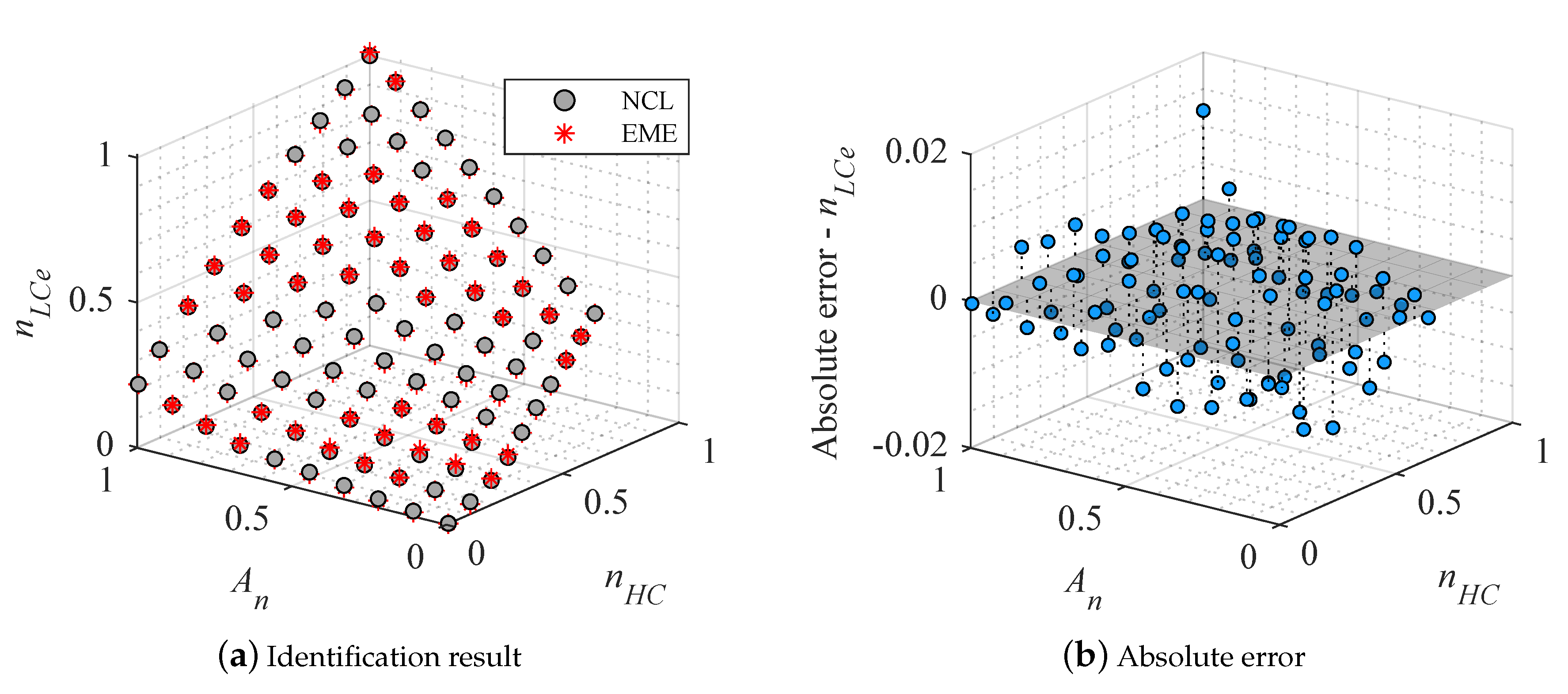
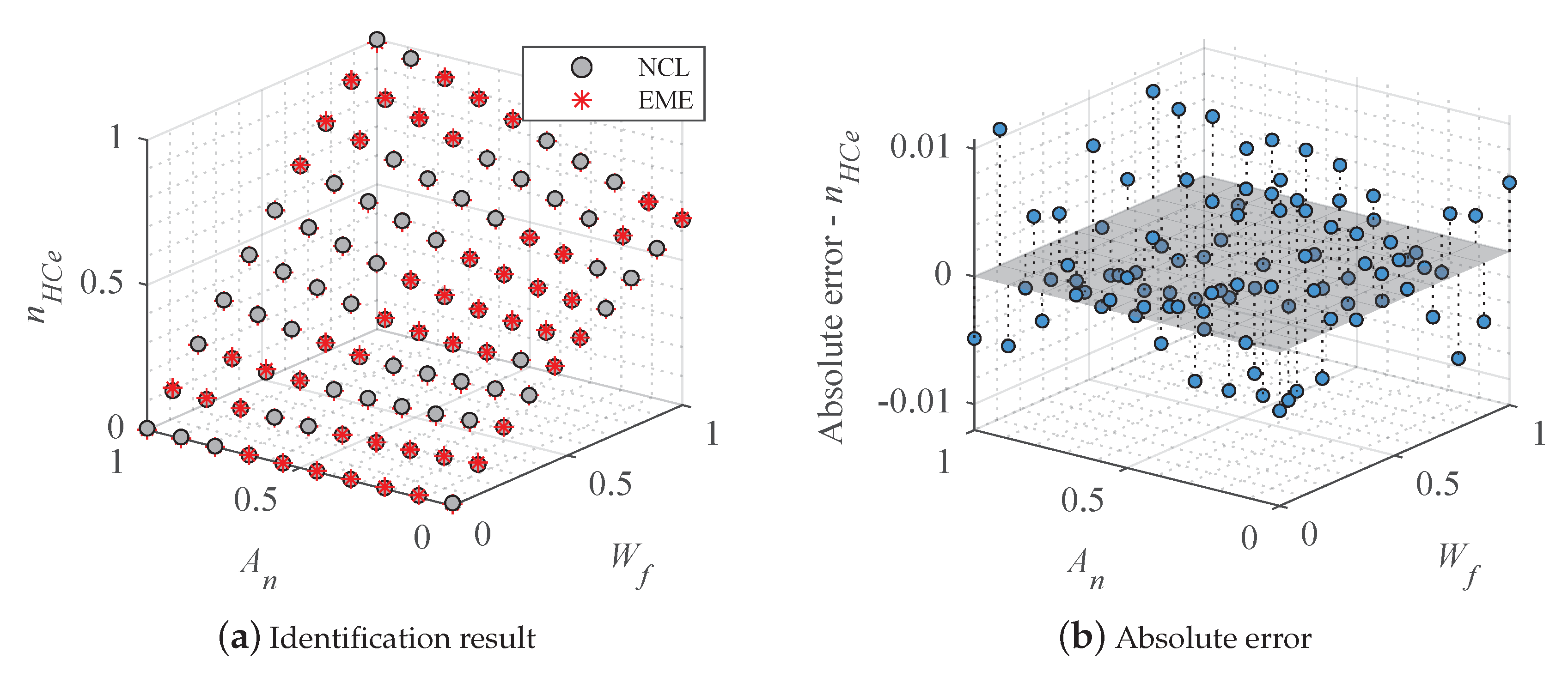
In
Figure 5a,
Figure 6a, and
Figure 7a, the identification results of EM
are presented. Among them, the black points are the steady-state results of the NCL model, and the red asterisks are the fitting result. Meanwhile, the absolute errors of the EM with the NCL model’s steady-state results are given in sub-figure (b). Firstly,
Figure 5 indicates that the absolute error range of
is about −0.015–0.017. In the region composed of
(0–0.4) and
(0–0.5), the fluctuation of the
is caused by the strong nonlinearity of the engine, and the error changes from −0.0084 (
= 0.1034,
= 0) to 0.0168 (
= 0.1885,
= 0.1111) and then to −0.0132 (
= 0.3761,
= 0.1111). The same phenomenon also occurs when
and
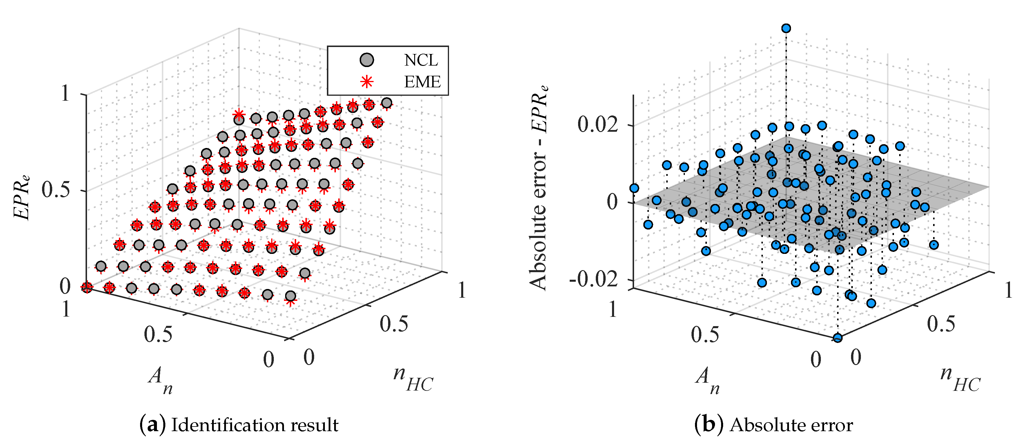
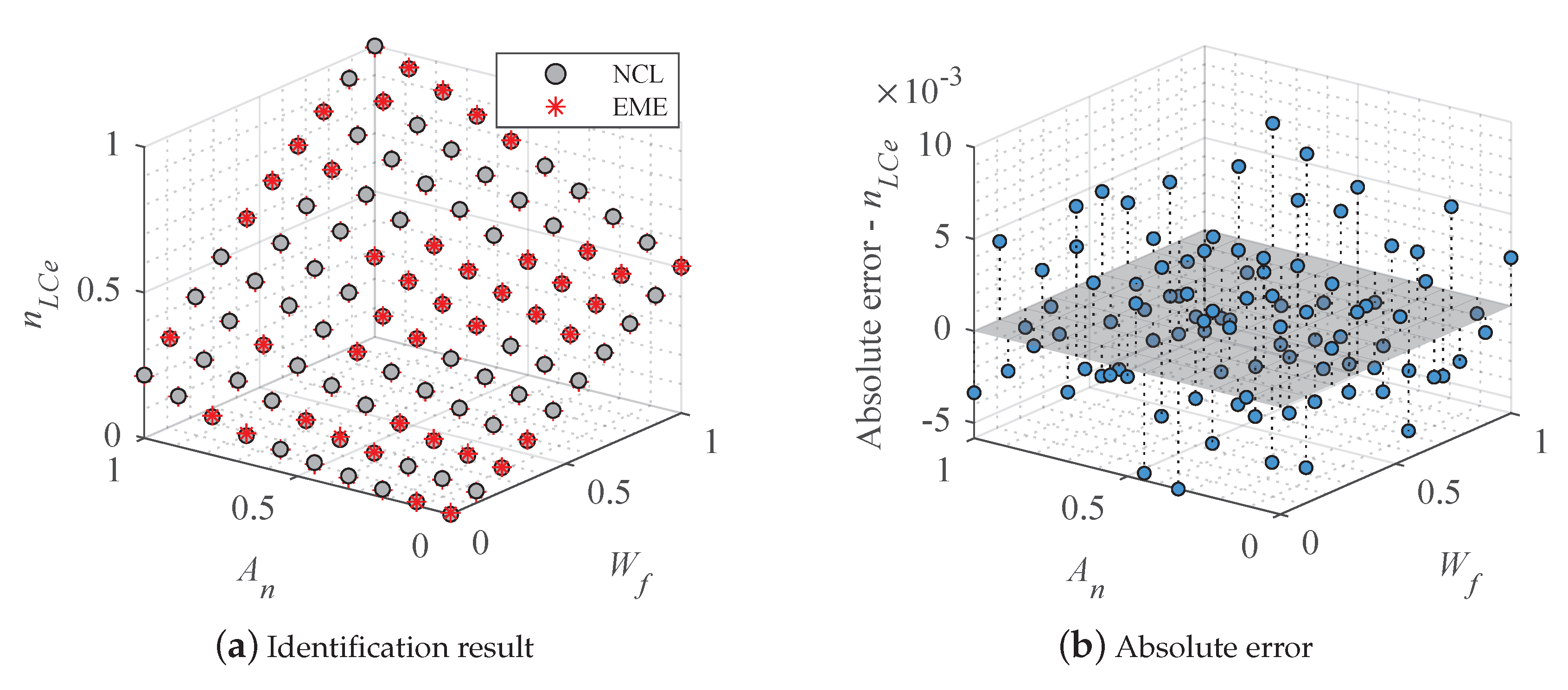
become larger, but the fluctuation amplitude is smaller. Secondly, the absolute error range of
is about −0.022–0.028, and the maximum value is 0.028 (
= 1,
= 1) in
Figure 6. There appears the same strong nonlinear region, in which the error of
changes by a wide margin from −0.0219 (
= 0.009,
= 0) to 0.0196 (
= 0.1885,
= 0.1111) and then to −0.0207 (
= 0.3761,
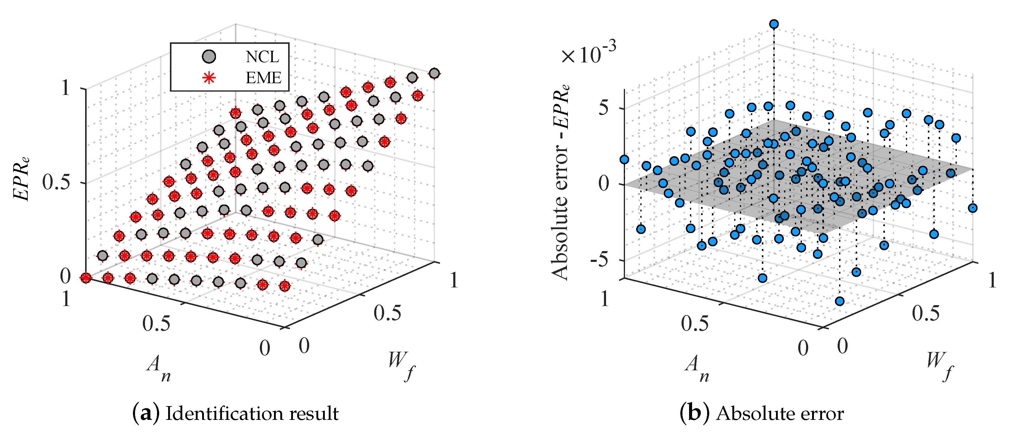
= 0.1111). Thirdly,
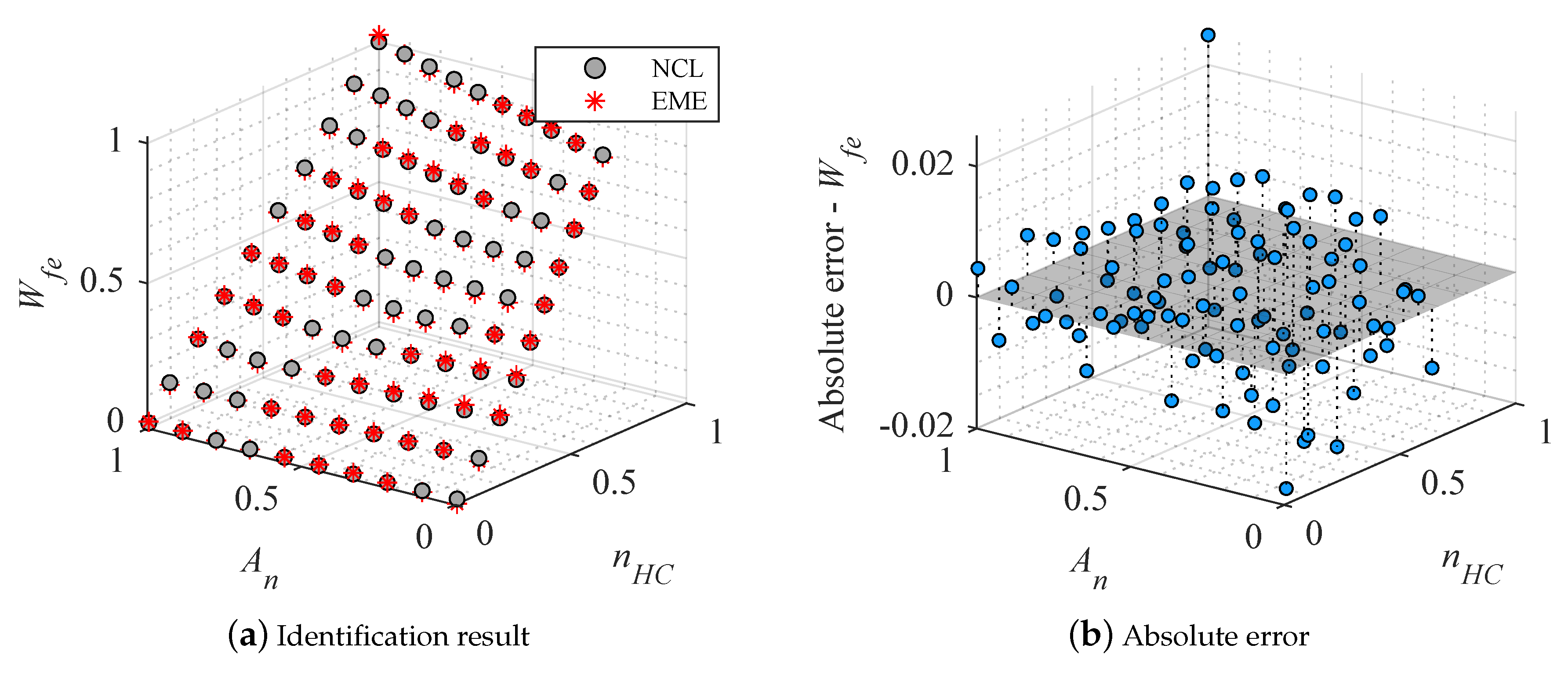
Figure 7 shows the absolute error of
. Its range is about −0.02–0.024, and the maximum one is 0.0246 (
= 1,
= 1). Besides, the absolute error of
changes from −0.0176 (
= 0.009,
=0) to 0.0180 (
= 0.1885,
= 0.1111) and then to −0.0188 (
= 0.3814,
= 0.2222) in the same strong nonlinear region. Overall, the identification result of the
is better than the
, and
, which is less than 0.017.
The fourth-order polynomial used in this section meets requirement of the accuracy. Usually, when a low order polynomial is used to fit the EM of the system with strong nonlinearity, the steady-state accuracy may not be satisfied. It is considered that increasing order of polynomial is a method to improve the fitting accuracy of the EM. However, the EM with a high-order polynomial also brings problems, such as overfitting and complex expression forms, when the result of the EM is close to the data from the NCL model. It is not conducive to the application of the EME model. In addition, the future research can also adopt switching method and neural network to solve the accuracy problem of the EM.
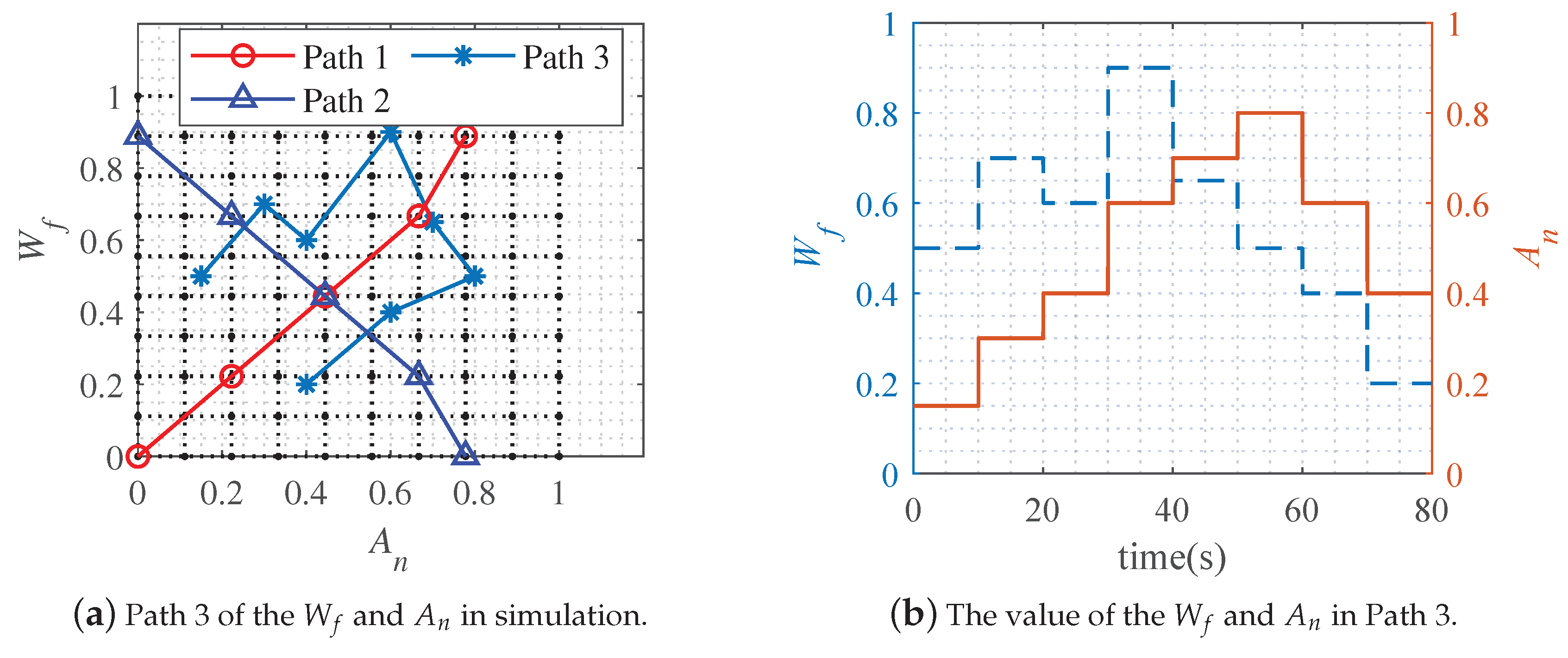
Secondly, the dynamic and static two-step identification method is applied to fit the EME model. After obtaining the steady-state EM, the coefficient matrix
,
,
, and
in Equation (
11) is identified by the dynamic simulation results of the turbofan engine NCL model. In the simulation of the NCL model, the input variables
and
that contain two paths considering the sufficient excitation conditions for the identification are shown in
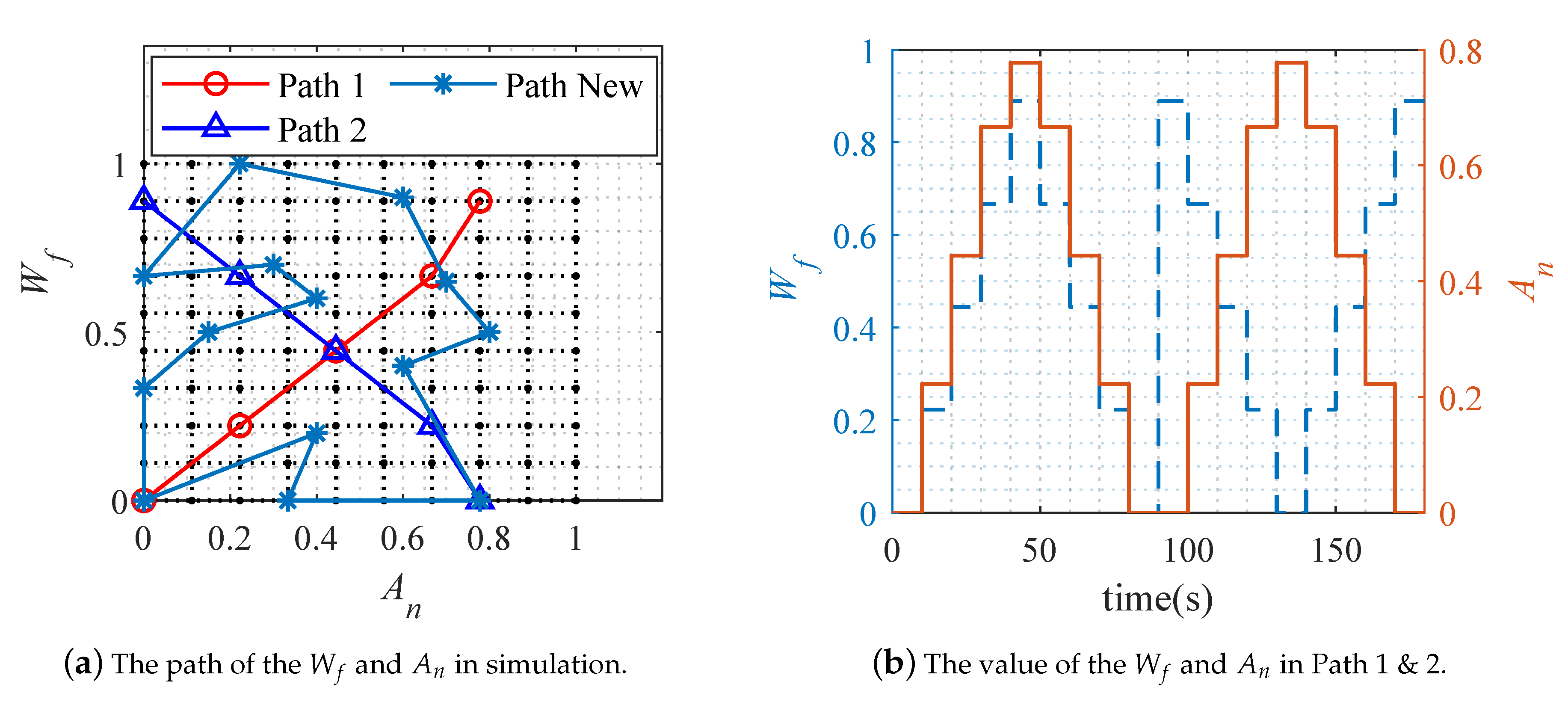
Figure 8. As described above, the identification results of the EM require a large number of steady-state data to ensure the accuracy. However, this is not the case for the dynamic parameters of the EME model. If a large number of dynamic processes are adopted or the variation interval of input parameters is excessively reduced in the identification, the results of EME model may be unstable. Therefore, some simulation paths are provided in
Figure 8a to obtain the data needed for the dynamic coefficients of the EME model. Path 1 and Path 2 are the diagonal lines of the feasible region of the engine input, and they contain a certain degree of dynamic characteristics. However, neither Path 1 nor Path 2 alone can identify stable dynamic parameters of the EME model. This situation is alleviated after combining Path 1 and Path 2 (Path 1 & 2). At the same time, through the well-designed dynamic parameter identification Path New, better identification results are obtained.
Table 3 shows the accuracy results of EME model under different dynamic paths in this paper. Analysis indicators include the sum of squares due to error (
), root mean squared error (
), and coefficient of determination (
). The closer the
and
are to 0, the better the model selection and fitting, and the more successful the data prediction. The closer
is to 1, the better the model fits the data. The results show that the path for dynamic parameters fitting will affect the accuracy of the EME model. Path New has higher accuracy than Path 1 & 2. Facing different engines, a well-designed dynamic path can improve the accuracy of the EME model. The difficulty is that the dynamic path selection is random, and the optimal path for different engines is also difficult to obtain. On the contrary, the combination of Path 1 and Path 2 is the general operating range of turbofan engines. From the results of
Table 3, the EME model identified by Path 1 & 2 has the satisfactory accuracy. Therefore, the study adopts Path 1 & 2 to carry out dynamic parameter identification of EME model, and carries out follow-up work based on this path.
Figure 8b shows the input variables changing along Path 1 (0–90 s) and Path 2 (90–180 s). Thus, the scheduling variables
, derivatives (
), and deviations (
,
) in the EME model of the turbofan engine can be obtained. That is,
,
,
, and
in Equation (
11) can be calculated by the NCL and EM simulations. The coefficient matrix of the EME model is identified as follows:
The identification results of Equation (
13) are shown in
Table 4.
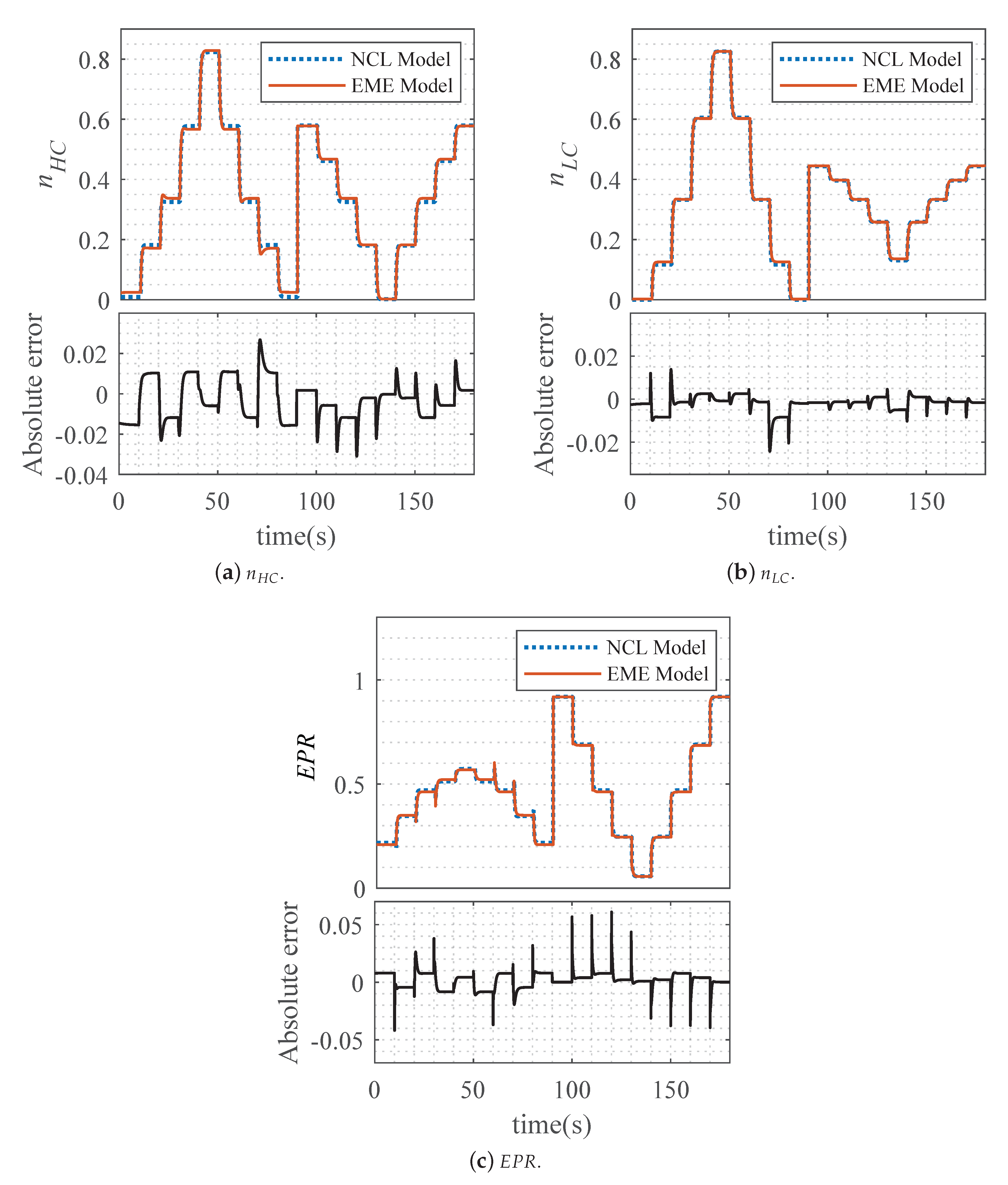
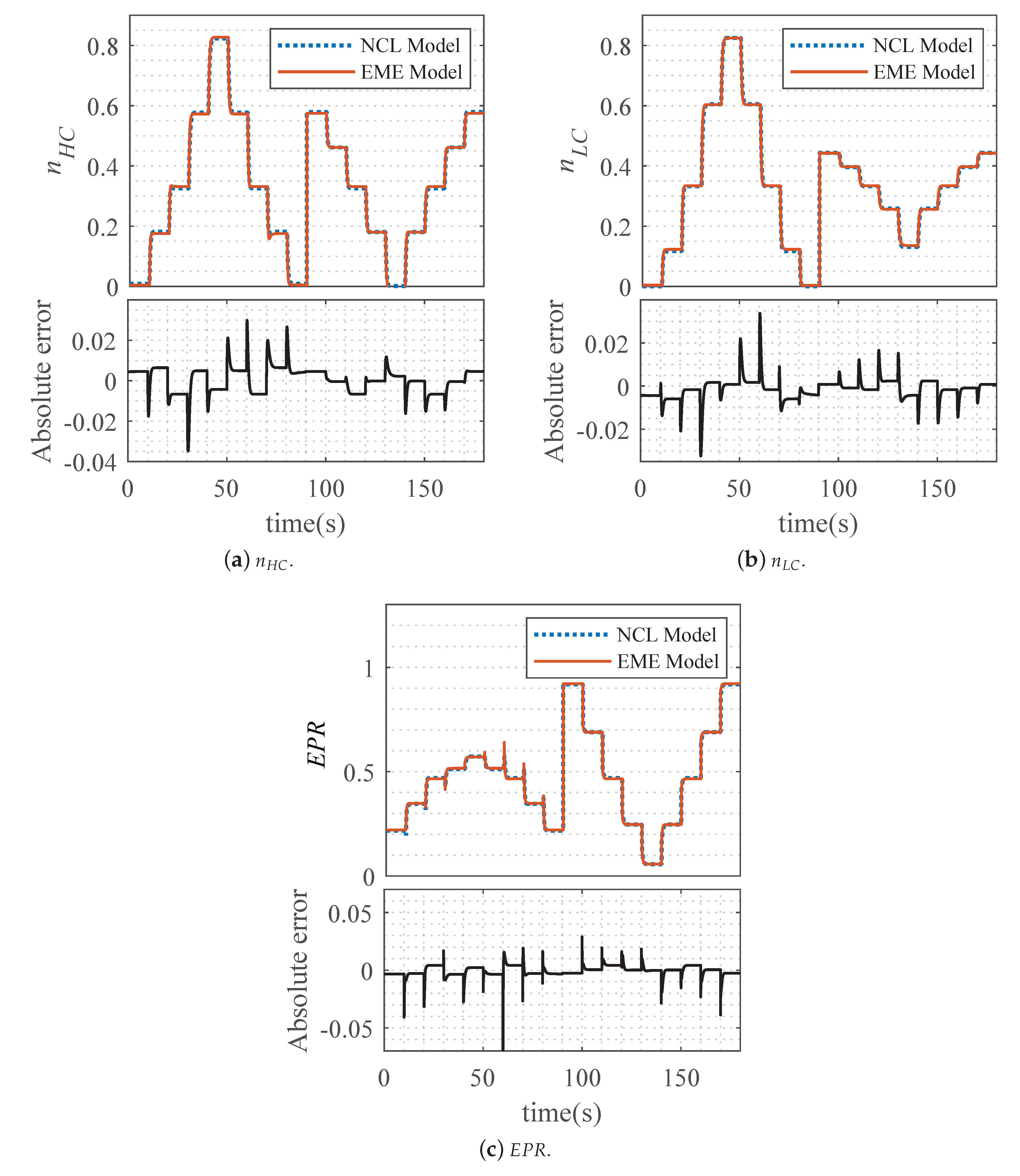
So far, all the parameters of the EME model have been identified. Naturally, it is necessary to validate the accuracy of the EME model. During the verification, the input variables
and
are still shown in
Figure 8. In addition, the comparison and error analysis of the turbofan engine’s NCL model and EME model are shown in
Figure 9. The results given by
Figure 9 show that the
and
of the EME (
) have high steady-state accuracy, while the
has low steady-state accuracy. Obviously, the steady-state accuracy of
and
is determined by the identification results of
and
, respectively. Meanwhile, the simulations also indicate that the
and
meet high dynamic accuracy, in which the dynamic time of the EME model is similar to that of the NCL model. In particular, there appears a dynamic error with absolute value around 0.02 for the simulations of
at 10 s and 70 s in
Figure 9b. In
Figure 9c, the results of
show a dynamic error with absolute value around 0.05. The large dynamic error of the
may be caused by the negative regulation characteristics. However, the
shown in
Figure 9a is not satisfactory. In the simulation, large overshoot occurs in the EME model at 20 s, 60 s, and 70 s, and the overshoot at 70 s is close to 0.02.
3.3. Effects of Scheduling Variables on Model Accuracy
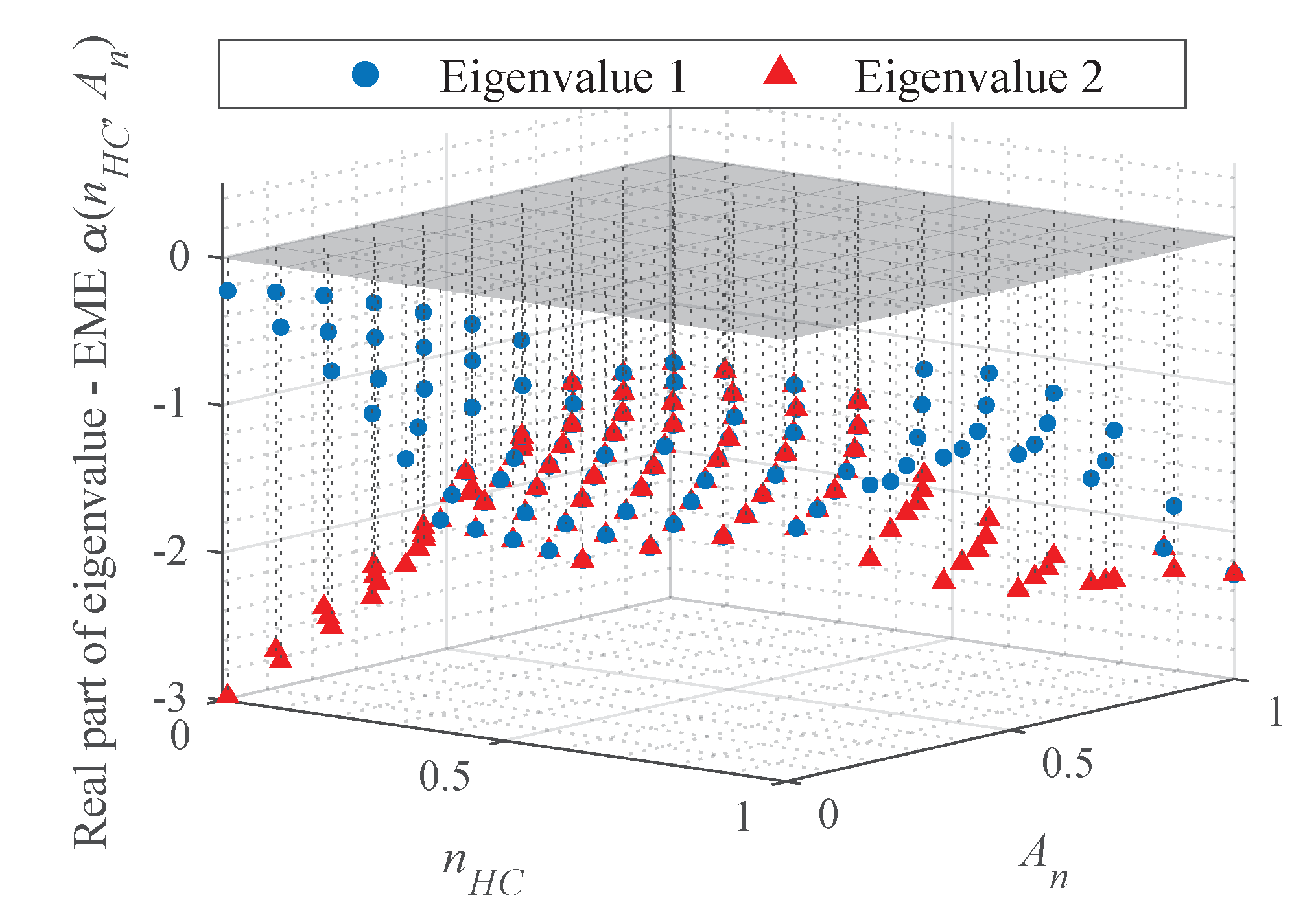
In
Section 3.2, there are some errors in the steady-state and dynamic accuracy of EME (
) model, especially in
. Thankfully, the previous studies have shown that the optimal identification form of the EME model always exists in the nonlinear plants with analytic representation. Although MIMO turbofan engine with strong nonlinearity cannot be expressed analytically, the accuracy of the EME model can also be improved by selecting different combinations of the scheduling variables.
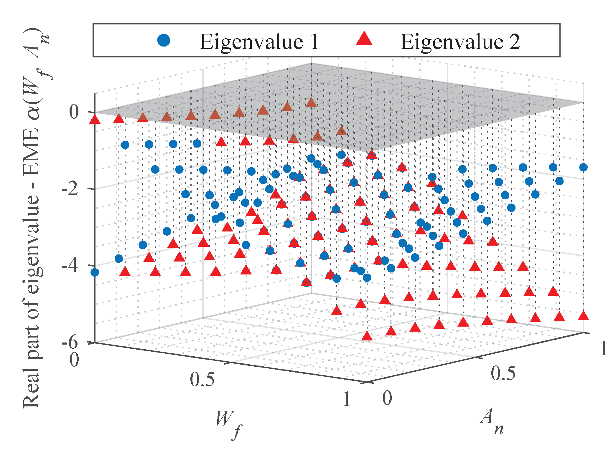
and
are selected as
to complete the EME model of the turbofan engine in this section. Thus, the form of
can be rewritten as follows:
According to Equation (
10),
, and
. Thus, the EME model of the turbofan engine shown in Equation (
9) can be replaced by:
Firstly, we identify the EM of the turbofan engine. When
and
are selected as scheduling variables
, the EMs of the turbofan engine are
,
, and
which meet the form of Equation (
12). Based on the method given in
Section 3.2, the identification results of steady-state EM are shown in
Table 5. Meanwhile, the steady-state results and the absolute error analysis of EM with NCL model are shown in
Figure 10,
Figure 11 and
Figure 12. The identification results of EM (
) are presented in
Figure 10a,
Figure 11a, and
Figure 12a. Among them, the black points are the steady-state results of the NCL model in
Section 3.1, and the red asterisks are fitting results. The absolute error of the EM with the NCL model’s steady-state results is given in
Figure 10b,
Figure 11b, and
Figure 12b.
Clearly, the operating range of the
is shown in
Figure 10, and the maximum absolute error is −0.0120
. However, the strong nonlinear region of the EM in EME (
) is not significant in EME (
).
Figure 11 shows that the absolute error range of
is about −0.006–0.010. The extremum of the absolute errors are −0.0058 (
) and 0.0098 (
) in
Figure 11b. In addition,
Figure 12b indicates that the absolute error range of
is about −0.0060–0.0060. The extremum of the absolute errors are −0.0061 (
) and 0.0040 (
) in
Figure 12b. In general, the accuracy of the EM in EME (
) is higher than in EME (
).
Secondly, the coefficient matrix
,
,
and
in Equation (
11) is identified by the dynamic simulation results of the turbofan engine NCL model. Clearly, the specific fitting method is given in
Section 3.2. That is,
,
,
, and
in Equation (
15) can be calculated by the results of the NCL model and the EM. The coefficients of the EME model can be identified as follows:
Therefore, the identification results of Equation (
16) are shown in
Table 6.
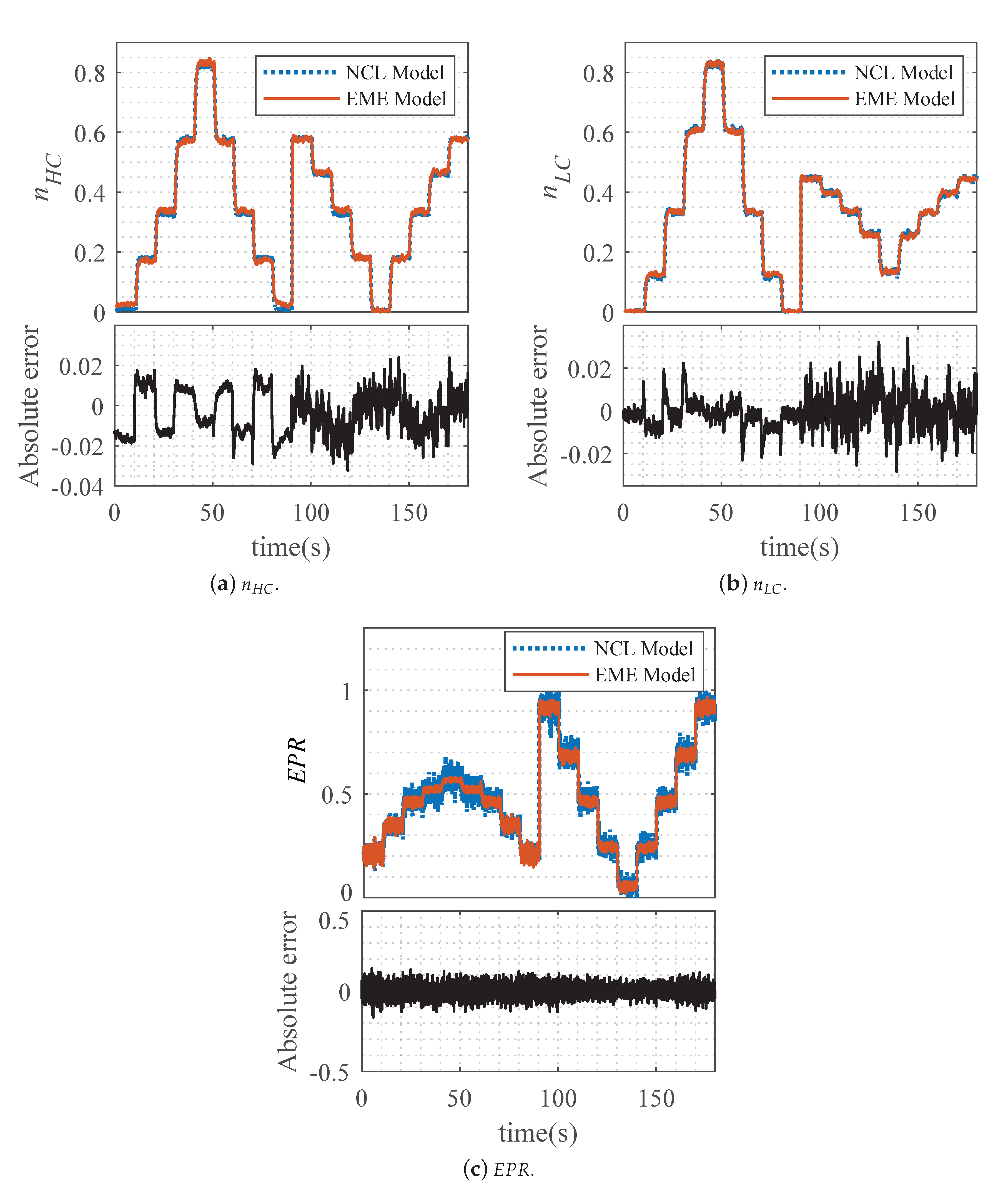
Because the validation is an important part of modeling, so the validation of the EME model is carried out as follows. The input variables
and
vary according to the rule shown in
Figure 8. Through the simulation, the comparison and error analysis of the turbofan engine’s NCL model and EME model are shown in
Figure 13. The results demonstrate the accuracy of the EME model along the design Path 1 & 2.
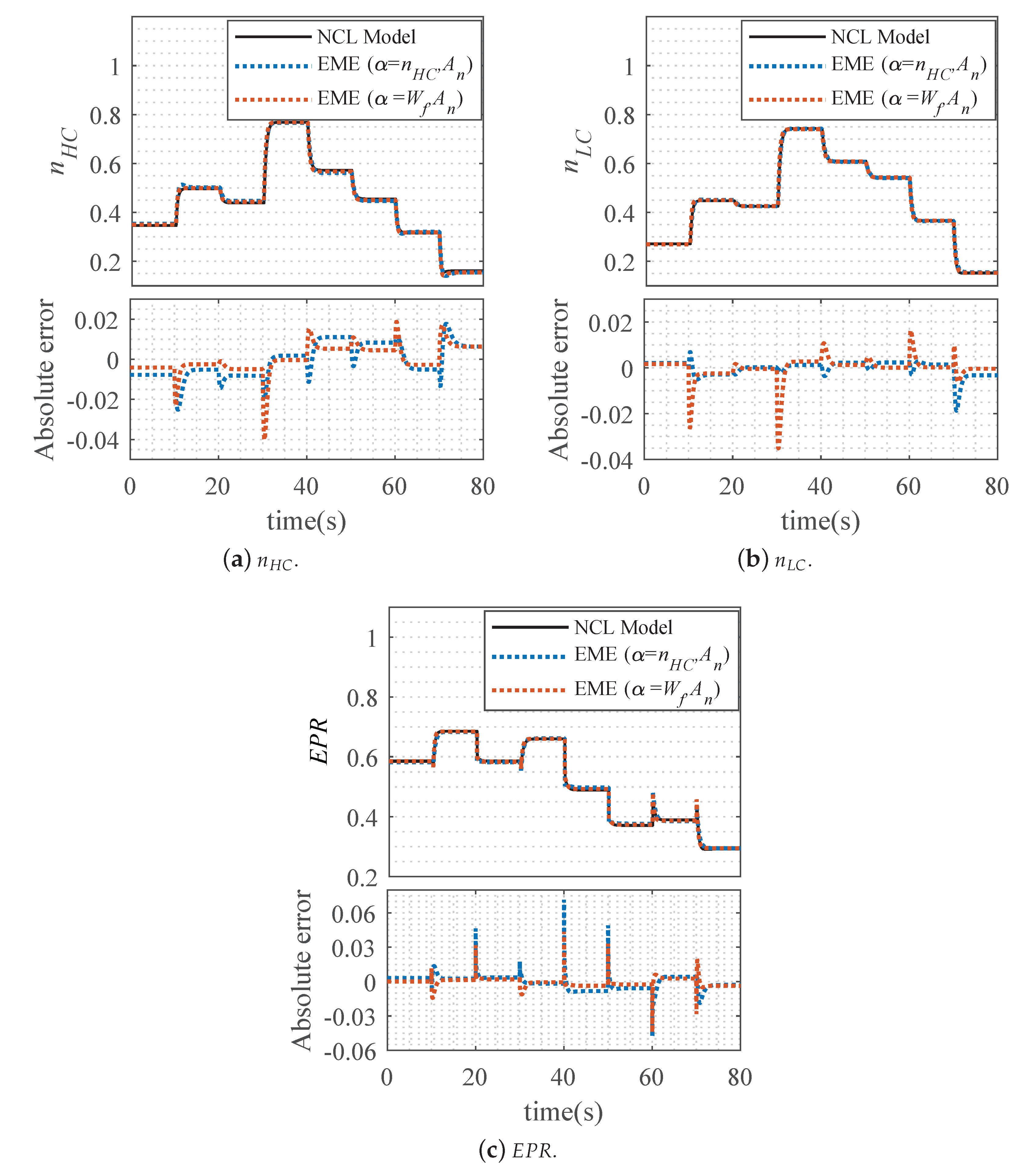
Figure 13 indicates that
,
, and
in EME (
) all have high steady-state accuracy, which is determined by the identification results of the EM. Simultaneously, the results also have high dynamic accuracy in EME (
). There are large dynamic errors for
,
, and
at 60s, and the values are 0.025, 0.0275, and −0.055, respectively. The EME (
) model can reflect the overshoot characteristics of
in the range of 0–0.035. Besides, the overshoot is less than the EME (
) at 60 s in
Figure 13a. The accuracy of the EME model is affected by
, which is confirmed in the simulation. The analysis indicators in
Table 3 shows that the EME (
) model has higher steady-state accuracy than the EME (
) model, and the identification result of the
is more satisfactory. However, direct measurement of inputs, such as real engine fuel, will limit the feasibility of inputs as scheduling variables for the EME model.


