Abstract
A sliding mode control (SMC) technique based on a state observer with a Kalman filter and feedforward controller was established for a variable-speed refrigeration system (VSRS) to ensure robust control against model uncertainties and disturbances, including noise. The SMC was designed using a state-space model transformed from a practical transfer function model, which was derived by conducting dynamic characteristic experiments. Fewer parameters affecting the model uncertainty were required to be identified, which facilitated modeling. The state observer for estimating the state variables was designed using a Kalman filter to ensure robustness against noise. A feedforward controller was added to the control system to compensate for the deterioration in the transient characteristics due to the saturation function used to avoid chattering. A genetic algorithm was used to alleviate the trial and error involved in determining the design parameters of the saturation function and select optimal values. Simulations and experiments were conducted to verify the control performance of the proposed SMC. The results show that the proposed controller can realize robust temperature control for a VSRS despite stepwise changes in the reference and external heat load, and avoid the trial and error process to design parameters for the saturation function.
1. Introduction
Variable-speed refrigeration systems (VSRSs) are widely used in various industrial fields due to their excellent energy-saving ability and high-precision temperature control capability [1,2,3,4,5,6,7]. VSRSs, which are composed of a variable speed compressor, an electronic expansion valve (EEV) and heat exchangers, have inherent nonlinear characteristics. Consequently, it is challenging to perform linear approximation modeling for VSRS controller design. Even a sophisticated numerical model in the form of a high-dimensional linear state-space model encounters difficulties in the suitable design of a VSRS control system due to the model uncertainties and disturbances, including noises. Moreover, accurate identification of the system parameters in high-dimensional models for VSRSs is extremely laborious and tedious. Therefore, a control method that is based on a low-dimensional practical model for VSRSs and is robust against model uncertainties and disturbances must be formulated.
The target temperature in VSRSs is controlled by regulating the mass flow rate of the refrigerant according to the change in the compressor rotation speed. Moreover, the superheat is controlled by adjusting the EEV opening angle to prevent adverse effects such as a decrease in the coefficient of performance (COP) due to superheated vapor compression and liquid back phenomenon. Therefore, the control system for a VSRS can be considered a multiple input/output (MIMO) system [1,2,3,4,5,6,7]. Temperature control methods for VSRSs can be divided into two groups based on the requirement of a mathematical model, and include model-based control and artificial intelligence (AI) technology control methods. Model-based control techniques can be divided into transfer function model-based and state-space model-based approaches, the representative controllers of which are proportional–integral–derivative (PID) and optimal control, respectively. A PID controller is easy to design and implement for a single input/output system (SISO), and exhibits a relatively high control performance when the nominal model is correct [1]. However, it is difficult to ensure control robustness against model uncertainties because the PID gain is generally designed considering a nominal model. Optimal control strategies, such as those based on a linear quadratic regulator and linear quadratic Gaussian, are suitable to design controllers for MIMO systems and ensure optimality by balancing the control accuracy and input energy. However, such controllers also cannot ensure robustness against model uncertainties and disturbances [3,8,9,10]. Notably, fuzzy control, which is an AI technique, does not require the dynamic model of a plant when designing the control system. Therefore, fuzzy control is suitable for VSRSs, for which the establishment of a linear model is challenging due to their high nonlinearity. However, this control method is expensive because it requires a high-performance microprocessor to promptly calculate large amounts of logic when precise control is necessary. In particular, the systematic design of this control method is difficult because the design of the membership function and rule base, which are key components in the fuzzy controller, is excessively dependent on the knowledge and experience of experts [6,7,11]. Hence, model-based control that does not rely on the plant parameters is desirable for systematic robust controller design.
As a dynamic model of VSRSs used to realize model-based control, an analytical model derived by applying the governing equation of Navier–Stokes to a heat exchanger was proposed [12]. Because this model is a high-order nonlinear partial differential equation, model uncertainty is generated in the process of linearization and low-dimensional modeling, and the model uncertainty increases in the process of parameter identification of the model. Another method to obtain a low-dimensional model is to transform a practical transfer function, obtained through dynamic characteristic experiments, into a state-space model [1]. However, conventional control methods such as PID controllers based on this model cannot ensure control robustness because the model uncertainty increases under an operating environment that is different from the experimental environment considered to obtain the nominal model. In summary, model-based control, such as PID or optimal control, is not adequately robust, because the performance of the designed controller is considerably deteriorated by the model uncertainty of the nominal model and the inflow of disturbance, including noise. Therefore, it is desirable to design a controller for which the gain does not depend on the parameters of the nominal model in order to ensure the precise temperature control of VSRSs. Sliding mode control (SMC) has attracted considerable attention as a robust control method to solve this problem. The SMC is based on variable structure control: the structure of the control system is changed, and the sliding mode is realized on the designed sliding plane (or line). Because the discontinuous control input of the SMC is independent of the system parameters of the nominal model, this control method is robust against model uncertainties and disturbances [13,14,15,16].
Although many researchers have attempted to apply SMC to the servo control of AC motors and robots, research on the application of SMC to heating, ventilation, and air conditioning (HVAC) systems remains limited. The existing studies on the use of SMC for VSRSs have adopted complicated high-dimensional analytical models, and either the temperature control performance was not precisely verified experimentally or the main objective was not temperature control [17,18,19]. Certain authors have adopted SMC with an optimal switching hyperplane for an HVAC system using a high-dimensional state-space model, obtained by applying the moving boundary model to heat exchangers [17]. However, the model was verified only through simulations, and the evaluation functions essential for optimal control design were not explicitly presented. Other researchers applied the SMC for variable-air volume air-conditioning systems to optimize the energy consumption and control temperature [18]. However, the model used to design the controller was not clearly explained, and the control performance of the SMC was evaluated only through simulations. SMC was also applied for automotive air-conditioning/refrigeration systems to achieve energy savings [19]. However, this study focused on only the energy saving performance, and not high-precision temperature control. Moreover, the verification of this method can be considered inadequate because the performance of the proposed controller was evaluated by comparing it to conventional on/off control.
Considering this aspect, this paper proposes an SMC with a two-dimensional phase plane for a VSRS that is based on a low-dimensional practical state-space model. Using this approach, the proposed controller can render the behavior of state variables intuitively understandable, and enhance the control performance. Moreover, the number of parameters to be identified, which can increase the model uncertainty, is significantly reduced, and modeling is facilitated. The state observer is composed of a Kalman filter to ensure robustness against process and observation noise. To suppress chattering due to the switching function, which is a notable problem in SMC, a saturation function is used instead of a signum function. Moreover, a feedforward controller is designed to avoid the deterioration in the transient characteristics of the main controlled variable due to the use of this saturation function. Furthermore, the genetic algorithm (GA) is used to avoid the cumbersome trial and error process for determining the design parameters of the saturation function, which influence the control performance, and for selecting the optimal values [20,21,22,23,24]. The validity of the proposed controller is verified through simulations and experiments with a VSRS-based oil cooler system (OCS) as the plant. In addition, the effectiveness of the suggested controller is demonstrated by comparing the control performance with that of a conventional proportional–integral (PI) controller.
2. Design of SMC with Kalman State Observer
2.1. Two-Dimensional State-Space Modeling for VSRS
Figure 1 shows the schematic of a VSRS-based OCS composed of a variable speed compressor, an EEV, and heat exchangers. The OCS prevents the thermal deformation of the workpiece and the deterioration of the processing precision by supplying oil at a constant temperature to promptly remove the unnecessary heat generated in the machining area of precision machine tools. Moreover, the OCS controls the irregular temperature of the oil returned from the machine tools in order to maintain a constant temperature by changing the rotational speed of the compressor and adjusting the mass flow rate of the refrigerant. The superheat is simultaneously controlled to prevent a decrease in the COP due to overheated vapor compression and compressor failure due to liquid back caused by a rapid change in the compressor speed.
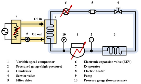
Figure 1.
Schematic of the oil cooler system based on the VSRS.
Figure 2 is a block diagram showing the input/output relationship used to obtain the transfer function models of the compressor and EEV.
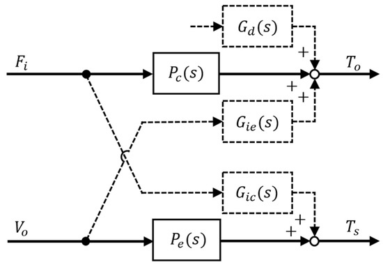
Figure 2.
Input and output variables of the transfer functions for a compressor and EEV.
In the design of the SMC, the main controlled variable of the OCS is the oil outlet temperature , and the auxiliary controlled variable is the superheat . The control inputs (manipulated variables) for the two controlled variables are the references of the inverter frequency and EEV opening angle , respectively. The transfer functions and , indicated by solid lines in Figure 2, are dynamic characteristic models of the compressor and EEV, respectively, which are the control objects. The transfer functions and , indicated by dotted lines, represent the mutual interference effect between the controlled variables. In other words, these functions represent the effects of the change in on , and of the change in on . The transfer function represents the effect of a change in the heat load, which is a disturbance, on . The two transfer functions and are used to strictly simulate the dynamic characteristics of the OCS system during simulation, and are not considered when designing the controller.
Equation (1) presents the transfer functions obtained from the dynamic experiments of the OCS, in which the variables and are varied near the operating point to obtain the transfer function , shown in Figure 2. In this experiment, the manipulated variable causing the interference, and not the main manipulated variable, is fixed as a constant . According to Equation (1), the transfer function is a typical first-order system with dead time [1].
Equation (2) indicates the behavior of in the context of a variation in the heat load, which is a disturbance. Moreover, Equation (3) reflects the interference effect of the change in the inverter frequency corresponding to the rotational speed of the compressor on . The parameters are obtained through the dynamic characteristic experiments of the OCS near the operating point. shown in Figure 2 is excluded from the simulation as its effect can be ignored, because this study focuses on designing a controller that is robust to model uncertainties including disturbances, rather than a non-interference controller [6,7].
The two-dimensional state-space model of the OCS used to design the SMC can be expressed as in Equations (4) and (5) in a controllable canonical form, which is easy to analyze and can facilitate the design of the control system. The controllable canonical form is obtained through an inverse Laplace transform applied on the transfer function expressed as a linear quadratic system, by applying a Pade first-order approximation to the dead time component in Equation (1).
Notably, the state variable is a virtual physical quantity obtained in the process of conversion to the controllable canonical form. In addition, the output does not directly refer to the controlled variables and . The functions of time of the state variable , output variable , and control input , etc., are omitted for the convenience of notation.
2.2. Design of SMC with Kalman State Observer
Figure 3 shows a two-dimensional phase plane to illustrate the control principle of the SMC. In Figure 3a, the state variables and are converged to origin along the sliding surface by the SMC. Figure 3b shows the phase plane of the SMC for the servo system. The servo system is constructed by replacing and with the control error and its derivative , respectively. is the set value of .
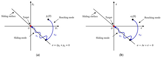
Figure 3.
Phase plane of sliding mode control. (a) Theoretical phase plane. (b) Phase plane for servo system.
The sliding function for a two-dimensional space is generally set as . In this case, is the gradient of the sliding line and indicates the speed at which converges to zero. The sliding function is designed as in Equation (6) by replacing the state variable with . Therefore, the sliding function is a scalar value. In particular, and , because this study focuses on realizing a servo system for precise temperature control, in which based on the SMC.
The control input of the SMC that controls and is generally designed, as in Equation (7), as the sum of the continuous control input for the sliding mode and the discontinuous control input for the reaching mode.
Because is a sliding mode input, it is obtained from when in Equation (6). To determine to control To, Equation (4) is transformed into a generalized expression, as in Equation (8).
Equation (9) is obtained by reflecting the result of Hankel’s singular value decomposition to analyze the contribution of the state variable to the output in the output equation of Equation (8).
Moreover, because , . in Equation (10) is obtained by substituting and from Equation (6).
Equation (11) is obtained from Equation (10), considering the fact that the used for controlling and is defined as the control input at . for controlling is obtained in the same manner as in the case of control. Finally, for controlling and is derived as in Equation (12), by substituting the parameter values of the system defined in Equations (4) and (5).
The discontinuous control input for the compressor and EEV is designed as in Equation (13) from Lyapunov’s second law as the reaching law. The coefficient represents the switching gain, which is generally obtained by trial and error. The signum function is defined as in Equation (14).
Notably, in Equation (12) is linked to the parameters of the system; however, in Equation (13) is independent of the system parameters. forcibly constrains the state variables to the sliding line when the state variables of the system deviate from the sliding line due to disturbances or model uncertainties. Consequently, the SMC exhibits robust control performance despite the uncertainty in the nominal model and the presence of disturbances, including noise, in the control system.
The designed SMC servo control system satisfies the Lyapunov stability condition. According to the Lyapunov stability condition, for any Lyapunov function , if , then the designed control system is asymptotically stable. First, the Lyapunov function for the sliding function A is defined as in Equation (15), and when it is differentiated, Equation (16) is derived.
Substituting Equation (10) into Equation (16), Equation (17) is obtained, so is satisfied.
in Equation (12) requires information regarding the state variable . However, is a virtual physical quantity generated by converting the model of the plant into the controllable canonical form presented in Equations (4) and (5). Therefore, these values are estimated instead of being detected by designing a state observer for control. The state observer consists of a Kalman filter that is robust against the process and measurement noise pertaining to the output variable and state variables of the compressor and EEV. The design of the Kalman filter targets the linear system of Equation (18), including the process noise and measurement noise , which are assumed to be white noise, and represents the problem of estimating the minimum mean square error of state from output . In this case, , and in Equation (18) are the matrices defined in Equations (4) and (5), which represent state-space models.
Equation (19) indicates the state observer to which the Kalman filter is applied. The superscript indicates the estimated value, and is the gain of the Kalman filter obtained from [25,26,27]. Matrix is obtained from the Riccati equation presented as Equation (20), in which and are the power spectral densities of and in Equation (18), respectively.
Notably, in Equation (13) causes chattering in the control input and controlled variable due to the signum function indicated in Equation (14). The saturation (sat) function presented in Equation (21) with the boundary layer thickness is used to alleviate this adverse effect.
The saturation function degrades the transient response of the oil outlet temperature due to , especially when a disturbance is applied. To enhance the transient response of , a feedforward controller is designed, as in Equation (23), by estimating the disturbance presented in Equation (22). The coefficient represents the gain of the feedforward controller, which is generally obtained by trial and error.
Therefore, the final control input for the precise control of the main controlled variable is designed as in Equation (24) by adding Equations (7) and (23). , which is the auxiliary controlled variable, is simply designed as , and the feedforward controller is omitted.
Figure 4 shows the MATLAB/Simulink-based simulation and experimental block diagram of the SMC with the Kalman state observer and feedforward controller to control the compressor. The block diagram for the EEV has the same structure as that shown in Figure 4, except for the feedforward control part used to calculate input .
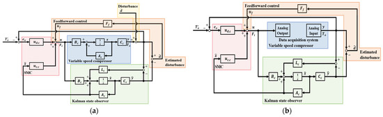
Figure 4.
MATLAB/Simulink program for simulations and experiments to control . (a) Simulation. (b) Experiment.
2.3. Optimization of SMC Based on the GA
The saturation function is applied to suppress the occurrence of chattering due to the signum function of the discontinuous control input. The saturation function involves two design parameters: and . The determination of these parameters to reduce chattering and enhance the control performance requires considerable trial and error. In particular, finetuning must be performed to set the SMC parameters to satisfy the design specifications, which is laborious and tedious. In addition, the design parameters determined through repeated fine adjustments may not be optimal values. Therefore, the GA is utilized to reduce the cumbersome trial and error involved in determining the design parameters of the saturation function and setting the optimal values. Specifically, the GA is applied to optimize the gain of the discontinuous control input in Equation (13) and the of the saturation function in Equation (18) for controlling , which is the main controlled variable. The design parameters to control superheat are determined by the designer through the conventional trial and error method, without applying the GA, as this physical quantity is accessorily controlled.
The GA is an optimization algorithm that simulates the natural evolution process through a computer. The GA represents a global search method in which crossover and mutation are arbitrarily performed, and it exhibits an excellent search capability in a vast problem space [20,21,22]. In addition, the GA is a probabilistic optimization technique and has been applied to many fields, such as parameter estimation and the control of dynamic systems. Figure 5 shows the process flow, indicating the main process of the GA. In the GA, this process is performed until the termination criteria are satisfied, and the optimal solution is derived from the population.
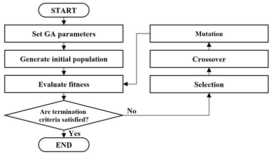
Figure 5.
Process flow of the GA.
First, the objective function of the GA for optimizing the SMC parameters is selected. In general, the integral square error, integral of the absolute error (IAE), integral time square error, and integral time absolute error are widely used as the objective functions of the GA. In this study, IAE, which is a suitable objective function for the temperature control of the VSRS, is used [28], as indicated in Equation (22):
In the GA, constraints are imposed to satisfy the design specifications of the controller, including the settling time s and undershoot °C, which represent the transient characteristics of . The population size is set as 50 and generation is set as 20. As the selection rule, roulette, which increases the probability of selection in the next generation in proportion to the fitness evaluated by the objective function, is adopted. For the crossover, the arithmetic crossover method is used. As the method of mutation, the adaptive possibility approach is applied. Adaptive possibility is a rule that involves the mutation of rates according to the distance, based on the result of measuring the degree of approximation of two individuals generated by the crossover.
Table 1 summarizes the designed SMC and parameters for the saturation function that have been optimized by the GA.

Table 1.
Designed parameters and gains of SMC with feedforward controller.
3. Results of Simulations and Experiments
3.1. Results of MATLAB/Simulink Simulations and Experiments
Figure 6 shows the schematic of the OCS experimental device composed of the VSRS to validate the designed controller. Table 2 and Table 3 present the specifications of the major components of the OCS used in the simulations and experiments, respectively.
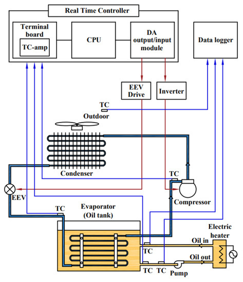
Figure 6.
Schematic of the experimental system.
Table 2.
Specifications of the test unit.
Table 3.
Specifications of the attached devices and oil.
The variable speed compressor is a rotary-type device driven by a three-phase squirrel induction motor. The rotation speed of the variable speed compressor is controlled by a type inverter. The opening angle of the EEV is controlled by adjusting the number of pulses commanded from the EEV drive to the stepping motor mounted inside the EEV. The control system of the MATLAB/Simulink-based real-time controller (RTC) calculates the control input from the set values of and and the state values estimated through the state observer. The calculated control input is converted to an analog voltage reference through the D/A converter in the RTC, and is input to the inverter and EEV drive. In the experiment, the heat load generated during the machining process of the machine tool is applied using an electric heater device.
In the simulations and experiments, the control performances of and , such as command following and control robustness, are analyzed by changing the set values and imposing the heat load to the OCS. The set value of is abruptly changed from °C to °C at 1000 s. The set value of is kept constant at °C, which can be easily controlled while maintaining the maximum COP, selected based on the results of the static characteristic experiments analyzing the relationship between and COP [1,29]. In terms of the heat load variation, 10% of the rated heat load (1.68 kW) is increased at 4000 s, and subsequently, 10% of the rated heat load is decreased again at 6000 s. The sampling time is set as 1 s, considering the dynamic characteristics of the OCS.
Figure 7 and Figure 8 show the simulation and experimental results of the proposed SMC, respectively, when the set value is changed and heat load is imposed. Subfigures (a) show the responses of and . Subfigures (b) and (c) show the responses for and , which are the control inputs of and , respectively. The results indicate that the control responses obtained in the simulation and experiment are highly consistent, demonstrating the suitable design of the SMC.
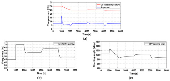
Figure 7.
Simulation results with the SMC. (a) Responses of and . (b) Reference of inverter frequency. (c) Reference of EEV opening angle.
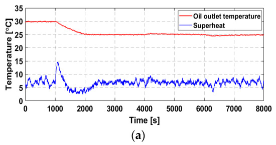
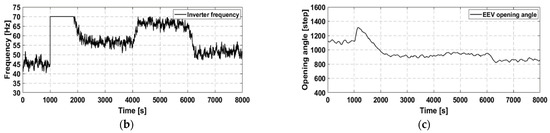
Figure 8.
Experimental results with the SMC. (a) Responses of and (b) Reference of inverter frequency. (c) Reference of EEV opening angle.
In the simulation results shown in Figure 7, the responses of and strictly converge to the target value without a steady-state error, even when the set value is varied and heat load is imposed. These findings indicate the appropriateness of the GA-based SMC optimization based on the satisfaction of the settling time s and undershoot °C, which are transient characteristics when changing the reference. However, the response of exhibits rough transient characteristics with a large overshoot due to the influence of the interference caused by a sudden change in the rotational speed of the compressor when the set value is changed.
Notably, the experimental results shown in Figure 8 are obtained in an environment in which the fluctuations in the heat load and ambient temperature of the experimental devices are different from those during modeling. Therefore, the proposed SMC exhibits a robust control performance despite the model uncertainties and disturbances. In particular, the feedforward controller ensures the prompt convergence of to the target temperature of °C without a steady-state error, even when disturbances caused by heat load fluctuations are applied. In addition, the main controlled variable is strictly controlled within the allowable error range °C, even when the set value is changed and heat load is imposed. These findings demonstrate that the proposed SMC is robust against model uncertainties and disturbances.
Figure 9 shows the experimental results of and based on the proposed SMC under the same conditions as those adopted for Figure 8, except for the ambient temperature of the experimental apparatus.
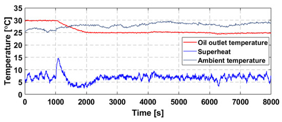
Figure 9.
Responses of and according to the change in the ambient temperature based on SMC.
In the experiment, for 8000 s, the ambient temperature fluctuates irregularly from °C to °C. When the ambient temperature of the experimental device is different from when the nominal model is acquired, the dynamic characteristics of the control object are changed, leading to model uncertainty [1]. As shown in Figure 9, the SMC ensures that converges within the allowable error range °C and follows Ts to the target temperature of °C, despite the model uncertainty.
3.2. Behavior Analysis of State Variables in the Phase Plane
Figure 10a, b show the two-dimensional phase plane obtained from the simulation result shown in Figure 7.
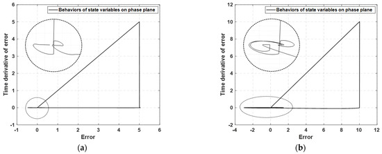
Figure 10.
Behaviors of state variables on the phase plane. (a) Behaviors of and for controlling (b) Behaviors of and for controlling .
To strictly analyze the behaviors of state variables, the region near the origin is enlarged inside the circle. It can be noted that and its derivative converge to the origin (0,0) of the phase plane, even when the set value is changed and heat load is imposed. The designed two-dimensional phase plane can render the behavior of state variables intuitively understandable. This analysis can provide guidance to enhance the control performance of the SMC. If a saturation function is used for , the transient characteristics of deteriorate due to . To prevent chattering and obtain a satisfactory transient response of , it is necessary to appropriately select .
Figure 11 and Figure 12 show the simulation results of applying the signum function and saturation function to , respectively.
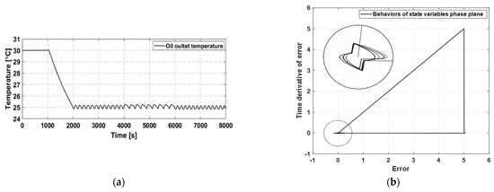
Figure 11.
Simulation results based on a signum function. (a) Response of . (b) Behaviors of and on the phase plane.
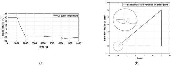
Figure 12.
Simulation results based on a saturation function. (a) Response of . (b) Behaviors of and on the phase plane.
Subfigures (a) show the response of , and subfigures (b) show the behaviors of and . As shown in Figure 11a, rapidly converges to the set value, but chattering occurs. This phenomenon can be clearly observed by analyzing the behaviors of and on the phase plane—the values fluctuate near the origin due to the signum function in Figure 11b. In contrast, Figure 12a shows that chattering can be suppressed by applying the saturation function in the response of . This phenomenon can be clearly observed in Figure 12b in terms of the convergence of and to the origin due to the saturation function. In particular, the saturation function is defined as in the range of . As the of the saturation function increases, in Equation (13) decreases. Consequently, the response of leads to a deterioration in the transient response, such as an increase in the settling time. Therefore, the oil outlet temperature is promptly controlled without chattering within the allowable error range of °C through the optimization of of the saturation function in this study.
3.3. Performance of the Disturbance Estimation Based on the Kalman State Observer
Figure 13 shows the block diagram for the simulation, indicating the position of the disturbance addition and the method of estimating the disturbance. Figure 14 shows the simulation results for the comparison of the applied disturbance (red) and the estimated disturbance (blue) . The disturbance estimation is valid because the added disturbance and estimated disturbance exhibit a reasonable agreement.
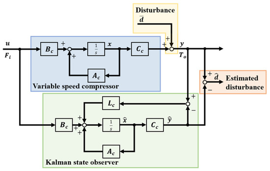
Figure 13.
Disturbance estimation by the Kalman state observer.
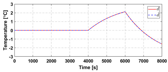
Figure 14.
Comparison between and by simulation.
3.4. Comparison of the Control Performance with a PI Controller
To validate the control performance of the proposed SMC, simulations and experiments based on a PI controller are conducted, and the responses are compared and analyzed. The simulations and experiments are conducted under the same conditions as those for the SMC pertaining to Figure 7 and Figure 8, and the responses of and to changes in the set value and abrupt changes in the heat load are analyzed.
The PI controller is designed using a MATLAB tuner based on the transfer function model indicated in Equation (1). The PI gain for controlling is designed to have the same command-following performance as that of the SMC. Specifically, the settling time is within 1700 s, and the maximum undershoot is °C. The PI gain for controlling is designed by finetuning, similarly to the transient response of the SMC when the set value is changed. In particular, an anti-windup controller is added to the PI controller to prevent the saturation of the manipulated variable due to integral accumulation. Table 4 summarizes the designed PI controller and anti-windup gain for the simulation and experiment.
Table 4.
Designed gains of the PI controller and anti-windup.
Figure 15 and Figure 16 show the results of the simulation and experiment of the PI controller, respectively, when the set value and heat load are changed. Subfigure (a) shows the responses of and . Subfigures (b) and (c), respectively, show the manipulated variables and corresponding to (a). The feasibility of the designed PI controller is confirmed by the agreement between the responses obtained in the simulation and experiment. The slight fluctuations in , as shown in Figure 16a,b, are caused by sensor noise.
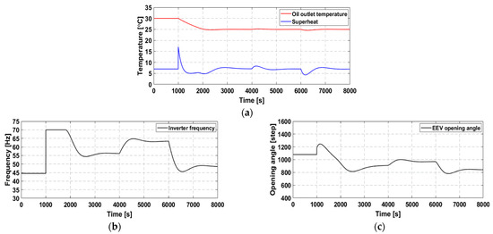
Figure 15.
Simulation results with the PI controller. (a) Responses of and . (b) Reference of inverter frequency. (c) Reference of EEV opening angle.
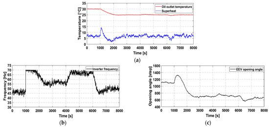
Figure 16.
Experimental results with the PI controller. (a) Responses of and (b) Reference of inverter frequency. (c) Reference of EEV opening angle.
The comparison of the simulation results shown in Figure 7 and Figure 15 indicates that the SMC and PI controllers converge to the target value without a steady-state error, even when the set value and heat load are changed. As shown in Figure 7a and Figure 15a, the transient response of when the set value is abruptly changed is consistent with the designer intent. In addition, the response of exhibits a transient characteristic with a large overshoot due to the interference effect caused by a sudden change in the rotational speed of the compressor when the set value is changed.
The comparison of the experimental results shown in Figure 8 and Figure 16 indicates that the SMC and PI controllers converge to the target value without a steady-state error, even when the set value and heat load are changed. To evaluate the robustness of the two controllers against disturbance, the response of to a change in the heat load is quantitatively analyzed. First, as the heat load increases, the settling time pertaining to the SMC and PI controller is 912 s and 1216 s, respectively, and the maximum overshoot is °C and °C, respectively. Next, when the heat load is reduced, the settling times pertaining to the SMC and PI controller are 1372 s and 1587 s, respectively, and the maximum undershoot values are °C and °C, respectively. These results indicate that the transient characteristics of the main controlled variable when the SMC is used are superior to those associated with the PI controller when the heat load varies. Furthermore, the responses of pertaining to the SMC and PI controller are compared and analyzed when the heat load is varied. First, as the heat load increases, the settling times of pertaining to the SMC and PI controller are 114 s and 526 s, respectively. Next, when the heat load is reduced, the settling times of by the SMC and PI controller are 515 s and 887 s, respectively. In other words, the SMC converges to the target temperature more rapidly than the PI controller when the heat load is varied. Therefore, the control performance of the SMC is more robust than that of the PI controller. Notably, the rigorous quantitative comparative evaluation of the simulation and experimental results based on the SMC and PI controller in this study is performed to highlight the robust control performance of the proposed SMC, rather than to evaluate the relative superiority of the SMC. In particular, when comparing the control performances of the PI and SMC, the control robustness in the case of heat load variations is intensively analyzed after ensuring that the command-following performance is the same.
The control robustness of the SMC for the OCS against model uncertainty and disturbance is examined. After designing a PI controller to validate the performance of the proposed controller, simulations and experiments are performed under the same conditions as those adopted for the SMC. The quantitative comparison and analysis of the robustness of the two controllers demonstrates that the proposed SMC is more robust to disturbances and model uncertainties than the PI controller.
4. Conclusions
An SMC with a two-dimensional phase plane for a VSRS was designed based on a practical state-space model to ensure a robust control performance. In addition, a Kalman state observer was applied for state estimation. A feedforward controller was designed to compensate for the deterioration in the transient response due to the use of the saturation function. The GA was utilized for the design parameter optimization of the saturation function without a cumbersome trial and error process. The proposed controller was validated through simulations and experiments with a VSRS-based OCS. Furthermore, the effectiveness of the proposed method was confirmed by comparing its control performance with that of a conventional PI controller. The key conclusions can be summarized as follows:
- (1)
- The proposed sliding mode controller with a Kalman state observer and feedforward controller exhibits a robust control performance by strictly controlling the target temperature within the allowable steady-state error range of ±0.1 °C, even in the presence of model uncertainty and disturbance;
- (2)
- The optimization of the design parameters of the saturation function with the GA helped enhance the optimal control performance by reducing the chattering and vulnerability of the SMC and eliminating the tediousness of repeated trials;
- (3)
- The use of a low-dimensional state-space nominal model transformed from a practical transfer function obtained through dynamic experiments can facilitate the controller design and reduce model uncertainty, thereby ensuring a robust control performance;
- (4)
- The proposed SMC with a two-dimensional sliding surface can enhance the control performance by facilitating the analysis of the behavior of the state variables in the phase plane.
Author Contributions
Data curation, J.L.; Formal analysis, J.L.; Supervision, S.J.; Writing—original draft, J.L.; Writing—review & editing, S.J. All authors have read and agreed to the published version of the manuscript.
Funding
This work was supported by the “Human Resources Program in Energy Technology” of the Korea Institute of Energy Technology Evaluation and Planning (KETEP), granted financial resource from the Ministry of Trade, Industry and Energy, Republic of Korea. (No. 20184010201700).
Institutional Review Board Statement
Not applicable.
Informed Consent Statement
Not applicable.
Data Availability Statement
Not applicable.
Conflicts of Interest
The authors declare no conflict of interest.
Nomenclature
| coefficient matrix | |
| dead time (s) | |
| control error (°C) | |
| gain of feedforward controller | |
| reference of inverter frequency (Hz) | |
| gain of PI controller | |
| switching gain | |
| DC gain | |
| gain of Kalman filter | |
| state variable in phase plane | |
| controlled variable (°C) | |
| continuous control input (V) | |
| discontinuous control input (V) | |
| feedforward control input (V) | |
| reference of EEV opening angle (step) | |
| variation | |
| gradient of sliding line | |
| sliding function | |
| time constant (s) | |
| measurement noise | |
| process noise | |
| Subscript & Superscript | |
| compressor | |
| EEV | |
| interference effect | |
| oil outlet | |
| superheat | |
| ′ | transpose of matrix |
| estimated value | |
| set value | |
References
- Kim, J.G.; Han, C.H.; Jeong, S.K. Disturbance observer-based robust control against model uncertainty and disturbance for a variable speed refrigeration system. Int. J. Refrig. 2020, 116, 49–59. [Google Scholar] [CrossRef]
- Jeong, S.K.; Lee, D.B.; Hong, K.H. Comparison of System Performance on Hot-gas Bypass and Variable Speed Compressor in an Oil Cooler for Machine Tools. J. Mech. Sci. Technol. 2014, 28, 721–727. [Google Scholar] [CrossRef]
- Jeong, S.K. Optimum robust control for an oil cooler system with variable speed drive of machine tools. J. Korean Soc. Power Syst. Eng. 2019, 23, 18–26. [Google Scholar] [CrossRef]
- Li, H.; Jeong, S.K.; You, S.S. Feedforward control of capacity and superheat for a variable speed refrigeration system. Appl. Therm. Eng. 2009, 29, 1067–1074. [Google Scholar] [CrossRef]
- Li, H.; Jeong, S.K.; Yoon, J.I.; You, S.S. An empirical model for independent control of variable speed refrigeration system. Appl. Therm. Eng. 2008, 28, 1918–1924. [Google Scholar] [CrossRef]
- Jeong, S.K.; Han, C.H.; Li, H.; Wahyu, K.W. Systematic design of membership functions for fuzzy logic control of variable speed refrigeration system. Appl. Therm. Eng. 2018, 142, 303–310. [Google Scholar] [CrossRef]
- Cao, J.P.; Jeong, S.K.; Jung, Y.M. Fuzzy logic controller design with unevenly distributed membership function for high performance chamber cooling system. J. Cent. South Univ. 2014, 21, 2684–2692. [Google Scholar] [CrossRef]
- Quansheng, Z.; Canova, M. Modeling and output feedback control of automotive air conditioning system. Int. J. Refrig. 2015, 58, 207–218. [Google Scholar] [CrossRef]
- Yang, Y.; Wu, M.D.; Chang, Y.C. Temperature control of the four-zone split inverter air conditioners using LMI expression based on LQR for mixed H2/H∞. Appl. Energy 2014, 113, 912–923. [Google Scholar] [CrossRef]
- Schurt, L.C.; Hermes, C.J.; Neto, A.T. A model-driven multivariable controller for vapor compression refrigeration systems. Int. J. Refrig. 2009, 32, 1672–1682. [Google Scholar] [CrossRef]
- Aprea, C.; Mastrullo, R.; Renno, C. Fuzzy control of the compressor speed in a refrigeration plant. Int. J. Refrig. 2004, 27, 639–648. [Google Scholar] [CrossRef]
- Willatzen, M.; Pettit, N.B.O.L.; Ploug-Sorensen, L. A general dynamic simulation model for evaporators and condensers in refrigeration. Part I: Moving-boundary formulation of two-phase flows with heat exchange. Int. J. Refrig. 1998, 21, 398–403. [Google Scholar] [CrossRef]
- Alfonso, D.; Gianluca, L.; Ignazio, M.; Alessandro, P. Second-Order Sliding-Mode Control of DC Drives. IEEE Trans. Ind. Electron. 2004, 51, 364–373. [Google Scholar] [CrossRef]
- Utkin, V.I. Sliding Mode Control Design Principles and Applications to Electric Drives. IEEE Trans. Ind. Electron. 1993, 40, 23–26. [Google Scholar] [CrossRef]
- Utkin, V.I. Variable structure systems with sliding modes. IEEE Trans. Autom. Control 1977, 22, 212–222. [Google Scholar] [CrossRef]
- Lee, S.D.; Lee, B.K.; You, S.S. Sliding Mode Control with Super-Twisting Algorithm for Surge Oscillation of Mooring Vessel System. J. Korean Soc. Mar. Environ. Saf. 2018, 24, 953–959. [Google Scholar] [CrossRef]
- Kim, N.H.; Park, Y.K.; Sun, J.E.; Shin, S.J.; Min, B.H.; Park, H.J.; Kang, S.H.; Hur, H.; Ha, M.Y.; Lee, M.C. Robust sliding mode control of a vapor compression cycle. Int. J. Control Autom. Syst. 2018, 16, 62–78. [Google Scholar] [CrossRef]
- Shah, A.; Huang, D.; Huang, T.; Farid, U. Optimization of BuildingsEnergy Consumption by Designing Sliding Mode Control for Multizone VAV Air Conditioning Systems. Energies 2018, 11, 2911. [Google Scholar] [CrossRef]
- Huang, Y.; Khajepour, A.; Ding, H.; Bagheri, F.; Bahrami, M. An energy-saving set-point optimizer with a sliding mode controller for automotive air-conditioning/refrigeration systems. Appl. Energy 2017, 188, 576–585. [Google Scholar] [CrossRef]
- Kessal, A.; Rahmani, L. Ga-Optimized Parameters of Sliding-Mode Controller Based on Both Output voltage and Input Current with an Application in the PFC of AC/DC Converters. IEEE Trans. Power Electron. 2014, 29, 3159–3165. [Google Scholar] [CrossRef]
- Navale, R.L.; Nelson, R.M. Use of genetic algorithms and evolutionary strategies to develop an adaptive fuzzy logic controller for a cooling coil-Comparison of the AFLC with a standard PID controller. Energy Build. 2012, 45, 169–180. [Google Scholar] [CrossRef]
- Huang, W.; Lam, H.N. Using genetic algorithms to optimize controller parameters for HVAC systems. Energy Build. 1997, 26, 277–282. [Google Scholar] [CrossRef]
- Goldberg, D.E.; Holland, J.H. Genetic Algorithms and Machine Learning. Mach. Learn. 1988, 3, 95–99. [Google Scholar] [CrossRef]
- Rawlins, G.J.E. Foundations of Genetic Algorithms; Elsevier: Amsterdam, The Netherlands, 1991; Volume 1, pp. 1–341. [Google Scholar] [CrossRef]
- Kalman, R.E.; Bucy, R.S. New Results in Linear Filtering and Prediction Theory. J. Basic Eng. 1961, 83, 95–108. [Google Scholar] [CrossRef]
- Kalman, R.E. A New Approach to Linear Filtering and Prediction Problems. J. Basic Eng. 1960, 82, 35–45. [Google Scholar] [CrossRef]
- Luenberger, D. An introduction to observers. IEEE Trans. Autom. Control 1971, 16, 596–602. [Google Scholar] [CrossRef]
- Jung, Y.M.; Jeong, S.K.; Yang, J.H. PI Controller Design of the Refrigeration System Based on Dynamic Characteristic of the Second Order Model. J. Korea Soc. Power Syst. Eng. 2014, 18, 200–206. [Google Scholar] [CrossRef][Green Version]
- Lin, J.L.; Yeh, T.J. Modeling identification and control of air-conditioning systems. Int. J. Refrig. 2007, 30, 202–220. [Google Scholar] [CrossRef]


Publisher’s Note: MDPI stays neutral with regard to jurisdictional claims in published maps and institutional affiliations. |
© 2021 by the authors. Licensee MDPI, Basel, Switzerland. This article is an open access article distributed under the terms and conditions of the Creative Commons Attribution (CC BY) license (https://creativecommons.org/licenses/by/4.0/).