Abstract
Faults in distribution networks can result in severe transients, equipment failure, and power outages. The quick and accurate detection of the faulty section enables the operator to avoid prolonged power outages and economic losses by quickly retrieving the network. However, the occurrence of diverse fault types with various resistances and locations and the highly non-linear nature of distribution networks make fault section detection challenging for numerous conventional techniques. This study presents a cutting-edge deep learning-based algorithm to distinguish fault sections in distribution networks to address these issues. The proposed gated recurrent unit model utilizes only two samples of the angle between the voltage and current on either side of the feeders, which record by smart feeder meters, to detect faulty sections in real time. When a network fault occurs, the protection relays trigger the trip command for the breakers. Immediately, the angle data are obtained from all smart feeder meters of the network, which comprises a pre-fault sample and a post-fault sample. The data are then employed as an input to the pre-trained gated recurrent unit model to determine the faulted line. The performance of this novel algorithm was validated through simulations of various fault types in the IEEE-33 bus system. The model recognizes the faulty section with competitive performance in terms of accuracy.
1. Introduction
Distribution networks, which are responsible for delivering electricity to consumers, are essential parts of the electrical logistics chain. A resilient and stable distribution network should transfer electrical energy to local light manufacturers, residential and commercial customers with minor fluctuation and interruption [1]. However, unwanted events such as equipment malfunction, unauthorized involvements (e.g., human disruptions), and extreme weather conditions may lead the system to experience a fault and, as a result, a shutdown. Hence, various faults with diverse resistances and situations may happen in the distribution networks at numerous locations [2]. Line characteristics can change over time and under different fault conditions, adversely affect fault location procedures and result in erroneous results. On the other hand, financial losses and consumer discontent will ensue if network recovery takes a substantial amount of time owing to incorrect fault location results. Therefore, it is crucial to detect faults promptly and correctly, regardless of their severity and line parameter variation [3]. There is a wide variety of fault location methodologies, each with its own set of advantages. The most well-known fault location strategies include Machine Learning (ML) techniques [4], impedance-based methods [5], traveling wave-based algorithms [6], and state estimation-based approaches [7]. The authors of Ref. [8] provide a comprehensive review of the various types of fault location methods and their associated benefits and drawbacks.
In impedance-based methods, low-resolution recorded data at the network’s substation are employed to locate fault points [9]. The primary drawback of impedance-based strategies is that they cannot recognize the actual faulty section, requiring an additional technique to distinguish the actual fault spot from the other candidates [10]. The authors of Ref. [11] represent a fault location approach for locating the fault spot in a smart distribution network. To improve accuracy, the distributed line model is used. However, the line parameters vary in real-world applications, owing to age and weather conditions. One of the main limitations of this approach is that it requires exact line parameters to perform correctly and accurately. A further disadvantage of impedance-based fault location techniques is that they require the precise load value of each node to function efficiently, which can be alleviated by deploying smart meters in all nodes. In [12], the collected fault data of smart meters and Smart Feeder Meters (SFMs) have been used to pinpoint the specific spot of the fault in a multi-branch distributed network. To cover complete sections of the network, SFMs must be installed in all branches. An impedance-based approach is utilized to discover probable fault spots, and, then, the genuine faulty section is identified using the active power recorded by the SFM. One unpleasant aspect of this approach is that it is reliant on the fault current. In vast distribution networks, this technique is unable to distinguish high impedance fault points accurately. The authors of Ref. [13] resolve the multi-response issue associated with impedance-based techniques by using the frequency component analysis methodology. An innovative impedance-based prevention technique for active distribution networks operating both in islanded and grid-connected modes is suggested in [14]. The recorded data of protection relays and the measurements, which are located at the end of each line, have been used in this methodology. A fault identification index is then defined as a function of a pre-determined constant value and the fault’s equivalent impedance. If the index is larger than the predetermined constant value, the protection functions of relays are executed. The key concern of this technique would be that it lacks a mechanism for locating faulty sections and is susceptible to load uncertainties due to the use of a constant comparative factor in the construction of the fault detection index. To locate the location of the fault in distribution networks, Ref. [15] proposes a novel impedance-based fault localization approach. The modal transformation matrix is employed in this method to mitigate the inherent influence of line parameters on each phase, which creates a dependency in phase formulation. The voltage and current of fault data recorded by the one-end feeding substation are utilized to locate the fault. Although this method is immune to load variation, different fault resistances, time-varying loads, and an unbalanced network operation, it requires precise line parameters for proper functionality. It may acquire multiple fault point nominates utilizing an extra method to specify the real faulty point.
Traveling wave techniques are among the most widely used methods for locating fault points independent of line characteristics [16]. The authors of Ref. [17] present a robust traveling wave-based fault location approach for determining the location of the fault in multi-branch networks. The majority of traveling wave-based techniques include arrival time inaccuracies, which might imperil the entire fault location operation. In this paper, a novel optimization-based technique for mitigating the negative impact of arrival time inaccuracy is given. The particle swarm optimization approach is implemented to reduce the run time and improve precision. The primary drawback of this approach is that it necessitates high sampling rate devices, which are not cost-effective for distribution networks. The authors of [18] offer a new fault locating approach that uses a deviating decomposition mode and an energy analysis of the recorded fault signal to locate the fault spot. Before developing a fault, an intrinsic range variation matrix is generated based on the traveling wave propagation characteristics and the distribution system structure. The fault distance difference matrix is built utilizing all double-ended measurements of the network arrival time of the traveling wave of all records. Finally, the fault distance can be calculated by comparing the two previously described matrices. This technique is not resistant to fault signal arrival time error. Traditional traveling wave fault location approaches only examine time or frequency characteristics, resulting in an incorrect response. The authors of Ref. [19] propose a novel traveling wave time–frequency approach that overcomes the shortcomings of existing methods. First, the arrival time of signals to nodes is identified using a quadratic B-spline wavelet analysis modulus maximum detection technique with a denoising factor. The appropriate velocity of the incident wave is then calculated employing the matrix pencil technique, as well as the frequency of the traveling wave when it arrives at the nodes. Finally, the fault location can be calculated using pre-determined equations and the obtained data of the fault signal.
On active distribution networks with adequate data, state estimation-based fault location methods are primarily employed. In [20], a new state estimation-based fault location approach for active distribution networks is proposed. This work consists of two steps: identifying and locating the fault. First of all, a framework is constructed to distinguish network faults by utilizing the network’s line characteristics, the Jacobian matrix of each section, and the state estimation paradigm. If the output of the least-squares-error-based function is more significant than a pre-determined residual, the problem can be recognized. Then, as a floating node, a new node is defined. Finally, several iterative computations are used to identify the location of the floating point, which is the fault spot. The authors of [21] introduce a new state estimation-based scheme for locating a short circuit fault in active distribution networks. The classic state estimate technique is changed in this aspect to be consistent with fault situations. Then, based on the updated state estimation, a fault localization method is provided, which tends to detect the fault’s location after distinguishing the faulty region. Current and voltage data recorded by measurements, as well as pre-fault condition estimate findings, are employed for this purpose, and the proper location of the fault is identified utilizing computed residual measurement indices. The main weakness of the method is that it only applies to short circuit faults. Because of the existence of various branches in the power distribution network, the availability of only voltage and current data at the start of the line, and a lack of access to information at the end of the network line, detecting the faulted segment in the distribution system has become much more imperative. Two approaches were employed in [22] to identify the network’s faulty section and fault position. At the beginning of the line, the fault distance can be determined by calculating the current at the end of each network line. As a result, in this work, it was attempted to practically approximate the current and voltage at the start and end of each distribution system line by placing smart meters in the network’s main branch and also using information derived from the power flow in the network’s standard operation. More power flow is utilized in this approach to compute the voltage drop of the lines and calculate the current and voltage at the network lines’ ends, allowing the faulty section to be located.
Because of their versatility and performance, Machine Learning (ML) algorithms are among the most promising approaches for locating faults in distribution networks [23]. Today, thanks to the development of ML and neural network techniques and their variety of applications, acceptable results have been obtained in predicting and classifying most power system [24] issues such as event classification and location [25], fault detection [26], security assessment [27], state estimation [28], and load forecasting [29]. Building a proper database for training artificial intelligence algorithms is very crucial. The authors of Ref. [30] present an integrated system for fault classification and localization employing a summation wavelet extreme learning machine. This technique functions by incorporating feature extraction into the learning process. The significant advantage of this technique is that no line parameters are required. The type of fault is identified in the first phase of the method, followed by the location. Because of their varying current levels, distributed generations (DGs) may have an unfavorable effect on the fault location method. In a faulty circumstance, distributed generations respond differently depending on their power levels at the fault time. To address this issue, the authors of [31] propose a new deep learning (DL)-based approach for locating faults in distribution networks equipped with distributed generation. For the learning phase, a standard neural network is being explored. The fault identification step is carried out with raw data of a three-phase voltage and current for both faulty and non-faulty data classes. The performance of the approach is investigated in a variety of fault scenarios. This method’s cross-validation accuracy is 99.52% for all sorts of faults. The primary drawback of this approach is that it is incapable of detecting the faulty section.
In this study, a highly accurate method, independent of the distribution network topology and without the demand for line parameters, is developed employing a DL model for detecting faulty sections in real time. Furthermore, the proposed Gated Recurrent Unit (GRU) model requires only two samples of the angle between the voltage and current on either side of the feeders. Employing the GRU model, feature extraction is conducted hierarchically by the model itself and does not require feature engineering. Regardless of the type of fault occurring in the network, such as a three-phase to ground, two-phase to ground, two-phase, and single-phase to ground fault, the proposed framework can determine the faulty section with highly competitive accuracy. The model’s performance has been validated in various error conditions on the IEEE-33 bus system. The salient contributions of this research are itemized as follows.
- A non-iterative and parameter-free model is introduced to detect faulty sections in distribution networks in real time that uses only the angle between the voltage and current on both sides of the feeder.
- The proposed GRU model can recognize the faulty section for various fault types and does not demand fault type information.
- This approach takes advantage of SFMs’ recorded low-resolution data (a sample in each period) compared to its competitors.
- The model’s performance has been validated on the IEEE-33 bus system, and the results confirm excellent accuracy.
The rest of the paper is structured as follows. In the next Section, the proposed methodology to detect faulty sections is presented in four subsections. Section 3 demonstrates the case study and simulation and the performance evaluation of the model. Finally, the conclusion is reached in Section 4.
2. The Proposed Faulted Section Location Methodology
2.1. Database
Disturbances and faults in power grids cause immediate and fast changes in voltages, currents, and angles throughout the system; these changes are usually more pronounced and have higher amplitude fluctuations near the fault location. However, due to the highly nonlinear nature of power networks, especially distribution networks, caused by abundant power electronics equipment and renewable energy sources, short line lengths, and similar fluctuations in voltage and current quantities of lines during faults, the performance of model-based techniques to identify the fault location has almost been associated with various difficulties and challenges, so that many model-based methods are not able to recognize the faulty line with high accuracy. In contrast, data-driven techniques are not dependent on network structure.
One of the variables affected after a fault in distribution networks is the angle between voltage and current on both sides of the fault section. The proposed method employs the angle between voltage and current on both sides of each section to distinguish the fault section in distribution networks. In Figure 1, a 3-phase to the ground fault occurred in the distribution line. When a fault occurs in the distribution network, the relays detect it and trigger the trip signal. Instantly, angles between the voltage and current of all three phases on both sides of the section were collected. Angles were sampled from SFMs with a sampling frequency of 50 Hz, which the data window included a pre-fault and a post-fault sample. Finally, applying Equation (4), the difference of the angle between the voltage and current on both sides of the section was calculated and used as the input variable to the proposed GRU model. How to achieve this variable is represented in Equations (1)–(4).
where ,, , and are voltages of the sender and receiver busbars and their angles, respectively. , , , and are also the currents of the sides of the section and their angles, respectively. a, b, and c also represent phases A, B, and C.
where and are the angles between voltage and current on both sides of the section, respectively, and is the section variable used for the proposed section detection framework. Since the data window contains two samples, the value was calculated for the pre-fault and post-fault samples separately, so, for each section, the matrix contains six elements. Eventually, to determine the exact section where the fault occurred, the values must be calculated for all sections (Equation (4)). For example, for the IEEE-33 bus system, which has 32 sections, the β matrix will have dimensions of . Accordingly, when a fault occurs in the network, a matrix with dimensions will be formed, where n is the number of sections in the network. This matrix is then given as input to the pre-trained GRU model to determine where the fault occurred. The more severe the fault and the more phases involved, the easier it will be to find the faulty section in this algorithm; because the difference in angles in Equation (3) for the faulty line will be accompanied by more variations, it will help the DL model to find that section more easily.
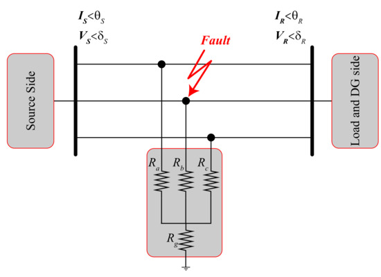
Figure 1.
A three-phase-to-ground fault in a section of a distribution network.
2.2. Recurrent Neural Networks
As one of the most advanced and state-of-the-art ML algorithms, DL has improved the performance of data-driven methods by producing a big hypothesis space. Recurrent Neural Network (RNN) is one of the robust DL algorithms widely utilized to deal with sequences such as time series. The RNN model employs previous information in the sequence to generate the current output using the memory embedded in it, distinguishing RNN from other data-driven approaches.
By increasing the number of hidden layers in a DL model, the model can distinguish more complex functions. The back-propagation algorithm was employed in DL to fine-tune network weights and parameters. In the back-propagation algorithm, for a model with n hidden layers, n derivatives were multiplied by each other. Now, if these derivatives were large, the gradients increased exponentially to the point that they caused an explosion and the model weights tend to be infinite or NAN. In contrast, if the derivatives were small, the gradient decreased exponentially to the point that the gradient disappeared or became zero in deep networks. Vanishing gradient and exploding gradient issues in the back-propagation algorithm can afford slow convergence and significant and undesirable changes in the values of weights, respectively.
RNN method usually encounters vanishing gradient and exploding gradient issues in the back-propagation algorithm. Hence, Long Short-Term Memory (LSTM) and GRU methods, which are subsets of RNN, were developed to address these problems. These two algorithms use internal mechanisms called gates to regulate the flow of information in the network. Gates learn the essential inputs of the sequence and store them in a memory unit. Consequently, they are able to convey information well in long sequences and increase the accuracy of prediction and classification.
2.2.1. LSTM Model
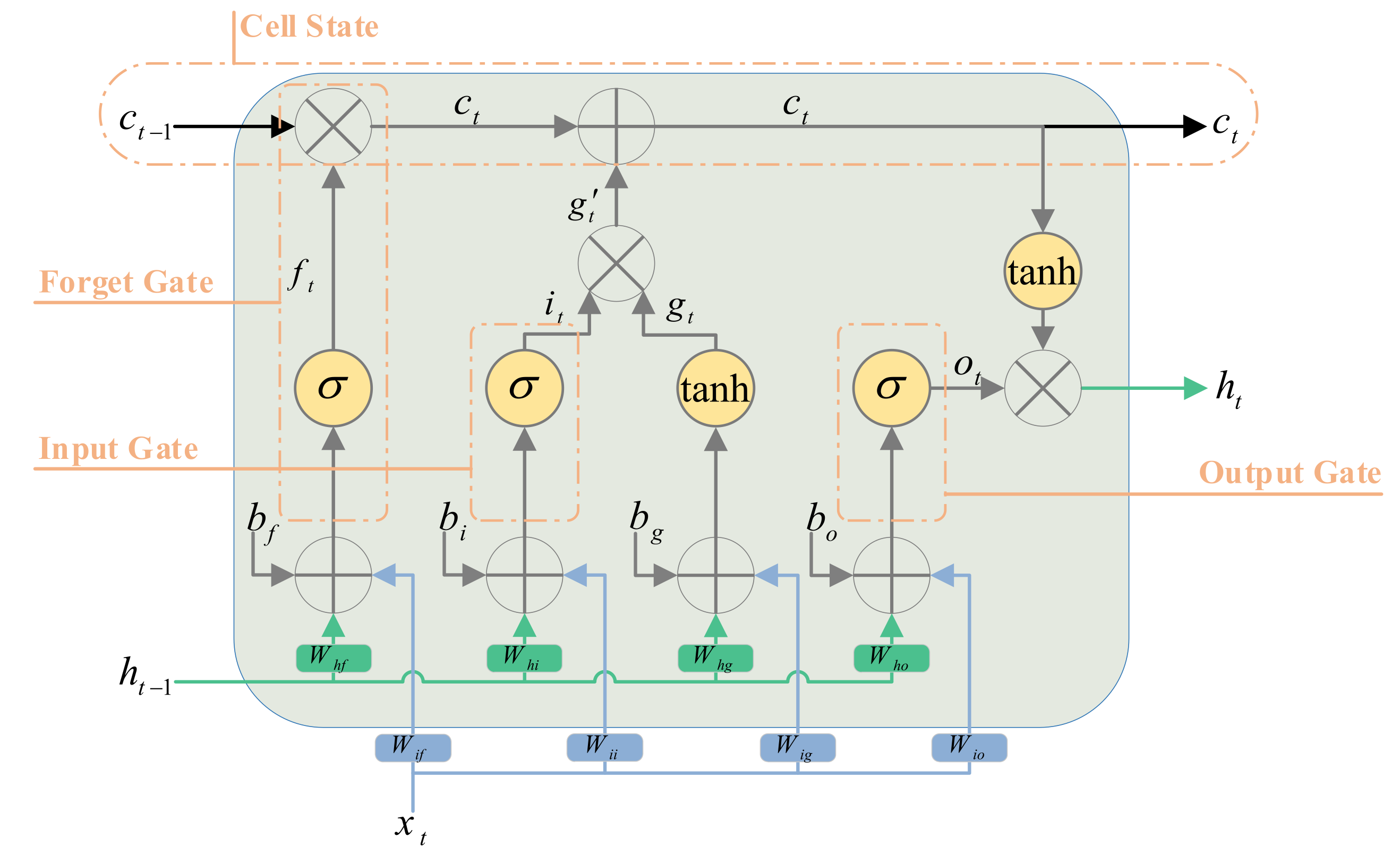
Cell state is the core concept behind the LSTM, also known as the long-term memory unit. The cell state () updates in every step of the sequence according to input to create a temporal feature vector . LSTM regulates the flow of information through three gates called forget gate (), input gate (), and output gate (). Forget gate decides what information should be removed or kept. Forget gate value is a number between 0 and 1; if this value is closer to 0, it means forgetting, and if it is closer to 1, it means keeping information. The sigmoid activation function () does this. The input gate determines new information additions from the current time step and then updated the cell state by . Eventually, the output gate specifies the extent of the previous step information carried over to the subsequent step, including the current time step information. The LSTM equations were as follows:
where and are weights and biases values of the LSTM in every gate. The LSTM structure is presented in Figure 2.
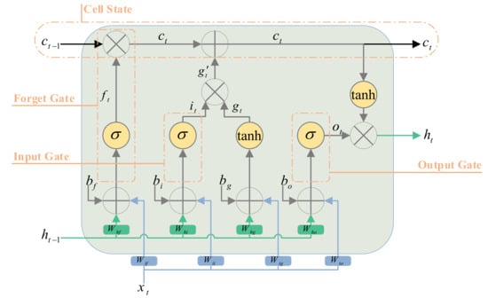
Figure 2.
Illustration of LSTM structure.
2.2.2. GRU Model
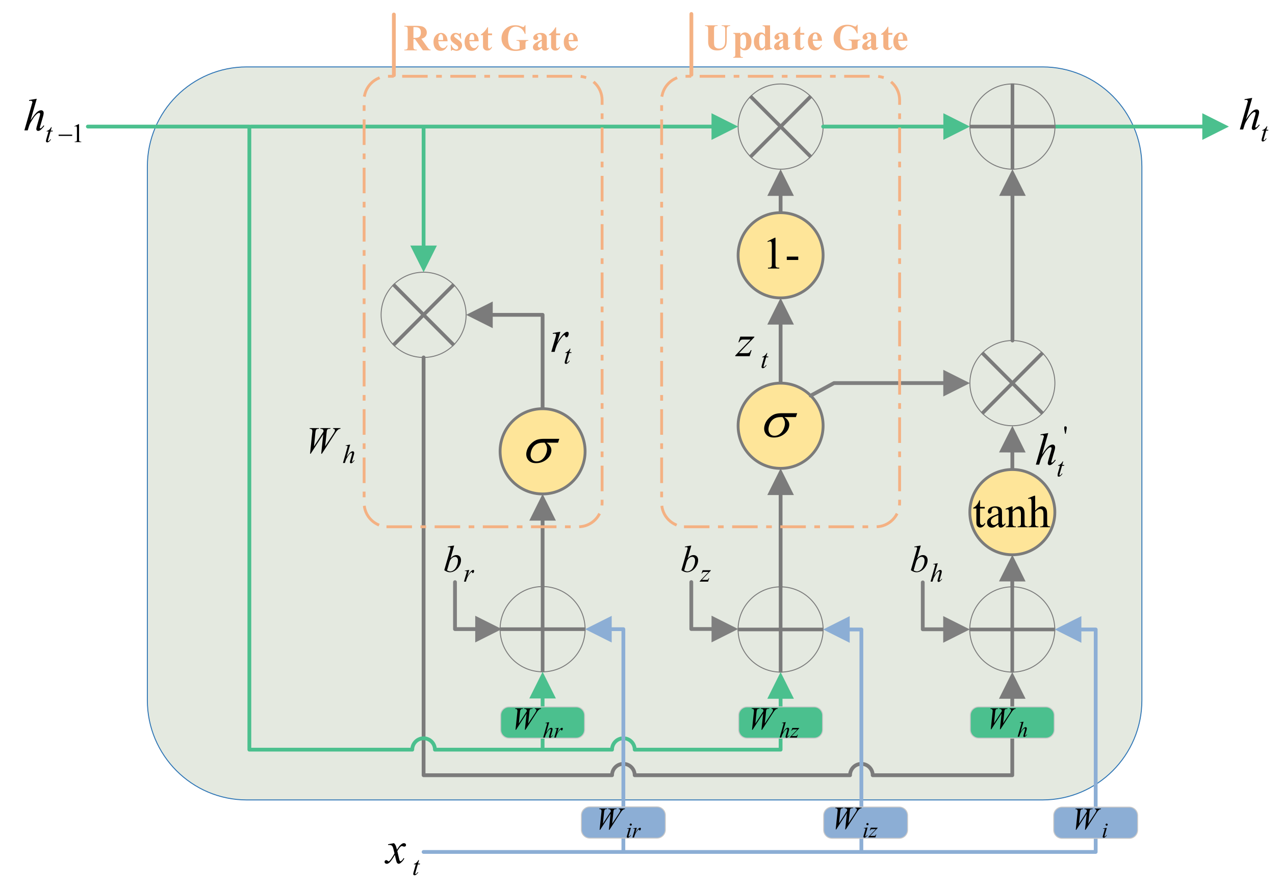
GRU is a simpler type of LSTM consisting of only two gates, Update and Reset, which reduce the number of parameters of the model compared to LSTM. Dissimilar to LSTM, which employs the cell state to store and transfer information, GRU utilizes the hidden state (). The update gate () has a similar function to both forget and input gates in the LSTM model. Additionally, the reset gate () determines how much past information is not required in the current step and should be forgotten. The GRU model was defined by Equations (11)–(14) [32].
where and are weights and biases values of the GRU. The GRU structure is shown in Figure 3.
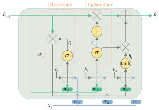
Figure 3.
Illustration of GRU structure.
Due to the comparable performance of GRU and LSTM, employing both models will usually have the same outcomes. However, because the GRU has fewer parameters and is more straightforward to implement than the LSTM, it is faster to train and performs better on small amounts of training data and a lesser data size is required to capture the properties of the data. Consequently, in this study, the same method was utilized to develop the proposed algorithm for determining faulty lines in distribution networks.
2.3. Layers
In the proposed DL model structure, besides the GRU layers, there are other successive layers. These layers comprise the drop-out layer, batch normalization (BN) layer, flatten, dense layer, and softmax layer, which together can develop a DL network. Dense and softmax layers are usually utilized at the end of a structure for classification. Each of these layers is described below:
Drop-out layer: DL networks utilize regularization strategies to avoid overfitting and alleviate the gradient vanishing problem. The most popular and influential of which are dropout [33] and BN [34]. The dropout, which is only applied throughout training, randomly excludes some neurons with probability, which reduces the overfitting issue.
BN layer: In a DL model, since the parameters of each layer change while training, it changes the distribution of input data to the subsequent layers, which reduces the speed of model training. To tackle this issue, BN was introduced, which is a way of accelerating training. This state-of-the-art strategy normalizes each layer’s input data with a mean of 0 and a variance of 1 [34].
Flatten layer: Flatten layer was proposed to reshape the input tensor into a shape (batch dimension, features). For instance, if the layer has an input with dimensions (batch dimension,3,3), by applying the flatten layer, it transforms the tensor to dimensions (batch dimension,9). This layer was utilized before the dense layer.
Dense layer: In a dense layer, all the input neurons are connected to every output by weights. This means that each output is the result of function on all input neurons. This layer is also known as the fully connected layer.
Softmax layer: The softmax mathematical function transforms the input vector to the probability vector. This probability vector estimates the probability that the data relates to a specific class. Thus, softmax has the equivalent function as the sigmoid function; moreover, the sum of all classes’ probabilities are 1. Equation (15) shows the softmax function, where is the input vector to the layer with length [35].
2.4. Architecture of the Proposed GRU Model
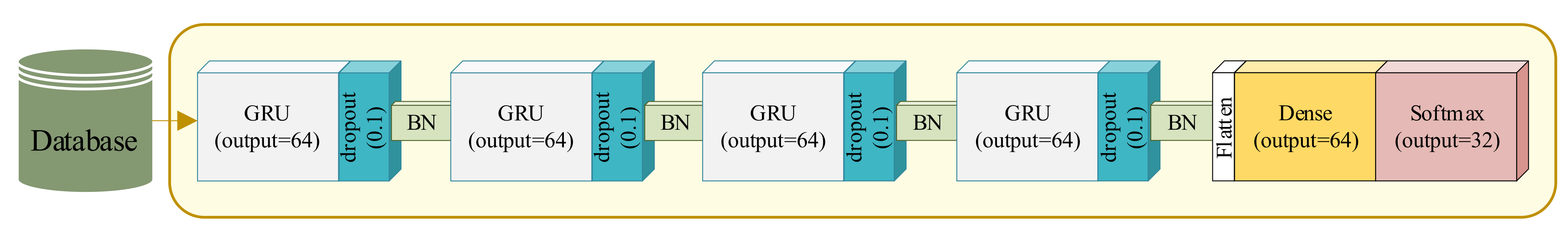
The structure of the proposed GRU model to recognize faulty lines is demonstrated in Figure 4. The proposed model was able to identify faulty sections for various faults, including three-phase to ground fault, two-phase to ground fault, two-phase, and single-phase fault. Four GRU layers were employed in the model, and, following each layer, two regularization strategies (dropout and BN) were used to prevent overfitting. The dropout value for all layers was set to 0.1. The simulation data in DIgSILENT PowerFactory software were applied in various scenarios of faults to create the database. The number of outputs of the softmax layer was equal to the number of classes or, more precisely, the number of sections in the network. For illustration, for the IEEE-33 bus system, there were 32 sections, and the model had to ultimately estimate which section the fault occurred in.

Figure 4.
The architecture of the proposed GRU model.
To tune the models’ parameter and hyperparameters values, an Adam optimizer with learning rate, weight decay, and momentum as 0.001, , and 0.9, respectively, was employed to catch the best and most accurate results. Additionally, the sparse_categorical_crossentropy loss function was chosen in this study.
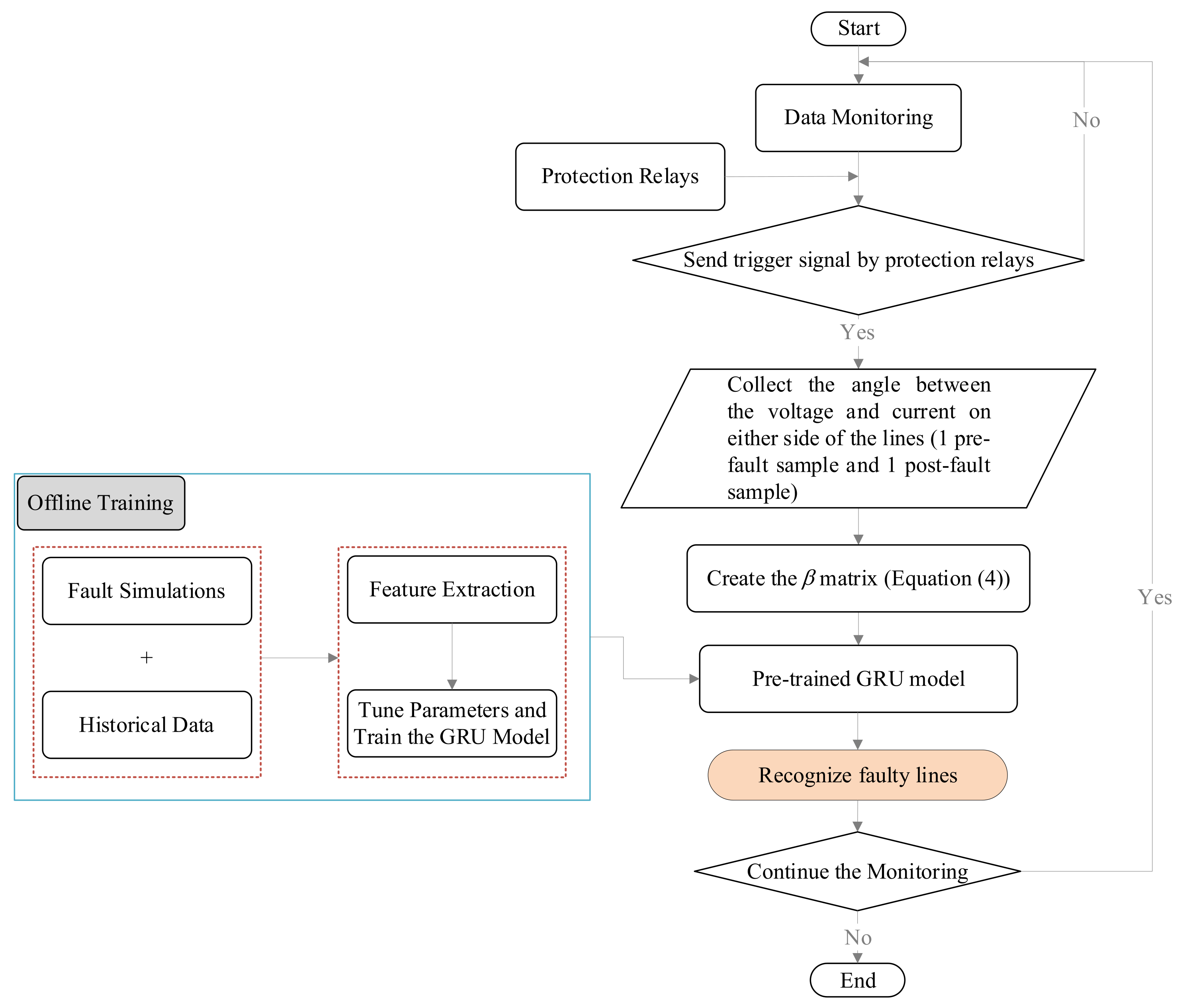
The free parameter proposed model evaluated and detected fault sections in real time. The framework of the proposed method is demonstrated in Figure 5. When a fault occurred in the distribution network, the protection relays issued a trip command and triggered the proposed GRU model. Voltage and current angles were then measured and collected from all SFMs installed on either side of all sections. Each time series of voltage and current angles consisted of two samples, a pre-fault, and a post-fault sample. For all SFMs, the angle between the voltage and current of both samples was calculated. Considering two SFMs were embedded per section, the vector introduced in Equation (3) could be formed. Ultimately, for all sections, the vector was constructed to achieve matrix Equation (4). The matrix was given as input to the pre-trained GRU model to estimate the faulty section.
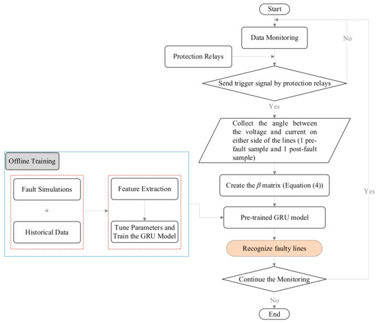
Figure 5.
The proposed framework to recognize the faulty line.
3. Case Study
3.1. Distribution Network without the Presence of DGs
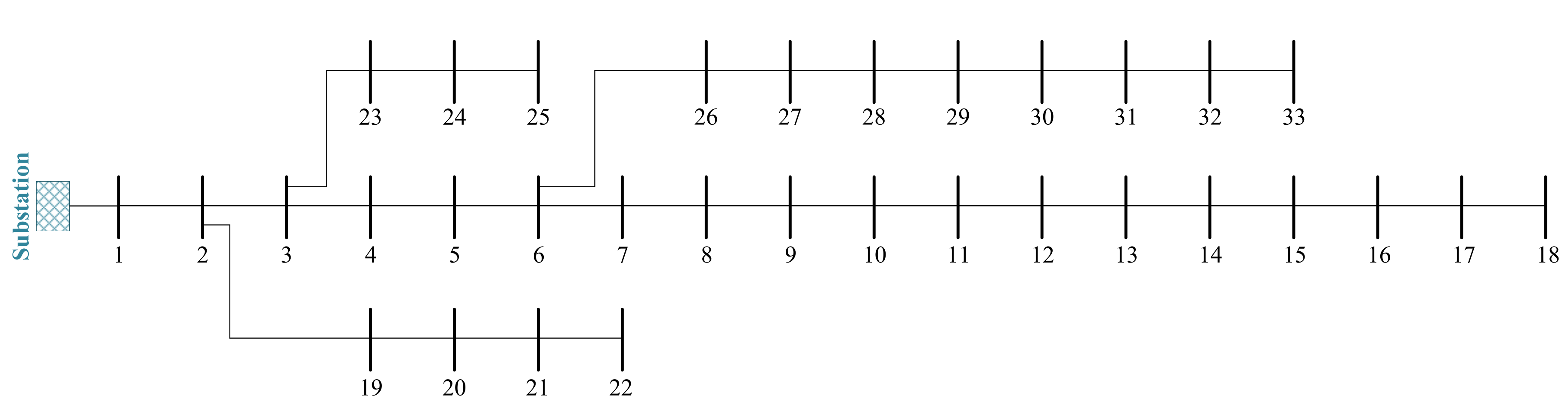
The angle between the voltage and current in each SFM varied according to the fault type, location in the line, fault resistance, and fault inception angle. Hence, various scenarios were simulated in the DIgSILENT PowerFactory software on the IEEE-33 bus system (Figure 6) to generate a proper database. Simulated scenarios are given in Table 1, including a total of 17,280 cases. In all scenarios, a matrix with dimensions of was formed as the matrix. Out of 17,280 scenarios created, 52.5% of the data were utilized for training, 17.5% for validation data, and the rest for testing. The proposed GRU model was trained in Python 3.8.3 on a personal workstation in Python 3.8.3 with 16 GB of RAM and an Intel i7-3820QM CPU working at 2.7 GHz.
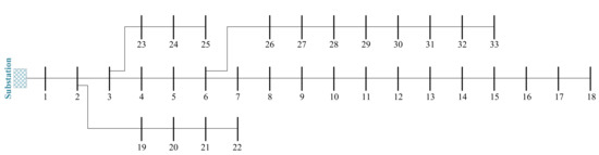
Figure 6.
Single-line diagram of the IEEE-33 bus system.

Table 1.
Proposed method effectiveness under Different fault resistances.
Once the proposed GRU model and its parameters and hyper-parameters fitted, it was vital to assess the model’s performance on the test data. Hence, in this study, the accuracy criterion was utilized. A total of 5184 scenarios were considered for the test set, including three-phase to ground, two-phase to ground, two-phase, and single-phase to ground faults in various circumstances mentioned in Table 1, on all network lines with equal proportions.
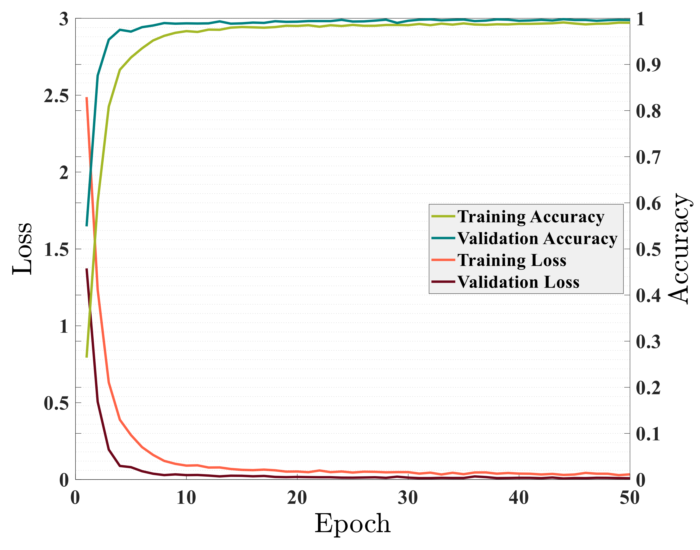
Figure 7 demonstrated the relationship between accuracy and loss on training data and validation data while training the GRU model. As shown in Figure 7, the model was well trained and the training and validation data converge around the 30th epoch. After about epoch 30, the model found its final and desired weight values and parameters, and further training of the model did not help improve the model’s performance. During the training of the model, the running time in each epoch was approximately 25 s. The model’s accuracy on training data became 99.04% during training, and validation data reached 99.64%. In contrast, the training and validation loss tended to be zero. All of this demonstrated the excellent ability of the proposed GRU model to solve the problem of fault section detection in distribution networks. The trained model was, now, applied to predict test data. The accuracy of the proposed model on the test set was 99.56%. Out of 5184 new scenarios given to the model, the fault section in 5161 scenarios was accurately classified.
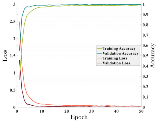
Figure 7.
Accuracy and loss on train and validation sets without DGs penetration in the network.
A confusion matrix could be employed to assess the performance of a classification model on test data more accurately. This matrix had dimensions, in which N is the number of target classes. The matrix compared the actual targets with the targets predicted by the DL and gave an intuitive view that determined how well the proposed classification model had performed. The confusion matrix also specified which classes were not correctly identified by the trained model. Figure 8 demonstrated the confusion matrix for the test data. The proposed model detected most of the fault sections with 100% accuracy. The most misdiagnosis was in Class 8, which, out of 177 scenarios for this class, miscategorized 10 scenarios in Class 7. This very high accuracy is very desirable and competitive for the distribution network, where the length of the lines is very short, and the lines have similar functions at the time of fault conditions. In the “Total” column of Figure 8, the ratio of faulty sections to the total of scenarios correctly detected by the model is shown; the model correctly identified the faulty section related to 5161 scenarios out of 5184 created scenarios. Therefore, the faulty section was detected in 99.56% of the total scenarios.
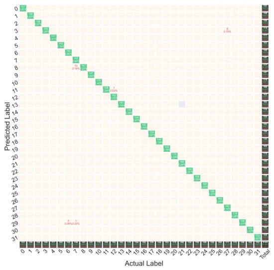
Figure 8.
Confusion matrix for the test data.
The timeline of the proposed model for detecting the faulty section, from the moment the fault occurred to the moment the section was determined, is presented in Figure 9. A pre-fault sample and a post-fault sample were required to distinguish the faulty section. It took 100 milliseconds to delay sending data from SFMs to the data aggregation center. After collecting the data, the proposed GRU model specified the faulty section for the operator in just 55 milliseconds. This figure demonstrated how quickly this algorithm can locate the damaged portion of the network. However, in real-world applications, there is more time to fix the damaged part. On the other hand, this article discusses the issue of fault location and assumes that the fault was completely detected. As a result, the required relays were activated, and the network was cleared of the fault. It was expected in this system that each fault was identified independently and eliminated through relays. As a consequence, the time required to find the fault was 0.56 s, which was different from the time required to detect the fault, and the relays had to respond extremely quickly to prevent possible risks of fault in the network.
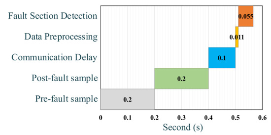
Figure 9.
Fault section detection timeline.
3.2. Distribution Network with the Presence of DGs
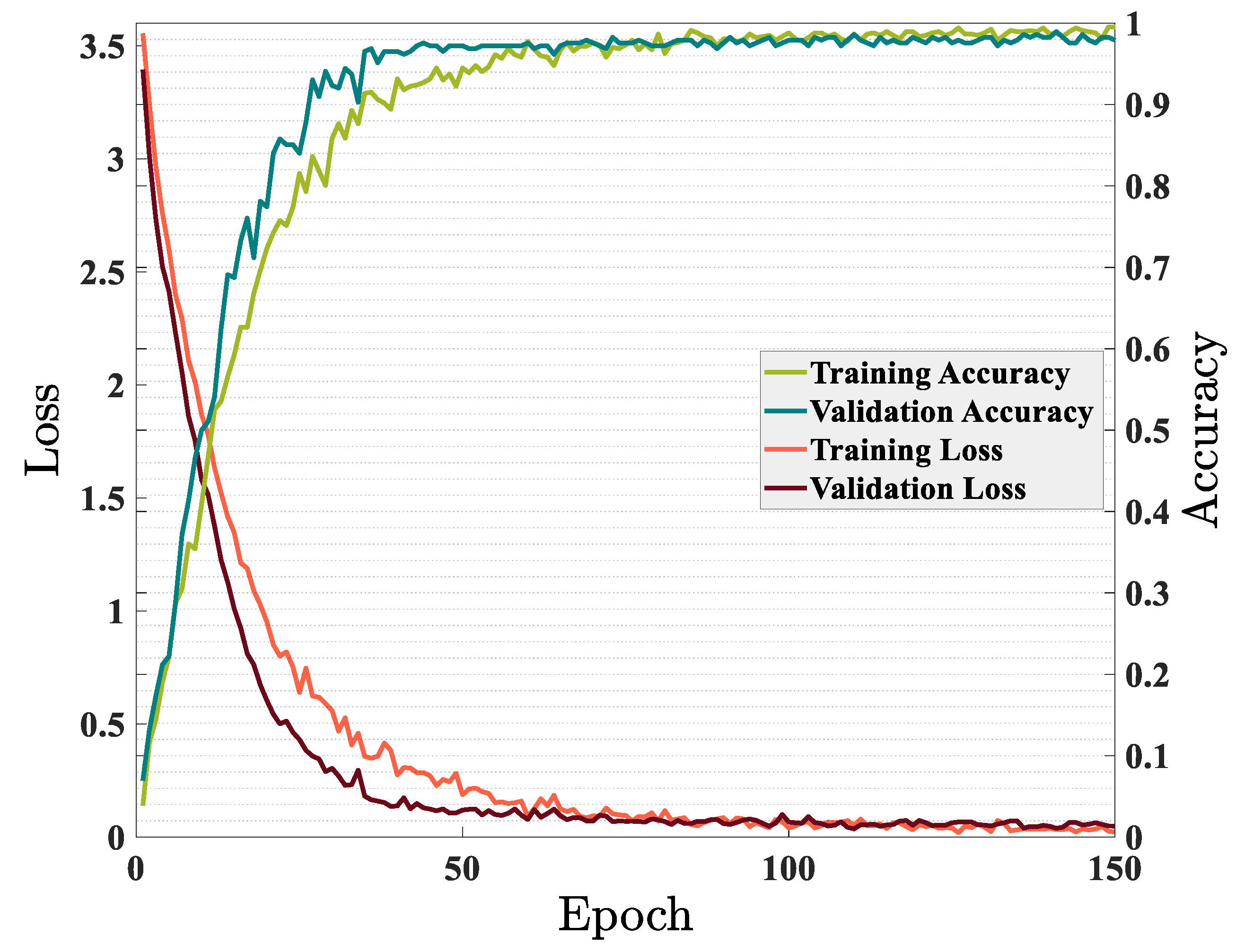
To investigate the impact of DG penetration in the distribution network, five identical DGs with an active generating power of 200 kW and a reactive generating power of 100 kvar were added to the IEEE-33 bus system; DGs were installed in busbars 04, 06, 16, 22, and 31. The scenarios listed in Table 1 were, then, re-generated for this network. After that, the proposed GRU model was trained again with generated data. Figure 10 demonstrates how the proposed GRU model was trained for a distribution network with DGs penetration. As shown in Figure 10, in this case, the GRU model needed more epochs to learn its parameters, and after about 150 epochs, it had almost reached the ideal parameters to find the faulty section, and the amount of loss was minimized. However, the model’s accuracy on training data reached 99.55%, and the accuracy on validation data reached 97.92%.

Figure 10.
Accuracy and loss on train and validation sets with DGs penetration in the network.
4. Conclusions
A real-time and accurate detection of faulty lines in distribution networks is crucial to supply consumers’ demand and prevent long-term power outages and financial losses. This study introduced a cutting-edge method for diagnosing faulty sections in distribution networks utilizing the GRU model that does not require network line impedance parameters. The trained GRU model focused on the angle between the voltage and current of each feeder before and after the fault for the specified purpose. The data window consisted of only two samples obtained with the sampling frequency of 50 Hz from the SFMs installed in the busbars. Since the proposed method was non-iterative, it can be implemented in real time. This state-of-the-art model appeared robust in detecting faulty sections in various fault scenarios, including three-phase to ground, two-phase to ground, two-phase, and single-phase faults with diverse fault inception angles and a variety of resistance, including high impedance faults. The model was validated on the IEEE 33-bus system, and the model reached a very desirable accuracy of 99.56% for the network without DGs penetration and 97.98% with DGs penetration.
Author Contributions
M.R.S.: Conceptualization, Data curation, Formal analysis, Investigation, Methodology, Validation, Writing—original draft. H.M.: Conceptualization, Data curation, Formal analysis, Investigation, Methodology, Validation, Writing—original draft. R.D.: Conceptualization, Funding acquisition, Investigation, Methodology, Project administration, Resources, Supervision, Writing—original draft. M.-T.A.: Conceptualization, Funding acquisition, Investigation, Methodology, Project administration, Resources, Supervision, Writing—original draft. H.R.S.: Conceptualization, Funding acquisition, Project administration, Supervision, Writing—review & editing. All authors have read and agreed to the published version of the manuscript.
Funding
This research received no external funding.
Institutional Review Board Statement
Not applicable.
Informed Consent Statement
Not applicable.
Data Availability Statement
Not applicable.
Conflicts of Interest
The authors declare no conflict of interest.
References
- Mirshekali, H.; Dashti, R.; Shaker, H.R.; Samsami, R.; Torabi, A.J. Linear and Nonlinear Fault Location in Smart Distribution Network under Line Parameter Uncertainty. IEEE Trans. Ind. Inform. 2021. [Google Scholar] [CrossRef]
- Janjic, A.; Velimirovic, L. Integrated fault location and isolation strategy in distribution networks using Markov decision process. Electr. Power Syst. Res. 2020, 180, 106172. [Google Scholar] [CrossRef]
- Lu, D.; Liu, Y.; Chen, S.; Wang, B.; Lu, D. An Improved Noniterative Parameter-Free Fault Location Method on Untransposed Transmission Lines Using Multi-Section Models. IEEE Trans. Power Deliv. 2021. [Google Scholar] [CrossRef]
- Fahim, S.R.; Sarker, S.K.; Muyeen, S.M.; Sheikh, M.R.I.; Das, S.K. Microgrid fault detection and classification: Machine learning based approach, comparison, and reviews. Energies 2020, 13, 3460. [Google Scholar] [CrossRef]
- Mirshekali, H.; Dashti, R.; Shaker, H.R. An Accurate Fault Location Algorithm for Smart Electrical Distribution Systems Equipped with Micro Phasor Mesaurement Units. In Proceedings of the 2019 International Symposium on Advanced Electrical and Communication Technologies, ISAECT 2019, Rome, Italy, 27–29 November 2019. [Google Scholar]
- Shi, Y.; Zheng, T.; Yang, C. Reflected traveling wave based single-ended fault location in distribution networks. Energies 2020, 13, 3917. [Google Scholar] [CrossRef]
- Liu, Y.; Sakis Meliopoulos, A.P.; Tan, Z.; Sun, L.; Fan, R. Dynamic state estimation-based fault locating on transmission lines. IET-Gen. Trans. Dist. 2017, 11, 4184–4192. [Google Scholar] [CrossRef] [Green Version]
- Dashti, R.; Daisy, M.; Mirshekali, H.; Shaker, H.R.; Hosseini Aliabadi, M. A survey of fault prediction and location methods in electrical energy distribution networks. Measurement 2021, 184, 109947. [Google Scholar] [CrossRef]
- Daisy, M.; Dashti, R. Single phase fault location in power distribution network using combination of impedance based method and voltage sage matching algorithm. In Proceedings of the 6th International Conference Modeling Simulation, Applied Optimization ICMSAO 2015—Dedicated to Memory Late Ibrahim El-Sadek, Istanbul, Turkey, 27–29 May 2015. [Google Scholar] [CrossRef]
- Dashti, R.; Sadeh, J. A new method for fault section estimation in distribution network. In Proceedings of the 2010 International Conference on Power System Technology, Hangzhou, China, 24–28 October 2010. [Google Scholar] [CrossRef]
- Mirshekali, H.; Dashti, R.; Keshavarz, A.; Torabi, A.J.; Shaker, H.R. A Novel Fault Location Methodology for Smart Distribution Networks. IEEE Trans. Smart Grid 2020, 12, 1277–1288. [Google Scholar] [CrossRef]
- Mirshekali, H.; Dashti, R.; Handrup, K.; Shaker, H.R. Real fault location in a distribution network using smart feeder meter data. Energies 2021, 14, 3242. [Google Scholar] [CrossRef]
- Gord, E.; Dashti, R.; Najafi, M.; Shaker, H.R. Real Fault Section Estimation in Electrical Distribution Networks Based on the Fault Frequency Component Analysis. Energies 2019, 12, 1145. [Google Scholar] [CrossRef] [Green Version]
- Nobakhti, S.M.; Ketabi, A.; Shafie-Khah, M. A new impedance-based main and backup protection scheme for active distribution lines in ac microgrids. Energies 2021, 14, 274. [Google Scholar] [CrossRef]
- Gabr, M.A.; Ibrahim, D.K.; Ahmed, E.S.; Gilany, M.I. A new impedance-based fault location scheme for overhead unbalanced radial distribution networks. Electr. Power Syst. Res. 2017, 142, 153–162. [Google Scholar] [CrossRef]
- Aftab, M.A.; Hussain, S.M.S.; Ali, I.; Ustun, T.S. Dynamic protection of power systems with high penetration of renewables: A review of the traveling wave based fault location techniques. Int. J. Electr. Power Energy Syst. 2020, 114, 105410. [Google Scholar] [CrossRef]
- Qiao, J.; Yin, X.; Wang, Y.; Xu, W.; Tan, L. A multi-terminal traveling wave fault location method for active distribution network based on residual clustering. Int. J. Electr. Power Energy Syst. 2021, 131, 107070. [Google Scholar] [CrossRef]
- Xie, L.; Luo, L.; Li, Y.; Zhang, Y.; Cao, Y. A Traveling Wave-Based Fault Location Method Employing VMD-TEO for Distribution Network. IEEE Trans. Power Deliv. 2020, 35, 1987–1998. [Google Scholar] [CrossRef]
- Jianwen, Z.; Hui, H.; Yu, G.; Yongping, H.; Shuping, G.; Jianan, L. Single-phase ground fault location method for distribution network based on traveling wave time-frequency characteristics. Electr. Power Syst. Res. 2020, 186, 106401. [Google Scholar] [CrossRef]
- Pignati, M.; Zanni, L.; Romano, P.; Cherkaoui, R.; Paolone, M. Fault Detection and Faulted Line Identification in Active Distribution Networks Using Synchrophasors-Based Real-Time State Estimation. IEEE Trans. Power Deliv. 2017, 32, 381–392. [Google Scholar] [CrossRef] [Green Version]
- Gholami, M.; Abbaspour, A.; Moeini-Aghtaie, M.; Fotuhi-Firuzabad, M.; Lehtonen, M. Detecting the Location of Short-Circuit Faults in Active Distribution Network Using PMU-Based State Estimation. IEEE Trans. Smart Grid 2020, 11, 1396–1406. [Google Scholar] [CrossRef]
- Dashtdar, M.; Sadegh Hosseinimoghadam, S.M.; Dashtdar, M. Fault location in the distribution network based on power system status estimation with smart meters data. Int. J. Emerg. Electr. Power Syst. 2021, 22, 129–147. [Google Scholar]
- Yin, X.; Li, X.; Zhang, Y.; Zhang, T.; Lu, C.; Ai, Q.; Li, Z.; Sun, Z. A Survey of Deep Learning and Its Application in Distribution Network. In Proceedings of the 2020 International Conference on Artificial Intelligence in Information and Communication, ICAIIC 2020, Fukuoka, Japan, 19–21 February; 2020; pp. 643–646. [Google Scholar]
- Khodayar, M.; Liu, G.; Wang, J.; Khodayar, M.E. Deep learning in power systems research: A review. CSEE J. Power Energy Syst. 2021, 7, 209–220. [Google Scholar]
- Shadi, M.R.; Ameli, M.-T.; Azad, S. A real-time hierarchical framework for fault detection, classification, and location in power systems using PMUs data and deep learning. Int. J. Electr. Power Energy Syst. 2021, 134, 107399. [Google Scholar] [CrossRef]
- Helbing, G.; Ritter, M. Deep Learning for fault detection in wind turbines. Renew. Sustain. Energy Rev. 2018, 98, 189–198. [Google Scholar] [CrossRef]
- Sun, M.; Konstantelos, I.; Strbac, G. A Deep Learning-Based Feature Extraction Framework for System Security Assessment. IEEE Trans. Smart Grid 2018. [Google Scholar] [CrossRef]
- Goleijani, S.; Ameli, M.T. Neural network-based power system dynamic state estimation using hybrid data from SCADA and phasor measurement units. Int. Trans. Electr. Energy Syst. 2018, 28, e2481. [Google Scholar] [CrossRef]
- Nahari, A.; Rostami, H.; Dashti, R. Electrical Load Forecasting in Power Distribution Network by Using Artificial Neural Network. Int. J. Electr. Commun. Comp. Eng. 2013, 4, 1737–1743. [Google Scholar]
- Chen, Y.Q.; Fink, O.; Sansavini, G. Combined Fault Location and Classification for Power Transmission Lines Fault Diagnosis With Integrated Feature Extraction. IEEE Trans. Ind. Electron. 2018, 65, 561–569. [Google Scholar] [CrossRef]
- Rai, P.; Londhe, N.D.; Raj, R. Fault classification in power system distribution network integrated with distributed generators using CNN. Electr. Power Syst. Res. 2021, 192, 106914. [Google Scholar] [CrossRef]
- Chung, J.; Gulcehre, C.; Cho, K.; Bengio, Y. Empirical Evaluation of Gated Recurrent Neural Networks on Sequence Modeling. arXiv 2014, arXiv:1412.3555. [Google Scholar]
- Srivastava, N.; Hinton, G.; Krizhevsky, A.; Salakhutdinov, R. Dropout: A Simple Way to Prevent Neural Networks from Overfitting. J. Mach. Learn. Res. 2014, 15, 1929–1958. [Google Scholar]
- Ioffe, S.; Szegedy, C. Batch Normalization: Accelerating Deep Network Training by Reducing Internal Covariate Shift. In Proceedings of the International Conference on Machine Learning, Lille, France, 6–11 July 2015. [Google Scholar]
- Wang, S.; Chen, H. A novel deep learning method for the classification of power quality disturbances using deep convolutional neural network. Appl. Energy 2019, 235, 1126–1140. [Google Scholar] [CrossRef]


Publisher’s Note: MDPI stays neutral with regard to jurisdictional claims in published maps and institutional affiliations. |
© 2021 by the authors. Licensee MDPI, Basel, Switzerland. This article is an open access article distributed under the terms and conditions of the Creative Commons Attribution (CC BY) license (https://creativecommons.org/licenses/by/4.0/).