Techno-Economic Efficiency Analysis of Various Operating Strategies for Micro-Hydro Storage Using a Pump as a Turbine

Abstract

Storage technologies are an increasingly crucial element in the continued expansion of renewable energy production. Micro-hydro storage using a pump as a turbine is a potentially promising solution in certain cases, for example, for extending existing photovoltaic systems (PV) and thus reducing grid load and enabling economically beneficial self-consumption of the energy produced. This paper gives an overview of various operating strategies and their technical and economic efficiencies. The evaluation was based on a simulation model of a system that uses measured characteristic maps of both the pump and turbine operations. An optimizer was employed to vary the essential system parameters, which made it possible to determine the optimal economical operation of the pump as a turbine in combination with a PV system. This in turn enabled us to determine the conditions under which the system can be operated most profitably. It was then possible to make precise calculations of the stored energy quantities, total efficiency (${\mathsf{\eta }}_{\mathrm{tot}}$ = 42% with speed control), and many other values critical to each operating strategy. Based on the technical findings, the economic analysis resulted in a levelized cost of energy of 0.63 €/kWh for the micro-hydro storage when using speed control.

1. Introduction

The market for photovoltaics and renewable energies is expanding rapidly. As more and more systems are being installed every year (the global compound annual growth in photovoltaic (PV) installations between the years 2010 and 2018 was 37% [1]), storage technologies are becoming increasingly important. Also, the first PV systems to be installed in Germany will lose their entitlement to remuneration under the Renewable Energies Act (EEG) in 2021 as the maximum subsidy period of 20 years comes to an end [2]. Alternative concepts must therefore be developed to ensure the future operation of these PV systems. If the operator of a PV system participated in the electricity market, the average price for feeding into the power grid between May and October 2019 was around 3.7 cents per kWh [3]. This is in stark contrast to the trend in electricity prices for private customers in Germany, which reached a record high with an average volume-weighted price of 31.9 cents in April 2019 [4]. Along with Denmark, Ireland, Belgium, and Spain, Germany is one of the countries in which the price of electricity was above or close to 30 cents per kWh in 2019 [5]. This significant difference between the purchase price and the sales price would benefit customers with their own PV system seeking to maximize their direct consumption of the PV power generated. For example, industrial companies or farmers who have installed large PV systems on their roofs could reduce the amount of energy they purchase from the grid by increasing the consumption of their own renewable energy. Not only would this lower costs at a company level but it would also decrease grid load and increase decentralized energy consumption. There is currently a general lack of economically feasible storage technologies, which places the focus on new alternative forms of energy storage. Micro-pumped storage power systems represent a potentially promising option, for example, for a small company in a location with a sufficient amount of space and slope, such as in the Bavarian Forest or the Alpine region. However, as the specific costs per installed kW of such power plants are very high, especially with small installations, ways must be found to reduce the necessary investment. A centrifugal pump can also be used as a turbine (PAT), which avoids the need to purchase an expensive turbine and saves the cost of one component. However, this may vary from case to case and needs to be investigated individually for every prospective project.

PAT technology is already widely used in water supply networks to recover energy [6,7] or to fine-tune system effectiveness [8,9]. It can also be helpful to improve the sustainability of such networks [10]. In addition, PAT strategies for their integration in water supply networks have already been developed [11,12]. Although many studies have been conducted over the years on the subject of centrifugal pumps (e.g., Stepanoff [13]), considerable research is still needed on using a PAT in a pumped storage plant. For example, while pump maps are often readily available from manufacturers, turbine maps usually have to be measured by the user or determined using a variety of calculation methods. Several such methods have been developed over the years, for example by Gülich [14], Alatorre-Frenk [15], and most recently, Derakhshan [16] and Yang [17], or compared with experimental measurements [18,19]. A number of procedures for selecting a suitable turbine based on efficiency have also been developed [20]. The result of a publication on the reduction of electricity cost in India shows that such systems can be economical [21]. A pilot micro-pumped storage power plant based on a PAT was recently built in Froyennes in Belgium [22], in which the energy generated by PV modules and four small wind turbines is fed into the pump storage in the event of a local power surplus, to be retrieved again at some later time. The pump is controlled by a frequency converter. The storage power plant operates with a very high pipe length to head ratio $L/H$ of 8. Since this ratio is usually less than 3 in other pumped storage power plants, there is great further potential for cost reduction [23]. The cost-effectiveness of pumped hydro storage is also a problematic issue. The levelized cost of energy (LCOE) for storage in Froyennes is around 1.06 €/kWh. An economic assessment of a storage tank in buildings with an open water tank on the roof leads to an even higher value of 1.66 €/kWh [24]. While other publications have modeled small standalone hydropower plants [25,26,27,28,29,30], combinations with PV systems [31], wind power systems [32], or both [33], or which show that technically, the efficiency of pumped hydro storage can be significantly increased by varying speed [34], the question as to whether this also improves the economic situation remains open. Of the many possible operating modes available to a pumped-storage power plant, three promising candidates have been selected in this paper for review and comparison based on technical and economic factors.

This paper is structured as follows. Section 2 describes the system and the different operating strategies, along with their advantages and disadvantages. This is followed by an introduction to the simulation model and its possibilities, the results of the technical and economic efficiency calculations and a comparison of the different operating modes.

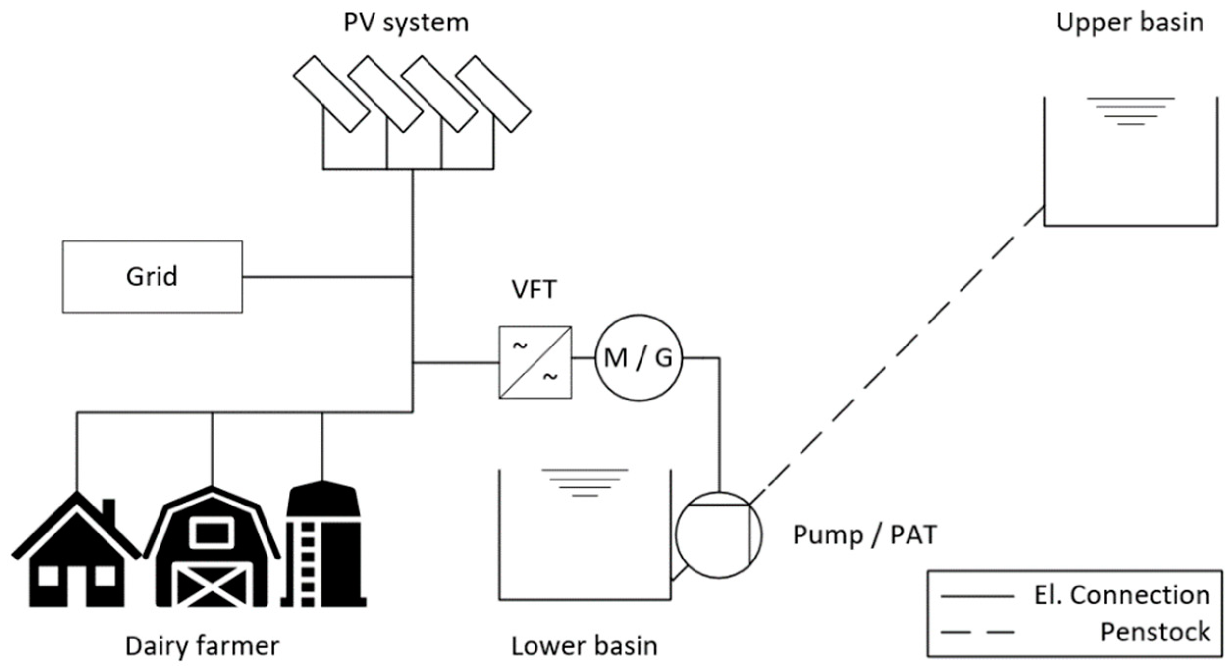
2. Micro-Hydro Storage System and Operating Strategies

Figure 1 presents a diagram of a speed-controlled micro pump storage plant that might be used by a small company (e.g., a dairy farmer). A centrifugal pump, which operates both as a pump and a turbine is located between the lower and the upper basins. The plant is connected to the grid, a PV system (specific yield = $1.15\frac{\mathrm{kWh}}{\mathrm{kWp}}$), and the consumer via an electric motor or generator (M/G) and a frequency converter. In contrast to pump maps, turbine maps are rarely provided by manufacturers. Therefore, as a first scenario, we aimed to find the best possible location for a given pump (where turbine maps are available) under certain framework conditions. The component selected was a KSB50160 centrifugal pump (made by KSB AG (Frankenthal, Germany)). Furthermore, the penstock was assumed to have a nominal diameter of DN150 and a slope of 15%. The summed value of the pressure loss coefficients ${\zeta }_{fit}$ of all the fittings is ${\zeta }_{tot}=0.50$ whereby the individual loss coefficients ${\zeta }_{fit}$ are defined by [35] as

$${\zeta }_{fit}=\frac{\Delta p}{\frac{\rho }{2}\cdot v^2},$$

(1)

where $\Delta p$ is the pressure loss in the fitting and $v$ the water velocity.

A snow-making style of water reservoir design was assumed, similar to the water storage facility that was recently built in the Unterstmatt ski resort [36,37]. There, the installation effort on site was minimized by using prefabricated geomembranes to realize a cost-effective in-ground basin.

To familiarize the reader with the functionality of the system, Figure 2 presents the simulated power balance of a day in February 2014. It shows the operating mode of a speed-controlled micro pump storage plant with the measured load profile of a dairy farmer. In pump operation ($P_{Pump}>0$), at low energy consumption ($P_{L1}$) and high solar energy production ($P_{PV}$), water is pumped into an upper reservoir, with the current water volume ($V$) in the upper basin corresponding to energy stored for later use. During times of high-power consumption and low PV output, the turbine operation ($P_{Turb}>0$) mode is active, and is characterized by water flowing back to the lower basin and driving the centrifugal pump, which now acts as a turbine.

2.1. Operating Strategies

There are various operating modes (OP mode) available for a pumped-storage power plant. This paper briefly presents and evaluates three of them, focusing on the technical and economic aspects. The operating strategies include the fixed operating point, speed control, and throttle control.

2.1.1. Fixed Operating Point

The first option is to run the centrifugal pump at a fixed operating point, as defined by the fixed flow rate and rotational speed, with the latter being given by the grid frequency and the number of pole pairs in the electric motor. For example, to operate the generator at 50 Hz grid frequency, it is necessary to run the centrifugal pump at a given speed of, for instance, 1500 rpm (with two-pole pairs) [38]. For this purpose, an asynchronous motor is used to connect the system directly to the power grid. This is less expensive than a synchronous motor but has the disadvantage of having lower efficiency, especially with partial load. As the pump and turbine maps differ, a compromise in the selection of components must be found that enables a good combination of the individual efficiencies of the pump and the turbine modes and results in the best possible combined efficiency.

2.1.2. Throttle Control

Another frequently used option is throttle control. Figure 3 shows a turbine map including the speed curves ($n$ = 1400–3900 rpm) and the concept of throttle control, based on the example of a PAT in turbine operation. By adjusting a valve in the pressure line, the system’s characteristic curve (red) can be changed from AP1 to AP2 to achieve the required flow rate and pressure head. Due to its low investment costs, this method is favored for small to medium-sized machines. Turbine power loss ($P_v$) caused by the throttle as a loss of head ($\Delta H_{DRV}$) is defined by:

$$P_v=\rho gQ\Delta H_{Loss}\cdot \eta$$

(2)

A major disadvantage of throttle control is that pumps may operate well below their ultimate efficiency point, which increases the risk of excess wear, cavitation damage, noise, and vibration [39].

2.1.3. Speed Control with a Frequency Converter

The disadvantages of throttle control, particularly the significant throttling losses involved, can be overcome by using speed control (Figure 4). By controlling the speed with a frequency converter, the working point can be moved anywhere along the system’s characteristic curve (e.g., from AP1 to AP2 and vice versa). A significant improvement in efficiency can be achieved, particularly in the case of a steep system’s characteristic curves. Vibration-inducing forces and the risk of cavitation are reduced by running speed-controlled pumps at reduced speed and partial load. Speed control, therefore, protects the pump and any valves and tends to be more economical than throttle control in terms of maintenance costs. However, it should be noted that investment and frequency converter maintenance costs also need to be taken into account. Therefore, only the additional investment and maintenance costs of the frequency transformer stand in the way of the broad application of speed control.

2.2. The Simulation Model

To investigate and compare the technical and economic properties of the different pump and turbine control regimes, a detailed simulation model for the whole system was drawn up. This subsection presents the structure and functionality of the model.

2.2.1. Inputs and Basic Data

Figure 5 shows the inputs and outputs for the simulation model. An additional continuously variable motor is provided on the control valve for throttle control. Due to its high efficiency in the partial load range, we assumed that a synchronous motor would be used for speed control. An asynchronous motor was chosen for throttle control and the fixed operating point mode. Measured performance data from a PV system in southern Germany were used for modeling the PV power output [40]. A dairy farm was chosen as an exemplary test case, whose electrical load requirement was represented by a measured load profile provided by the Bavarian State Institute for Agriculture [41]. The pump and turbine maps, including the performance data required for the simulation, were delivered in graphic form by KSB Aktiengesellschaft [42] and were subsequently digitized. Similarly, the efficiency maps of the synchronous [43] and asynchronous motor [44] were also converted.

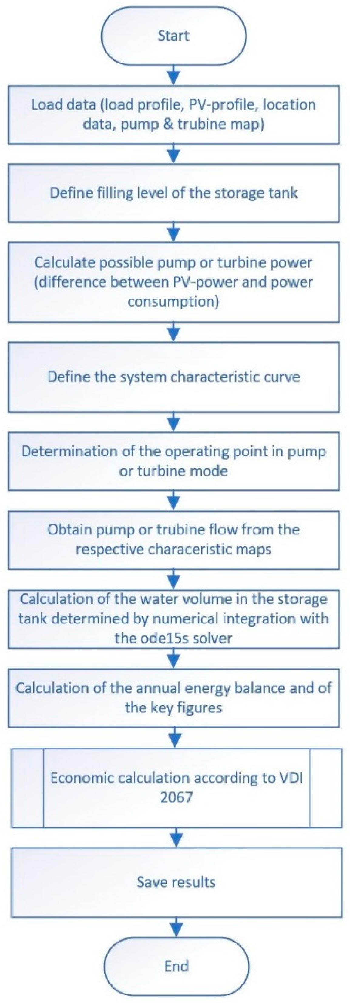
2.2.2. Program Sequence

A detailed description of the program sequence (Figure 6) is provided as follows. After initiating the simulation, all the required data, as shown on the left side of Figure 5, are gathered by the program. The relationship between the water volume $V$ in the storage reservoir to the pump and the turbine flow through the PAT ($Q_{pump}$ and $Q_{turb}$, respectively) is given by the following ordinary differential equation:

$$\dot{V}= Q_{pump}-Q_{turb}$$

(3)

It should be noted that no external water inflow or evaporation is considered. To solve this numerically, $Q_{pump}$ and $Q_{turb}$ have to be obtained from characteristic maps. There is a set of two maps each for the turbine and pump operation, respectively. The map $H_{turb}(Q_{turb},n)$ represents the dependency of head $H_{turb}$ on flow and speed, while the second map $P_{turb}$ ($Q_{turb},n$) shows the power (from which the efficiency can also be obtained). Accordingly, pump operation is described by $H_{pump}$($Q_{pump},n$) and $P_{pump}$($Q_{pump},n$).

The difference between PV power and power from the load profile $P_{Pv/L1}= P_{Pv}- P_{L1}$ results in the possible pump $P_{pump}(Q_{pump},n)$ or turbine $P_{turb}(Q_{turb},n)$ power depending on the flow and speed and taking into account the efficiency of the electrical components in the drive unit ${\eta }_{el}$:

$$P_{pump}^{mech }=P_{Pv/L1}\cdot {\eta }_{el}$$

(4)

$$P_{turb}^{mech}=\frac{-P_{Pv/L1}}{{\eta }_{el}}$$

(5)

To determine the resulting head, taking pipe losses $h_f$ into account, the system’s characteristic curves $H{(\dot{V})}_{pump} \mathrm{and} H{(\dot{V})}_{turb}$ have to be defined. The curves depend on the flow $\dot{V}$, the Darcy friction factor $f_D$, the dynamic loss coefficient ${\zeta }_{tot},$ gravitational acceleration $g,$ pipe length $L_{pipe}$ and diameter $d_N$ [44,45]:

$$H_{pump}(\dot{V})=H_{geo}+\left[f_D(\dot{V})\cdot \frac{L_{pipe}}{d_N}+{\zeta }_{tot}\right]\frac{{(\frac{4\cdot \dot{V}}{3600s/h\cdot \pi \cdot d_{N^2}})}^2}{2\cdot g}$$

(6)

$$H_{turb}(\dot{V})=H_{geo}-\left[f_D(\dot{V})\cdot \frac{L_{pipe}}{d_N}+{\zeta }_{tot}\right]\frac{{(\frac{4\cdot \dot{V}}{3600s/h\cdot \pi \cdot d_{N^2}})}^2}{2\cdot g}$$

(7)

The operating point ($Q_i$,n) is now determined by numerically solving the following equations:

$$P_i(Q_i,n)=P_i^{mech}$$

(8)

$$H_i(Q_i,n)=H_i(\dot{V})$$

(9)

where $i=turb$ for turbine mode and $i=pump$ for pump mode, respectively.

Graphically, this corresponds to the intersection of the system’s characteristic curve $H_i(Q_i)$ (see for example, the red line in Figure 4) with the turbine or pump power isoline (violet lines) corresponding to the power $P_i^{mech}$. The flow rate and speed at the intersection point can then be read directly from the characteristic maps.

The limit values of pump or turbine operation are the lines for maximum $n_{max}$ and minimum speed $n_{min}$, as well as the line for minimum $Q_{\min }$ and maximum flow $Q_{\max }$ (Figure 4). It is also important to provide hysteresis to prevent the turbine from shutting down immediately after starting due to a small drop in load request.

In total, the water volume of the storage tank is determined by numerical integration, and the states “storage tank full” and “empty” are defined. The simulation model provides results for every point in the time of year for all system variables, such as storage level, turbine and pump flow, power, and so on. The annual electricity balance can then be obtained from these results and a profitability calculation can be performed.

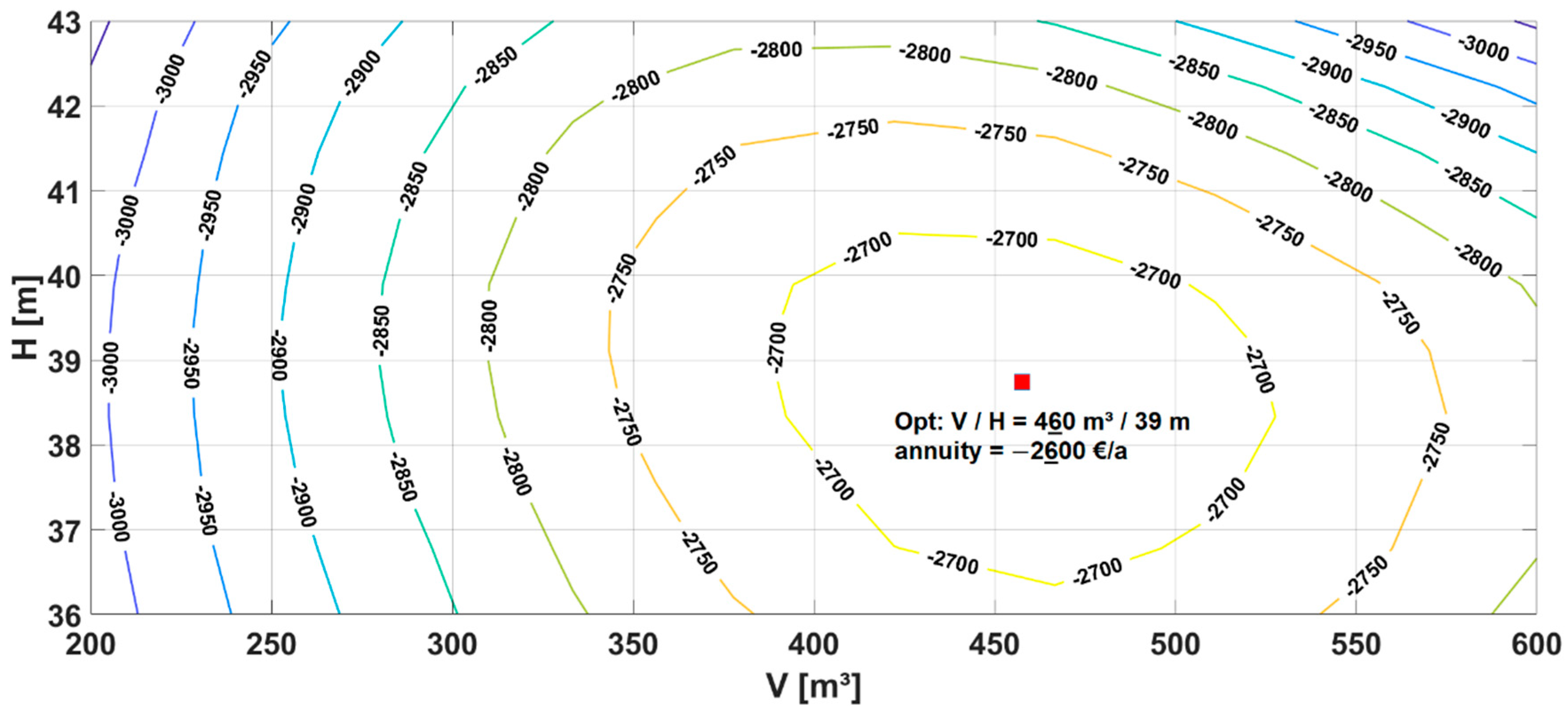
2.2.3. Finding the Optimal Site

The simulation model was employed to determine an optimal site (as defined by the available head $H$ and storage tank volume $V$) for a given PAT. By using the integrated MATLAB 2019a simulated annealing algorithm [46,47], the economical outcome represented by the annuity (see Section 3) can be maximized by varying $H_{geo}$ and $V$. This optimization can take more than two days, depending on the computational power of the PC (e.g., 6 h with an Intel i7-8700K using a single core). The results for the optimal site ($H_{opt}, V_{opt}$) are obviously specific to the PAT type chosen for the simulation model (here 50160D174) and are shown in

Table 1. Technical results for pump storage, including optimized storage volume ($V_{opt}$), optimized head ($H_{opt}$), total efficiency (${\eta }_{tot}$), average pump efficiency (${\eta }_{p\_m}$), average turbine efficiency (${\eta }_{t\_m}$), number of pump activations ($Pum{p}_{on}$), number of turbine activations ($Tur{b}_{on}$), maximum power in pump mode ($P_{max}$), storage capacity, and degree of self-sufficiency.

OP Mode	${\mathit{V}}_{\mathit{o}\mathit{p}\mathit{t}}$	${\mathit{H}}_{\mathit{o}\mathit{p}\mathit{t}}$	${\mathit{\eta }}_{\mathit{t}\mathit{o}\mathit{t}}$	${\mathit{\eta }}_{\mathit{p}\_\mathit{m}}$	${\mathit{\eta }}_{\mathit{t}\_\mathit{m}}$	$\mathit{P}\mathit{u}\mathit{m}{\mathit{p}}_{\mathit{o}\mathit{n}}$	$\mathit{T}\mathit{u}\mathit{r}{\mathit{b}}_{\mathit{o}\mathit{n}}$	${\mathit{P}}_{\mathit{m}\mathit{a}\mathit{x}}$	Storage Capacity	Degree of Self-Sufficiency
Speed control	460 m3	39 m	42%	68%	62%	860	1000	13 kW	48 kWh	50%
Throttle control	280 m3	42 m	30%	63%	47%	850	990	12 kW	32 kWh	43%
Fixed OP	300 m3	44 m	35%	62%	57%	920	760	10 kW	36 kWh	44%

.

3. Results and Discussion

This section presents and discusses the technical and economic results of the simulation. The aim of the optimization was to maximize the economic efficiency for each of the three control strategies and compare the results.

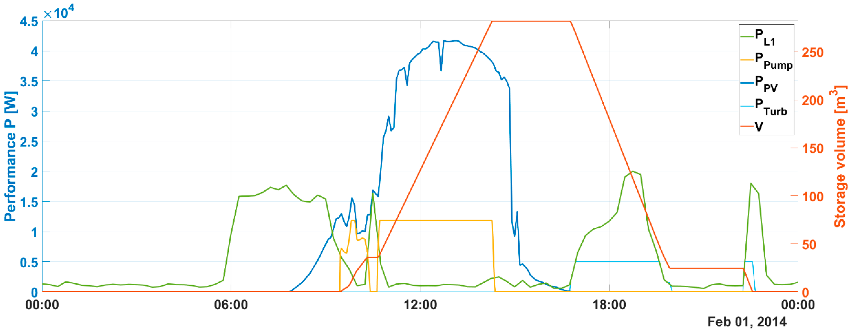
3.1. Technical Results and Discussion

Table 1 shows the technical results for the pump storage. Many of these results were not unexpected.

For speed control, an ideal site would have an optimal head $H_{opt}$ of 39 m and an optimal storage volume $V_{opt}$ of 460 m³. Speed control obtains both the highest efficiency and the best degree of self-sufficiency, which is defined based on the energy obtained from the grid $W_{grid}$ and the total energy requirement $W_{Load}$:

$$\mathrm{degree}\mathrm{of}\text{ self-sufficiency }=1-\frac{W_{grid}}{W_{load}}\cdot 100\%$$

(10)

On average, speed control also has the best pump and turbine efficiency. The throttle control strategy shows the lowest total efficiency ${\eta }_{tot}$, which is defined as the quotient of the total electrical energy output $W_{out}$ and the total electrical energy input $W_{in}$ [48]:

$${\eta }_{tot}=\frac{W_{out}}{W_{in}}\cdot 100\%$$

(11)

Throttle control displays a similar degree of self-sufficiency to that of the fixed OP. The increased number of activations (Table 1) of the turbine $Tur{b}_{on}$ reveals that this operating mode has higher flexibility compared to fixed OP. Throttle control achieves its optimum at a storage volume $V_{opt}$ of 280 m³ and a head $H_{opt}$ of 42 m. The third operating mode, fixed OP, has a combined efficiency of the pump and turbine mode ${\eta }_{tot}$ of 35%, placing it between the other two alternatives. In this mode, it is essential to select a centrifugal pump that achieves the best possible combination of pump and turbine efficiencies at the given motor speed. The resulting self-sufficiency is the lowest value of all the alternatives considered. Compared to a self-sufficiency of 34% for the PV-system alone, the application of the micro pump storage results in an increase of 10 to 16 percentage points, depending on the chosen operating mode.

3.2. Economic Results and Discussion

The annuity method according to VDI 2067 [49] was employed to assess economic efficiency. It is one of several widely used procedures for assessing the performance of investments. It allows the annuity of a one-time investment to be determined at the beginning of a project, as well as the ongoing costs during the evaluation period. Data for lifetimes and maintenance were taken from VDI 2067 (except for the maintenance and support costs of the frequency inverter over its service life). Our analysis was based on a period of 30 years, and reinvestment and residual value were also taken into account over this time according to the formulae given in Appendix A.

Since the present analysis focuses on the continued use of an existing PV system after the expiry of EEG remuneration, the investment in the PV system itself is not relevant and therefore it was set as a baseline. Furthermore, it was assumed that out of the two required reservoirs, one already exists and the other needs to be built at a specific cost of 40 €/m³. The annual discount rate and price increase were set to 2.0% each.

Table 2. Investment costs per unit for storage ($I_{0\_stor}$), penstock ($I_{0\_pen}$), pump ($I_{0\_pump}$), drive unit ($I_{0\_el}$), control valve ($I_{0\_thrott}$), other costs ($I_{0\_oth}$) and total investment for the system ($I_{0\_tot}$).

OP Mode	${\mathit{I}}_{0\_\mathit{s}\mathit{t}\mathit{o}\mathit{r}}$	${\mathit{I}}_{0\_\mathit{p}\mathit{e}\mathit{n}}$	${\mathit{I}}_{0\_\mathit{e}\mathit{l}}$	${\mathit{I}}_{0\_\mathit{P}\mathit{u}\mathit{m}\mathit{p}}$	${\mathit{I}}_{0\_\mathit{t}\mathit{h}\mathit{r}\mathit{o}\mathit{t}\mathit{t}}$	${\mathit{I}}_{0\_\mathit{o}\mathit{t}\mathit{h}}$	${\mathit{I}}_{0\_\mathit{t}\mathit{o}\mathit{t}}$
Speed control	40 €/m3	50 €/m	16,000 €	3800 €	1000 €	5000 €	56,000 €
Throttle control	40 €/m3	50 €/m	7200 €	3800 €	2500 €	5000 €	44,000 €
Fixed OP	40 €/m3	50 €/m	7200 €	3800 €	1000 €	5000 €	44,000 €

shows the investment costs $I_0$ for the individual components of the pumped-storage power plant, including the German value-added tax (VAT) rate of 19%. List prices of various manufacturers were used to determine the investment. Total investment costs $I_{0\_tot}$ are the sum of the individual investment costs. As can be seen, fixed OP and throttle control incur lower investment costs then speed control. The additional charges incurred with speed control are due to the frequency converter and synchronous motor. The cost of a frequency converter is normally in the same range as the cost of the generator. For throttle control, an additional continuously variable motor is provided on the control valve.

3.2.1. Annuity Calculation Results for Speed Control

Figure 7 shows the dependency of annuity on the variable parameters of head $H$ and reservoir volume $V$ for an electricity purchase price of 31.9 cents. Annual annuity reaches its maximum value of −2600 € at a head of about 39 m and a reservoir volume of about 460 m³. It is interesting to note that a slight change in the head of around 37–40 m only has a small impact (<100 €) on the annual annuity. Similarly, a change in the size of the storage volume in the range of around 400 to 500 m³ has the same small effect on the annuity.

3.2.2. Annuity Calculation Results for the Fixed OP

In the corresponding plot for fixed OP (Figure 8), changes in the amount of H- and V-variation only have a slight impact on the annual annuity, which is similar to the results for speed control. The optimum storage tank size for the fixed OP is 300 m³, which is considerably smaller than for speed control, while the optimum head increases to approximately 44 m with an annual annuity of −2200 €.

3.2.3. Annuity Calculation Results for Throttle Control

Throttle control (Figure 9), which displayed the poorest technical results, actually outperforms speed control when it comes to economic considerations. The additional investment costs (mainly for the frequency transformer) do not pay off at the current electricity price. Again, annuity changes only slightly when the head is varied. The optimum level is reached for a head of around 42 m and a storage volume of about 280 m³, resulting in an annual annuity of −2500 €/kWh. The optimization results for an electricity price of 31.9 cents /kWh show that pumped storage as presented is not profitable for any operation mode at that price. Particularly for speed control, the additional investment costs are currently not cost-effective, but this would change with increasing energy procurement costs, as will now be shown.

3.2.4. Sensitivity Analysis and Comparison of the Different Operating Modes with Increasing Energy Procurement Costs

Figure 10 shows annual annuity as a function of electricity price, with H and V set to their respective optimized values, as given in Table 1. Unsurprisingly, the economic situation changes significantly with increasing electricity prices. It is interesting to note that throttle control is never the preferred solution while using the fixed OP strategy is the best option when the electricity price is low, under these circumstances, it basically only serves to limit financial loss. For higher prices (starting from about 0.45 €/kWh), speed control becomes the best operating mode and is the first to reach a profitability threshold at 0.59 €/kWh.

To assess the impact of various parameters on the outcome of our analysis, we performed a sensitivity analysis, in which variations in the cost of storage, PAT, pipeline and drive unit were investigated. The results are presented in Figure 11 and show that the drive unit (i.e., the motor/generator together with the VFT and feed-in unit) has the greatest impact on the annual annuity. Changing reservoir and piping prices has a similar but smaller impact, while the cost of the PAT has the smallest effect on the annual annuity.

3.2.5. LCOE Calculation and Comparison with Other Scientific Research Findings

The storage in Froyennes has an LCOE around 1.06 €/kWh [23] and the result for storage tanks in buildings was 1.66 €/kWh [24]. To enable comparison with these findings, the LCOE for the micro-pump storage under consideration here was calculated using the following formula [50]:

$$LCOE=\frac{I_0 + {{\displaystyle \sum }}_{t=1}^n\frac{A_t}{{(1+i)}^t}}{{{\displaystyle \sum }}_{t=1}^n\frac{W_{t, el}}{{(1+i)}^t}}$$

(12)

In year zero $t$, in which the plant is established, all investment costs are considered as $I_0$, and no energy $W_{t, el}$ is drawn from the pumped storage. For any given year t between one and the final year, the sum of costs $A_t$ consists of the operating and maintenance costs $O\&M_t$, the possible sale of electricity on the electricity exchange $E{S}_t$, and reinvestment for replacement purchases $R{I}_t$. In the final year, the residual values of the components $R{W}_t$ are also taken into account and deducted from the costs:

$$A_t=O\&M_t+E{S}_t+R{I}_t-R{W}_t$$

(13)

As with the annuity method, the discount rate i is set to 2 %. This results in an LCOE of around 0.63 €/kWh for speed control, 0.74 €/kWh for the fixed OP, and 0.85 €/kWh for throttle control. This confirms the results in Figure 10, and shows that speed control is the best choice for ensuring economical operation. Since the choice of the interest factor is usually based on the user’s expectations, the results of the LCOE calculation for different interest factors are shown in

Table 3. The levelized cost of energy (LCOE) for different interest rates.

Interest Rate	$2\mathit{\%}$	$4\mathit{\%}$	$6\mathit{\%}$	$8\mathit{\%}$
Speed control	0.63 €/kWh	0.74 €/kWh	0.86 €/kWh	0.98 €/kWh
Throttle control	0.85 €/kWh	0.99 €/kWh	1.16 €/kWh	1.33 €/kWh
Fixed OP	0.74 €/kWh	0.87 €/kWh	1.01 €/kWh	1.17 €/kWh

.

4. Conclusions and Outlook

This paper employed a detailed techno-economic simulation model of a micro-hydro storage, and demonstrated that good economic results can be achieved with sufficient head and a short distance between the reservoirs. Compared to the LCOE for the storage in Froyennes, which was around 1.06 €/kWh (see Section 1) and a storage tank in buildings with an LCOE of 1.66 €/kWh (see Section 1), the results obtained here, e.g., 0.63 €/kWh obtained for speed control, are very promising. Considering the technical results, it is clear that speed control with a frequency transformer is the best operating mode. However, once the economic results are also taken into account, it is no longer that simple. Even if speed control with an LCOE of 0.63 €/kWh seems to be the most economically efficient operating mode, taking the electricity purchase costs in the annuity analysis into consideration, it is clear that this is not the case at the current energy prices. However, if energy prices increase, speed control quickly becomes the most economical operating mode. The additional investment cost payoff and speed control outperforms throttle control at an electrical power purchase price of around 0.35 €/kWh; for the fixed OP, this happens around 0.45 €/kWh (Figure 10).

This paper identified the optimal location for a specific centrifugal pump. In reality, the aim is usually to identify the best possible centrifugal pump for a particular location. For this reason, a test bench for measuring turbine characteristic maps of various centrifugal pumps is currently being set up in cooperation with Herborner Pumpen GmbH (Herborn, Germany) and the engineering company, Pfeffer (Regen, Germany). This test bench will enable the creation of a database for pump and turbine characteristics. Furthermore, the simulation model will be modified to determine the most suitable pump for enabling economical operation at a certain location. Moreover, other pump turbines, such as the promising Deriaz-PAT [51] could be included in the database.

References

1. Photovoltaics Report. Available online: https://www.ise.fraunhofer.de/content/dam/ise/de/documents/publications/studies/Photovoltaics-Report.pdf (accessed on 1 June 2020).
2. Photovoltaik-Anlagen Dürfen Nach Ende der EEG-Förderung Nicht Einfach Wild Einspeisen. Available online: https://www.pv-magazine.de/2019/08/01/pv-anlagen-duerfen-nach-ende-der-eeg-foerderung-nicht-einfach-wild-einspeisen/ (accessed on 1 June 2020).
3. Stock Market Electricity Price at EPEX-Spot Market for Germany/Austria and Germany/Luxemburg. Available online: https://de.statista.com/statistik/daten/studie/289437/umfrage/strompreis-am-epex-spotmarkt/ (accessed on 1 June 2020).
4. Bundesnetzsagentur; Bundeskartellamt. Bundesnetzagentur—Monitoringbericht 2019. 2020, p. 298. Available online: https://bundesnetzagentur.de/SharedDocs/Mediathek/Berichte/2019/Monitoringbericht_Energie2019.pdf (accessed on 1 June 2020).
5. Strompreise* für Haushalte in den Ländern der EU-28 im Jahr 2018. Available online: https://de.statista.com/statistik/daten/studie/197196/umfrage/elektrizitaetspreise-ausgewaehlter-europaeischer-laender/ (accessed on 1 June 2020).
6. Ramos, M.H.; Dadfar, A.; Basharat, M.; Adeyeye, K. Inline pumped storage hydropower towards smart and flexible energy recovery in water networks. Water 2020, 12, 2224. [Google Scholar] [CrossRef]
7. De Marchis, M.; Fontanazza, C.M.; Freni, G.; Messineo, A.; Milici, B.; Napoli, E.; Notaro, V.; Puleo, V.; Scopa, A. Energy recovery in water distribution networks. Implementation of pumps as turbine in a dynamic numerical model. Procedia Eng. 2014, 70, 439–448. [Google Scholar] [CrossRef] [Green Version]
8. Carravetta, A.; Del Giudice, G.; Fecarotta, O.; Ramos, M.H. Pump as Turbine (PAT) design in water distribution network by system effectiveness. Water 2013, 5, 1211–1225. [Google Scholar] [CrossRef] [Green Version]
9. Fecarotta, O.; Ramos, H.; Derakhshan, S.; Del Giudice, G.; Carravetta, A. Fine tuning a PAT hydropower plant in a water supply network to improve system effectiveness. J. Water Resour. Plan. Manag. 2018, 144, 04018038. [Google Scholar] [CrossRef]
10. Ramos, H.; McNabola, A.; Lopez-Jimenez, P.A.; Perez-Sanchez, M. Smart water management towards future water sustainable networks. Water 2020, 12, 58. [Google Scholar] [CrossRef] [Green Version]
11. Carravetta, A.; Del Giudice, G.; Fecarotta, O.; Ramos, H. Energy production in water distribution networks: A PAT design strategy. Energies 2013, 6, 411–424. [Google Scholar] [CrossRef] [Green Version]
12. Madeira, C.F.; Fernandes, F.P.J.; Perez-Sanchez, M.; Lopez-Jimenez, P.A.; Ramos, M.H.; Branco, P.J.C. Electro-hydraulic transient regimes in isolated pumps working as turbines with self-excited induction generators. Energies 2020, 13, 4521. [Google Scholar] [CrossRef]
13. Stepanoff, A.J. Centrifugal and Axial Flow Pumps, Design and Applications, 2nd ed.; John Wiley and Sons, Inc.: Hoboken, NJ, USA, 1957; Available online: https://wrap.warwick.ac.uk/36099/ (accessed on 1 June 2020).
14. Gülich, J.F. Turbinenbetrieb. Allgemeines kennfeld. In Kreiselpumpen; Springer: Berlin/Heidelberg, Germany, 2013; Volume 4, pp. 847–870. [Google Scholar]
15. Alatorre-Frenk, C. Cost Minimization in Microhydro Systems Using Pumps-as-Turbines. Ph.D. Thesis, University of Warwick, Coventry, UK, 1994; pp. 55–113. [Google Scholar]
16. Derakhshan, S.; Nourbakhsh, A. Experimental study of characteristic curves of centrifugal pumps working as turbine in different specific speeds. Exp. Therm. Fluid Sci. 2008, 32, 800–807. [Google Scholar] [CrossRef]
17. Yang, S.; Derakhshan, S.; Kong, F. Theoretical, numerical and experimental prediction of pump as turbine performance. Renew. Energy 2012, 48, 507–513. [Google Scholar] [CrossRef]
18. Pugliese, F.; De Paola, F.; Fontana, N.; Giugni, M.; Marini, G. Experimental characterization of two Pumps as Turbines. Renew. Energy 2016, 99, 180–187. [Google Scholar] [CrossRef]
19. Stefanizzi, M.; Torresi, M.; Fortunato, B.; Camporeale, S.M. Experimental investigation and performance prediction modeling of a single stage centrifugal pump operation as turbine. Energy Procedia 2017, 126, 589–596. [Google Scholar] [CrossRef]
20. Barbarelli, S.; Amelio, M.; Florio, G. Experimental activity at test rig validation correlations to select pumps running as turbines in micro hydro plants. Energy Convers. Manag. 2017, 149, 781–797. [Google Scholar] [CrossRef]
21. Anilkumar, T.T.; Simon, S.P.; Padhy, N.P. Residential electricity cost minimization model through open well-pico turbine pumped storage system. Appl. Energy 2017, 195, 23–35. [Google Scholar] [CrossRef]
22. Morabito, A.; Steimes, J.; Bontems, O.; Al Zohbi, G.; Hendrick, P. Set-up of a pump as turbine use in micro-pumped hydro energy storage: A case study in Froyennes Belgium. J. Phys. Conf. Ser. 2017, 813, 012033. [Google Scholar] [CrossRef]
23. Morabito, A.; Hendrick, P. Pump as turbine applied to micro energy storage and smart water grids: A case study. Appl. Energy 2019, 241, 567–579. [Google Scholar] [CrossRef]
24. de Oliveira e Silva, G.; Hendrick, P. Pumped hydro energy storage in buildings. Appl. Energy 2016, 179, 1242–1250. [Google Scholar] [CrossRef]
25. Borkowski, D. Analytical model of small hydropower plant working at variable speed. IEEE Trans. Energy Convers. 2018, 33, 1886–1894. [Google Scholar] [CrossRef]
26. Barbarelli, S.; Amelio, M.; Florio, G. Predictive model estimating the performances of centrifugal pumps used as turbines. Energy 2016, 107, 103–121. [Google Scholar] [CrossRef]
27. Vasudevan, K.R.; Ramachandaramurthy, V.K.; Gomathi, V.; Ekanayake, J.B.; Tiong, S.K. Modelling and simulation of variable speed pico hydel energy storage system for microgrid applications. J. Energy Storage 2019, 24, 100808. [Google Scholar]
28. Mohanpurkar, M.; Ouroua, A.; Hovsepian, R.; Luo, Y.; Singh, M.; Muljadi, E.; Gevorgian, V.; Donalek, P. Real-time co-simulation of adjustable-speed pumped storage hydro for transient stability analysis. Electr. Power Syst. Res. 2018, 154, 276–286. [Google Scholar] [CrossRef]
29. Schmidt, J.; Kemmetmüller, W.; Kugi, A. Modeling and static optimization of a variable speed pumped storage power plant. Renew. Energy 2017, 111, 38–51. [Google Scholar] [CrossRef]
30. Stoppato, A.; Benato, A.; Destro, N.; Mirandola, A. A model for the optimal design and management of a cogenartion system with energy storage. Energy Build. 2016, 124, 241–247. [Google Scholar] [CrossRef]
31. Ma, T.; Yang, H.; Lu, L.; Peng, J. Pumped storage-based standalone photovoltaic power generation system: Modeling and techno economic optimization. Appl. Energy 2015, 137, 649–659. [Google Scholar] [CrossRef]
32. Yang, W.; Yang, J. Advantage of variable-speed pumped storage plants for mitigating wind power variations: Integrated modelling and performance assessment. Appl. Energy 2019, 237, 720–732. [Google Scholar] [CrossRef]
33. Simao, M.; Ramos, H. Hybrid pumped hydro storage energy solutions towards wind and PV integration: Improvement on flexibility, reliability and energy costs. Water 2020, 12, 2457. [Google Scholar] [CrossRef]
34. Morabito, A.; Furtado, A.; Gilton, C.; Hendrick, P. Variable speed regulation for pump as turbine in micro pumped hydro energy storage. In Proceedings of the 38th IAHR World Congress, Panama City, Panama, 1–6 September 2019. [Google Scholar]
35. Recknagel, H.; Sprenger, E.; Schramek, E.-R. Taschenbuch für Heizung + Klimatechnik; Oldenbourg Industrieverlag: München, Germany, 2008. [Google Scholar]
36. Beschneiungsanlage Erhält Wasserspeicher. Available online: https://bnn.de/lokales/abb/beschneiungsanlage-erhaelt-waserspeicher (accessed on 30 April 2020).
37. Fahrner, H.; (Nationalpark-Hotel Schliffkopf, Schliffkopf, Germany); Lugauer, F.J.; (TUM Campus Straubing for Biotechnology and Sustanability, Weihenstephan-Triesdorf University of Applied Science, Straubing, Germany). Personal communication, 2020.
38. Carravetta, A.; Houreh, D.S.; Ramos, H. Rotational speed selection. In Pumps as Turbine; Springer Nature: Cham, Switzerland, 2018; p. 87. [Google Scholar]
39. Gülich, J.F. Verhalten der Kreiselpumpen in Anlagen. In Kreiselpumpen; Springer: Berlin/Heidelberg, Germany, 2013; Volume 4, pp. 809–814. [Google Scholar]
40. Kainz, J.; (TUM Campus Straubing for Biotechnology and Sustanability, Weihenstephan-Triesdorf University of Applied Science, Straubing, Germany); Lugauer, F.J.; (TUM Campus Straubing for Biotechnology and Sustanability, Weihenstephan-Triesdorf University of Applied Science, Straubing, Germany). Personal communication, 2018.
41. Neser, S. Energiebedarf und Einsparmöglichkeiten in der Rinderhaltung; Bayerische Landesanstalt für Landwirtschaft (LfL): Freising, Germany, 2014; Volume 1, pp. 7–22. [Google Scholar]
42. Vorpahl, L.; (KSB SE & Co. KGaA, Frankenthal, Germany); Huber, B.; (TUM Campus Straubing for Biotechnology and Sustanability, Straubing, Germany). Personal communication, 2017.
43. MAX LAMB GMBH & CO. KG, KAT-ABSRIE-0415. Available online: https://www.lamb.de/fileadmin/KAT-ABSRIE-0415.pdf (accessed on 28 January 2020).
44. KSB Aktiengesellscahft. Selecting Centrifugal Pumps; KSB Aktiengesellschaft: Frankenthal, Germany, 2005; Volume 4, pp. 19–31. [Google Scholar]
45. Menny, K. Strömungsmaschinen; Teubner: Wiesbaden, Germany, 1985; ISBN 978-3-519-06317-9. [Google Scholar]
46. Kirkpatrick, S.; Gelatt, C.D., Jr.; Vecchi, M.P. Optimization by simulated annealing. Science 1983, 220, 671–680. [Google Scholar] [CrossRef]
47. Mathworks. Global Optimization Toolbox: Simulated Annealing (r2019a). Available online: https://de.mathworks.com/help/gads/simulannealbnd.html (accessed on 28 January 2020).
48. Quaschning, V. Wasserkraft. Regenerative Energiesysteme; Carl Hanser Verlag: Munich, Germany, 2015; Volume 9, pp. 327–346. [Google Scholar]
49. Association of German Engineers. Economic Efficiency of Building Installations—Fundamentals and Economic Calculation; Verein Deutscher Ingenieure e.V.: Düsseldrof, Germany, 2012; pp. 29–36. [Google Scholar]
50. Branker, K.; Pathak, M.J.M.; Pearce, J.M. A review of solar photovoltaic levelized cost of electricity. Renew. Sustain. Energy Rev. 2011, 15, 4470–4482. [Google Scholar] [CrossRef] [Green Version]
51. Morabito, A.; de Olivia e Silvia, G.; Hendrick, P. Deriaz-pump-turbine for pumped hydro energy storage and micro applications. J. Energy Storage 2019, 24, 100788. [Google Scholar] [CrossRef]
Figure 1. Concept of a micro-pump storage power plant using the example of a dairy farmer.
Energies 14 00425 g001
Figure 2. Exemplary simulated power balance of the speed controlled micro pump storage plant including load profile ( P L 1 ), pump power ( P P u m p ), PV power ( P P V ), turbine power ( P T u r b ) and the storage volume ( V ).
Energies 14 00425 g002
Figure 3. Throttle control with the example of a KSB50160 centrifugal pump in turbine operation.
Energies 14 00425 g003
Figure 4. Speed control based on the example of turbine operation with a KSB50160 pump.
Energies 14 00425 g004
Figure 5. Inputs (left) and outputs (right) of the simulation model.
Energies 14 00425 g005
Figure 6. Flow chart of simulation model.
Energies 14 00425 g006
Figure 7. Dependency of annuity with speed control.
Energies 14 00425 g007
Figure 8. Dependency of annuity with a fixed operating point (OP).
Energies 14 00425 g008
Figure 9. Dependency of annuity with throttle control.
Energies 14 00425 g009
Figure 10. Comparison of annual annuity with rising electricity procurement costs.
Energies 14 00425 g010
Figure 11. Sensitivity analysis for storage, the pump-as-turbine (PAT), drive unit and pipeline costs.
Energies 14 00425 g011