Optimal Voltage Control in MV Network with Distributed Generation

Abstract

The article presents the concept of voltage control in a medium-voltage network, using the classical control of a HV/MV (High Voltage/Medium Voltage) transformer and active participation of distributed generation sources. The proposed solution is based on the results of the optimization process. The objective function is considered as a single-criterion—the voltage quality indicator or value of power losses in the network, and optionally as two-criteria (voltage quality and losses combined, with appropriately selected weight factors). The analysis carried out for random selection of independent variables, using the original heuristic algorithm, indicated a very high efficiency of the proposed control process, compared to the traditional approach. A significant improvement in the voltage quality index and reduction of losses was found, which justifies the advisability of looking for new solutions in the field of voltage control in MV networks, taking into account active participation of distributed generation.

1. Introduction

Power networks are becoming increasingly saturated with distributed sources. Most often, they are wind and photovoltaic farms; in addition, the number of biogas plants is increasing. A significant number of these sources, especially in medium- and low-voltage networks, contribute to voltage problems. Grids, which until now, have worked as receiving networks, periodically become supply networks. Their basic supply from HV/MV transformers becomes supported by sources connected inside the MV network. A number of works have been created, in which problems resulting from a change in the characteristics of distribution networks, so far considered as typical (radial system of operation, unidirectional power flow), are considered in [1,2,3,4]. A change in the direction of power flow (in high-generation states—flow toward the transformer; in maximum load states—flow toward the grid) causes significant changes in the voltage values, which adversely affect the operating conditions of receiving devices. An overview of research works related to voltage problems in the distribution network can also be found in articles [5,6,7].

In line with the traditional approach, in MV distribution networks, the voltage is controlled by the HV/MV transformer equipped with an on-load tap changer (OLTC). The controlling operation maintains the voltage according to the preset value, selected in various ways. The simplest one so far has been to set it to 1.05 U_nMV, which provided a voltage in the depths of the network equal to or slightly lower than the nominal one. The presence of distributed generation forces a change in approach to this problem. Due to the transmission of power toward the buses of the power supply station, the voltage in distant parts of the network may significantly exceed the nominal value. In this situation, it is natural to move toward a completely new concept of voltage control that takes into account the active contribution of distributed sources [1,6,8]. In order to realize this concept, in addition to the on-load tap changer, the possibility of data transmission from individual network nodes (all or selected) and distributed sources to the substation controller is taken into account. The control variable in the regulation process may not only be the position of the HV/MV transformer tap changer, but also the reactive power of individual sources subject to remote control, by means of signals sent from the controller. The general concept of such a control system is presented in Figure 1. The basic requirement that the control process should meet is to maintain the voltage value in each place of the network, within the scope required by the regulations. According to the standards [9,10], it is from 0.9 U_nMV to 1.1 U_nMV. However, it can be expected that the new concept of voltage control will not only meet this condition, but also provide an optimal value for a dedicated indicator of its quality. Voltage control quality indicators in MV network nodes, as found in the literature, are presented in the next section.

It is obvious that the proposed voltage control system is much more complicated than the traditional voltage controller that, using OLTC, maintains the set voltage value at a selected bus of the network. The aim of the article is to present the most serious problems related to the creation of such an innovative system. These problems are presented in the following sections:

• search for an indicator of the quality of control (Section 2)
• defining the objective function and task constraints (Section 3.1)
• description of the optimization algorithm and justification for the choice of the heuristic method (Section 3.2)

The effectiveness of the proposed solution was confirmed by means of many computational cycles for the test network and randomly selected independent variables. The results are presented in the following sections:

• MV test network and research methodology (Section 4)
• results for three optional objective functions, finding the best one, verification of results for an alternative optimization algorithm (Section 5).

The authors’ intention is to convince the reader that the degree of complexity of the control system is justified due to the effects of regulation and meeting the expectations of smart grids.

2. Review of Indicators for Assessing the Quality of Voltage Control in MV Networks

When considering advanced methods of voltage control or planning in the MV network, the basic step is to determine its quality indicator. As mentioned earlier, when the consumers are supplied with a voltage other than the nominal one, their efficiency and reliability are deteriorated. Therefore, one of the most important objectives of voltage control in the distribution network is to keep the voltage as close as possible to the nominal value in all its nodes. Works [11,12] used the indicator ($ws{k}_{\mathrm{U}}$) described by the formula:

$$ws{k}_{\mathrm{U}}={\displaystyle \sum _{i=1}^N{\left(\frac{U_i-U_n}{U_n}\right)}^2}$$

(1)

where $U_i$ is the voltage at the i-th node, $U_n$ is the nominal voltage of the network, and $N$ is the number of network nodes.

In the works mentioned above, the value of indicator (1) was optimized by adjusting only the transformer tap changer. Similar considerations were conducted in works [1,13,14].

Studies [15,16] considered an index of a modified form:

$$ws{k}_{\mathrm{U}}=100\cdot \sqrt{\frac{1}{N}\cdot {\displaystyle \sum _{i=1}^N{\left(\frac{U_i-U_{\mathrm{o}i}}{U_n}\right)}^2}}$$

(2)

where $U_{\mathrm{o}i}$ is the expected voltage value in the i-th network node.

In this case, the control process covered both the transformer transmission and the reactive power of the sources, but only in a few operating states. A linear grid model was developed, which reflected the operation of the real grid. The applied linear optimization method was locally convergent. Similar considerations were conducted, among others, in [2,17,18,19], where other methods of voltage control were additionally considered. In article [20], three objective functions were analyzed, taking into account the deviations in voltages and reactive power in generator nodes from the set values, with appropriate weighting factors. Similar considerations were conducted in paper [21]. An interesting function was considered in [22]:

$$\min \underset{0}{\overset{\infty }{\int }}V{D}_{\mathrm{abc}}(v)dt, V{D}_{\mathrm{abc}}(v)\ge 0$$

(3)

where $V{D}_{\mathrm{abc}}$ is the positive three-phase voltage deviation function.

The authors of the work [22] minimized the voltage deviation in the network taking into account individual phases, thus taking into account the asymmetry of phase voltages.

The second problem of voltage control, which was also mentioned earlier, is the economic aspects of distribution network operation, on which part of the research work devoted to these issues focuses. In paper [15], the following ‘cost’ objective functions can be found:

• minimum cost of economic losses for consumers

  $$\min \left\{K_{\mathrm{G}}\right\},$$

  (4)

  where K_G is the cost of losses incurred by costumers due to voltage deviation from the nominal value;
• the minimum cost of power and energy losses in the network to the network operator

  $$\min \left\{K_{\mathrm{S}}\right\}=\min \left\{K_{\mathsf{\Delta }\mathrm{P}}+K_{\mathsf{\Delta }\mathrm{A}}\right\},$$

  (5)

  where K_ΔP is the cost of power losses and K_ΔA is the cost of energy losses in the grid;
• minimum relative energy losses in the grid

  $$\min \left\{\mathsf{\delta }A\right\}=\min \left\{\frac{\Delta A}{A}\right\},$$

  (6)

  where ΔA is the energy losses in the network during optimization period T, A is the energy fed into the network during period T;
• the maximum profit achieved by the network operator from the sale of electricity

  $$\max \left\{Z_{\mathrm{D}}\right\}=\max \left\{D_{\mathrm{S}}-K_{\mathrm{Z}}\right\}$$

  (7)

  where D_S are the revenues generated from the sale of electricity and K_Z are costs of purchasing power and energy;
• minimum total costs (both on the part of the operator and the costumers)

  $$\min \left\{K_{\mathrm{C}}\right\}=\min \left\{K_{\mathrm{S}}+K_{\mathrm{G}}\right\}$$

  (8)

  where K_S are the costs of power and energy losses in the grid, K_G are costs of the economic losses incurred by costumers,
• minimum costs of the distribution network operator

  $$\min \left\{K_{\mathrm{D}}\right\}=\min \left\{K_{\mathrm{S}}+K_{\mathrm{U}}\right\}$$

  (9)

  where K_U is the cost of the discounts granted to consumers in connection with exceeding the permissible voltage deviations.

Minimization of losses of active power in the grid (by changing transformer ratio and reactive power in sources) is considered in article [23]. In paper [24], the authors apply the objective function also taking into account the costs related to the flow of reactive power:

$$F(x)=C_{\mathrm{p}}\cdot {\displaystyle \sum \Delta P_{\mathrm{loss}}+{\displaystyle \sum Q_{\mathrm{cost}}}}$$

(10)

where C_p is the cost of the active power, $\Delta P_{\mathrm{loss}}$ is active power losses, and $Q_{\mathrm{cost}}$ are the costs related to reactive power flow.

Tengku H. et al. [25] analyzes a two-criteria objective function of the form:

$$\begin{array}{l}{F}_{\min }=\alpha \cdot (\Delta P_{\mathrm{loss}})+\beta \cdot (U_{\mathrm{dev}})\\ U_{\mathrm{dev}}=\frac{U_{i\mathrm{ref}}-U_i}{U_i}\end{array}$$

(11)

where U_dev is the voltage deviation, U_i is the actual voltage at bus i, and α, β are weighting factors. The voltage deviation in this case refers to the current voltage values at individual nodes.

When searching for the voltage control quality indicator to be used in the real-time process (Figure 1), it was decided to use relations (1) and (11) in a compromise manner.

3. Advanced Voltage Control in MV Network as an Optimization Task

3.1. The Formulation of the Objective Function and Task Constraints

As mentioned earlier, the traditional setpoint voltage of the on-load tap changer control is generally set to a value slightly higher than the nominal mains voltage due to the expected voltage drops. In Poland, two settings are often used: Day and night, taking into account the load differences during the day. The values of set voltages for 15 kV networks range from 15.5 to 16.3 kV. Taking into account the above, in the conducted analyses, the setting of the voltage controller was assumed to be 15.75 kV (1.05 U_nMV).

The objectives of MV network voltage control discussed previously, qualitative and economic, can be mathematically mapped in different ways, as described in point 2. The problem is treated as an objective of nonlinear optimization with limitations; control variables can be continuous or discrete. After analyzing a number of quality indicators described in the literature, the paper considers two single-criterion objective functions and one two-criteria function. They were expressed in the following relationships:

• single-criterion objective function—voltage quality indicator:

  $$F_1(x,y,z)={\displaystyle \sum _{i=1}^N{\left(\frac{U_i-U_{\mathrm{o}}}{U_{\mathrm{n}}}\right)}^2},$$

  (12)

  where $U_{\mathrm{o}}$ is the expected voltage value in individual network nodes (the analyses assumed that $U_{\mathrm{o}}=1.05\cdot U_{\mathrm{n}}$),
• single-criterion objective function—grid active power losses ($\Delta P_{\mathrm{loss}}$):

  $$F_2(x,y,z)=\Delta P_{\mathrm{loss}}$$

  (13)
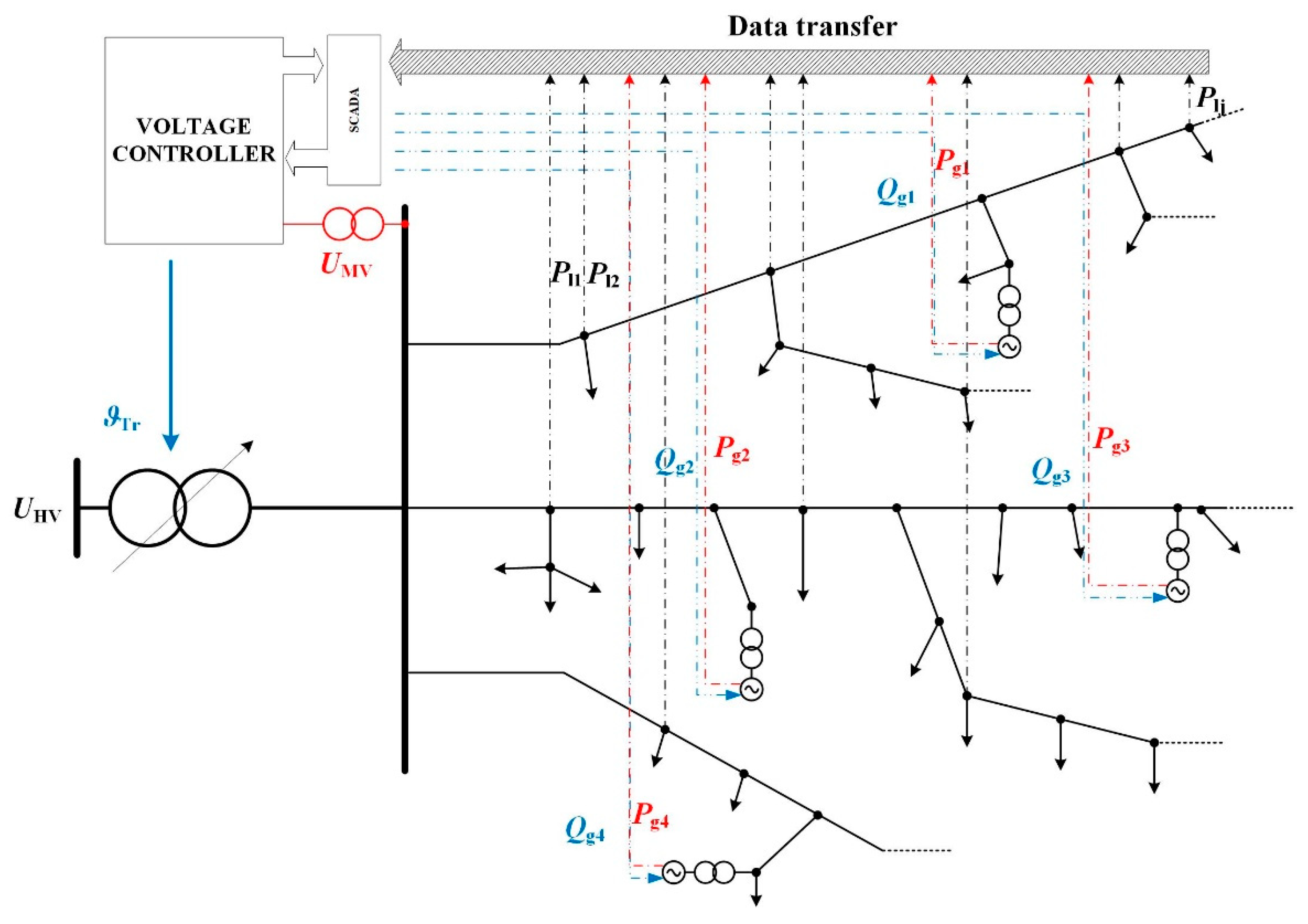
• two-criteria objective function—sum of the $F_1(x,y,z)$ function and modified $F_2(x,y,z)$ function with weighting factors $w_1,w_2$:

  $$F_3(x,y,z)=w_1\cdot F_1(x,y,z)+w_2\cdot F_{2\mathrm{M}}(x,y,z)=w_1\cdot F_1(x,y,z)+w_2\cdot \frac{\Delta P_{\mathrm{loss}}}{{\displaystyle \sum _{i=1}^m{P}_{\mathrm{L}i}}}$$

  (14)

  whereby:
  $x=\left[\vartheta , Q_{\mathrm{G}1}... Q_{\mathrm{G}k}... Q_{\mathrm{G}p}\right]$—vector of control variables formed by the transformer ratio ($\vartheta$–discrete variable) and reactive power of p sources connected to the MV network;
  $y=\left[U_{\mathrm{HV}}, P_{\mathrm{L}1}... P_{\mathrm{L}m},Q_{\mathrm{L}1}... Q_{\mathrm{L}m}, P_{\mathrm{G}1}... P_{Gp}\right]$—vector of independent variables, formed by: HV network supply voltage, active and reactive power received in m nodes, and power generated in p sources, not subject to change during optimization calculations;
  $z=\left[U_1... U_j, {\delta }_1... {\delta }_j\right]$—the vector of state variables containing nodal voltages and their arguments (total number of network nodes j = p + m).

The determination of the state vector z, for the known values of x and y vectors, is one of the basic computational problems included in the computer analysis of power systems. This problem, known as load flow analysis (LF), is described in textbooks such as [26,27].

Many algorithms and computer programs have been developed to solve this problem. Some of them are available as the Toolbox of the Matlab package (Matpower), but for the solutions provided in the proposed control system, they must be in the form of the dedicated ‘calculation engine’. Generally speaking, the components of the unknown vector z (state variables) are determined from a system of nonlinear equations of the form:

$$0=f_{\mathrm{LF}}(x,y,z)$$

(15)

Each equation is formulated for a node of the analyzed network so that the power balance for this node is equal to zero.

On the basis of nodal voltages (state variables), in view of the knowledge of the impedance parameters of the analyzed network, the power losses are determined based on the formula:

$$\Delta P_{\mathrm{loss}}={\displaystyle \sum _{(m,n)\in \left\{G\right\}}}{\left|\frac{U_m{e}^{\mathrm{j}{\delta }_m}- U_n{e}^{\mathrm{j}{\delta }_n}}{{\underset{\_}{Z}}_{mn}}\right|}^2\cdot R_{mn},$$

(16)

where m, n are terminal nodes of the network branch with impedance ${\underset{\_}{Z}}_{mn}=R_{mn}+\mathrm{j}{X}_{mn}$; all network branches form the set {G}.

Considering the above-described objective functions together with the vectors x, y, z, the optimization task can be formulated in the following way:

• objective function—the vector of control variables x providing the minimum function described (optionally) as (12), (13) or (14) is sought:

  $$F(x,y,z)\to \min$$

  (17)
• vector of inequality constraints h, ensuring that the elements of the vector of state variables and elements of the vector of control variables are kept within the range specified by the technical requirements:

  $$h\left(x,y,z\right)\ge 0$$

  (18)

Adopted as inequality restrictions were:

• minimum and maximum values for transformer ratio ($\vartheta$)

  $${\vartheta }_{\min }\le \vartheta \le {\vartheta }_{\max },$$

  (19)
• minimum and maximum reactive power values of each renewable source ($Q_{\mathrm{G}k}$)

  $$Q_{\mathrm{G}k}{}_{\min }\le Q_{\mathrm{G}k}\le Q_{\mathrm{G}k}{}_{\max },$$

  (20)
• minimum and maximum voltage values for all network nodes ($U_i$)

  $$U_{i\min }\le U_i\le U_i{}_{\max },$$

  (21)
• current-capacity limit values for power lines ($I_{l\max }$)

  $$I_l\le I_l{}_{\max }$$

  (22)
• the permissible load of the HV/MV transformer ($S_{\mathrm{nT}}$)

  $$S_{\mathrm{T}}\le S_{\mathrm{nT}}$$

  (23)

3.2. Description of the Heuristic Optimization Algorithm

After defining the objective function, one should choose the method of solving the optimization task. Over the past half-century, the optimal power flow has gained great attention due to its importance in the power system operation of HV grids [28,29,30]. Optimal power flow is considered an important tool for efficient planning and enhancing the operation of electric power systems. The main task of optimal power flow is to determine the best or the most secure operating point (control variables) of certain objective functions while satisfying the system equality and inequality constraints.

Given the small number of nodes in the distribution network and its simple (radial) structure, it is possible to apply real-time Optimal Power Flow (OPF) calculations into the voltage control concept, which is seen in Figure 1. In order to do so, it is necessary to create a network calculation model for each optimization cycle. This is possible thanks to the process of estimating its condition, which can be carried out thanks to measurements of voltage and power values—Figure 1. Further in this case, the radial structure and small size of the network allow this task to be performed in a much simpler mode than for multi-node meshed networks [31,32,33,34,35,36]. Being aware of the fundamental importance of the problem of network condition estimation for the effectiveness of the proposed voltage control solution, the authors decided to discuss this problem further in subsequent publications.

Several classical (deterministic) and recent (nondeterministic) heuristic optimization techniques have been proposed to find the solution to the optimal power flow problem. It should be pointed out that the classical methods may be trapped in a local optimum due to the nonlinearity of optimal power flow problems [37,38,39]; therefore, the metaheuristic optimization techniques are widely employed for solving the optimal power flow problems [38,40,41]. In part of the presented works, various heuristic methods were used to solve the optimization tasks [22,25,42,43,44]. Compared to classical methods, heuristic methods are characterized by the fact that they do not require knowledge of the derivative form of the objective function; they are resistant to discontinuities of this function and to ‘getting stuck’ in the calculation process at a local minimum. In the case of a divergent iterative process, data can be reloaded. The best solution recently found is not lost, as the solution vector is remembered at each stage of the calculation. The classical method would then have to be interrupted and the calculation restarted. The optimization method used in the research is called the Algorithm of the Innovative Gunner (AIG) [45]. It differs from more widely known heuristic methods [46,47,48], the way of generating new (successive) solutions. Generally speaking, in most heuristic methods (nearly 100 such methods are defined and described [37,49,50,51,52,53]), the iterative process of determining optimal values of the vector x components is similar, because most often, in the next iterative step, which can be considered as additive correction, the following action is performed:

$$x_l^{\left(i+1\right)}=x_l^{\left(i\right)}+\Delta x_l^{\left(i\right)}$$

(24)

and the correction of the l-th component of the vector, in the i-th iterative step, is determined as a function value:

$$\Delta x_l^{\left(i\right)}=f_l\left(\xi \right)$$

(25)

whereby function f_l and vector $\xi$ are characteristic of the heuristic method used [40,46,48].

In the case of the AIG algorithm, relation (24) is replaced by the expression:

$$x_l^{\left(i+1\right)}=x_l^{\left(i\right)}\cdot g_{l1}\left({\xi }_1\right)\cdot g_{l2}\left({\xi }_2\right)$$

(26)

Thus, the originality of the AIG method lies in the fact that in subsequent steps, the components of the x vector are changed by multiplying, not by adding. As functions $g_{l1}\left({\xi }_1\right), g_{l2}\left({\xi }_2\right)$, assuming that ${\xi }_1=\alpha , {\xi }_2=\beta$, the following ones are respectively adopted:

$$\begin{array}{l}g\left(\alpha \right)=\csc \left(\alpha \right)={\left(\cos \left(\alpha \right)\right)}^{-1} \mathrm{for} \alpha >0\\ g\left(\alpha \right)=\cos \left(\alpha \right) \mathrm{for} \alpha <0\\ g\left(\beta \right)=\csc \left(\beta \right)={\left(\cos \left(\beta \right)\right)}^{-1} \mathrm{for} \beta >0\\ g\left(\beta \right)=\cos \left(\beta \right) \mathrm{for} \beta <0\end{array}$$

(27)

where α and β are ‘correction angles’, drawn from a range $\left(-{\alpha }_{\max },{\alpha }_{\max }\right) \mathrm{and} \left(-{\beta }_{\max },{\beta }_{\max }\right)$ using a normal or uniform probability distribution. The process of solving optimization tasks for the objective function and the vector of decision variables x is as follows [45]:

• drawing of initial values of the components of the decision vector x₀,
• finding the objective function F value for the start vector x₀,
• setting the iteration counter to t = 1,
• determining the scope of ${\alpha }_{\max }$ and ${\beta }_{\max }$,
• correction of the decision vector x components by means of multiplicative correction factors g(α), g(β),
• determination of a new state of the analyzed system (in the case of the OPF task, solution of the system of Equation (15)),
• determining the value of objective function F for subsequent solutions, checking if the objective function for the next solution is better than the solution from the previous iteration (if so, replace this solution with the current—better—solution, and if not—leave it), identification of the q solution for which the function reaches the minimum value,
• checking whether for the identified solution q, the relation $F\left({\mathit{x}}_q^{i+1}\right)<F_{\mathrm{best}}\left({\mathit{x}}_{\mathrm{best}}^i\right)$ occurs; if so, then accepting it as the next decision vector in the iterative process, i.e., ${\mathit{x}}_{\mathrm{best}}^{i+1}={\mathit{x}}_q^{i+1}$
• verification of the stopping criterion (t + 1 = t_max), end or subsequent iteration (t = t + 1), and return to point d,
• end of calculation.

Considering a population of new solutions in the AIG algorithm, it is characterized by a large exploration of the search space. The subsequent solutions differ (sometimes quite significantly) from the previous ones, which allows the avoiding of the local optimum. The effectiveness of the AIG algorithm has been confirmed for many test tasks in the area of mathematics and technology [45]. In power engineering applications (also OPF, [41]), the AIG algorithm works on the basis of an autonomous ‘calculation engine’, performing load flow (LF) calculations in subsequent steps.

The authors wish to emphasize that the use of the AIG algorithm results from the fact it was invented by them, and new confirmations are sought that, despite its simplicity, it can be effectively applied in many optimization tasks. In order to confirm the correctness of the obtained results, calculations were also carried out with the use of the CS (Cuckoo Search [48]) algorithm, one of the best-known metaheuristic algorithms.

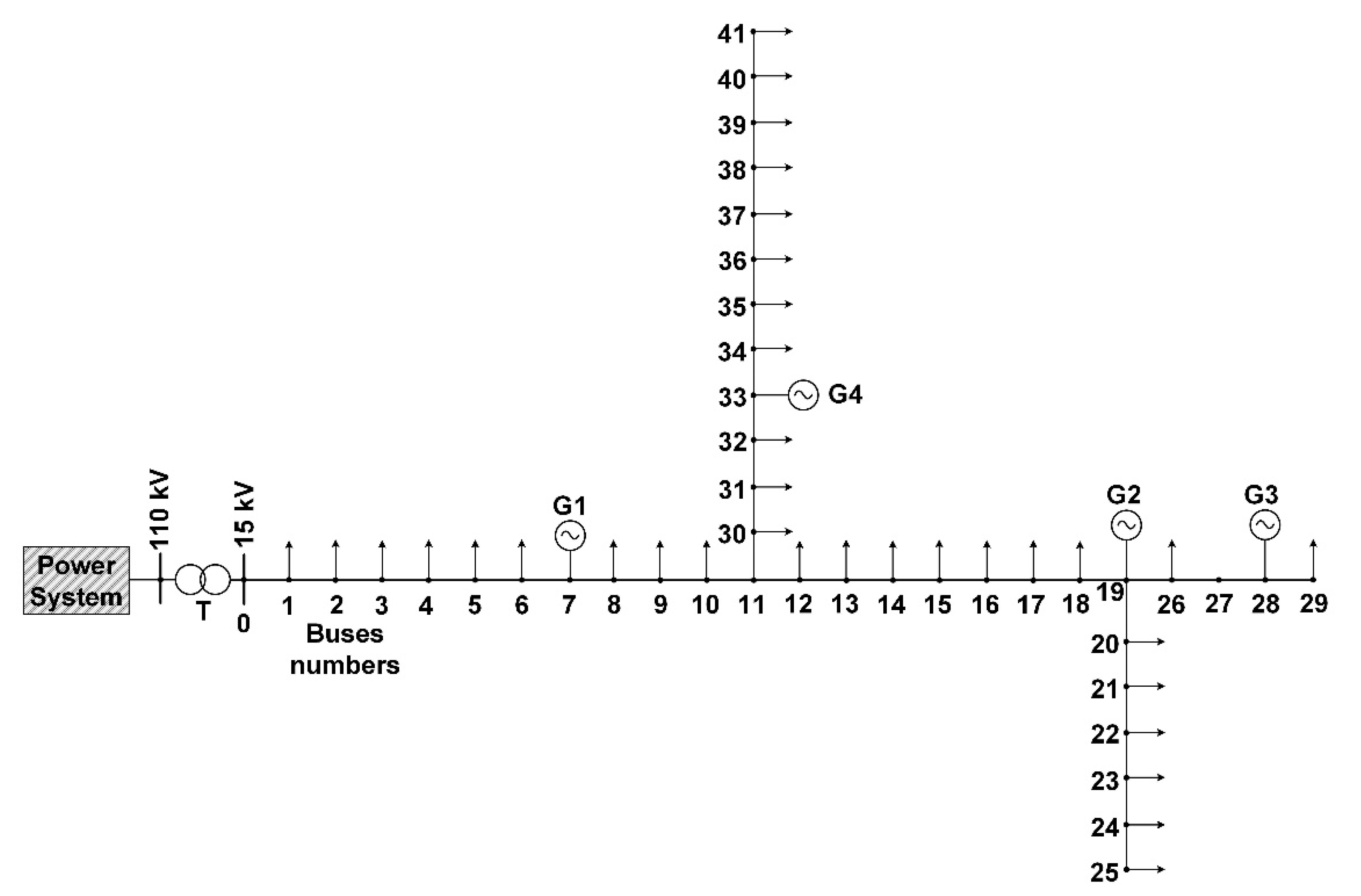
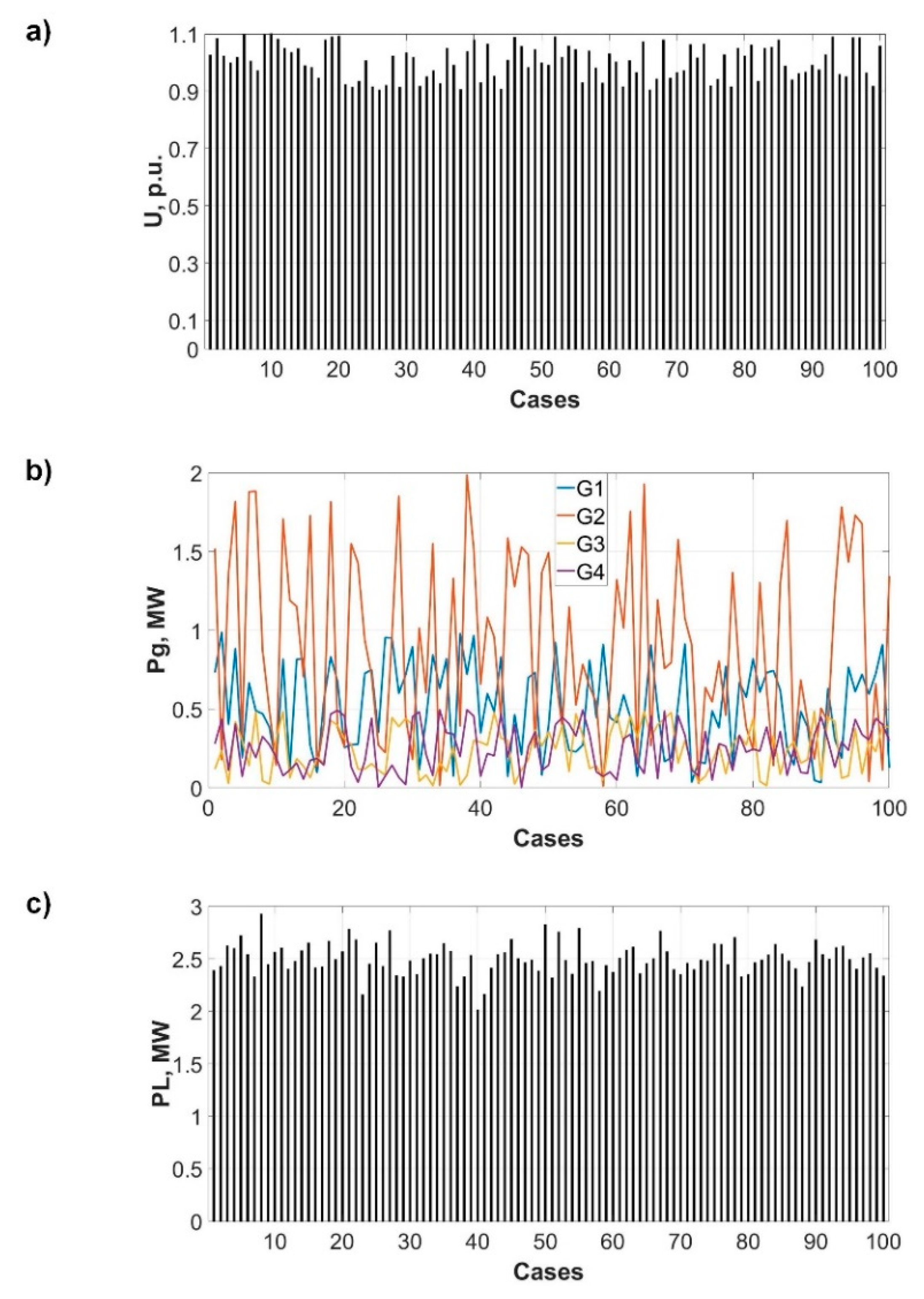
4. Description of the Test Network and Methodology of the Tests Carried Out

In order to verify the effectiveness of the proposed voltage regulation concept, a multi-variant test calculation was performed. For the analyses, a network model consisting of a 15 kV overhead power line with branches, with a total length of 33.5 km, made with ACSR 70 mm² conductors, was used. It corresponds to the actual line located in the central part of Poland in Figure 2. There is a transformer with a power of 10 MVA and a ratio ϑ = 115/16.5 kV/kV ± 10% (taps every 1.11%). Four sources with rated capacities of P_nG1 = 1 MW, P_nG2 = 2 MW, P_nG3 = 0.5 MW, and P_nG4 = 0.5 MW are connected to the network. Each source has the capacity to generate reactive power in the range $\left(-0.4, 0.4\right)P_{\mathrm{nG}}$, and this power is remotely controlled in the system proposed in Figure 1.

The network load includes MV/LV transformer substations connected in almost all nodes (the total number of nodes is m = 42), except for nodes with the numbers 0, 7, 11, 19, 27, 28, and 33 (Figure 2). The maximum loads of individual nodes are shown in Figure 3.

A single solution to the optimization task would not allow us to draw reliable conclusions about the effectiveness of the proposed voltage control system using the HV/MV transformer tap changer and reactive power of generators connected to the MV network. That is why the search for the solution was repeated many times—in the initial stage, the number was one hundred. The values of the control variables were drawn by means of a random number generator with a rectangular distribution, from the following ranges:

U_HV voltage from the range $\left(0.9, 1.1\right)U_{\mathrm{nHV}}$

• load at the node i $\left(\frac{1}{3}, 1\right)P_{\mathrm{Lmax}i}$
• generation in node k including $\left(\frac{1}{3}, 1\right)P_{\mathrm{nG}k}$

Figure 4a shows the selected values of U_HV voltage for a cycle of 100 draws, Figure 4b shows the drawn values of the power generated in sources, and Figure 4c shows the total value of the power received in the receiving nodes resulting from draws. In the case of the receiving nodes, the random load of reactive power determined by the coefficient tgϕ = 0.4 was also modeled.

There is no correlation between the drawn values of U_HV voltage, loads in nodes, and active power generated in sources. These values do not represent a specific time of day or weather condition. The intention of the authors was to check the effectiveness of optimization calculations for a large number of completely random independent variable values. The results of these analyses should be regarded as positive.

5. Results of Single-Criteria Optimization

5.1. The Way of Presenting the Research Results

In order to justify the effectiveness of the proposed method of voltage control in the MV network, the results of the optimization process repeated for 100 calculation cycles were presented. For each of them, a set of independent variables (y vector) was randomly generated. In order to justify the final choice of the objective function, the effects of the six considered methods of control have been compared graphically below:

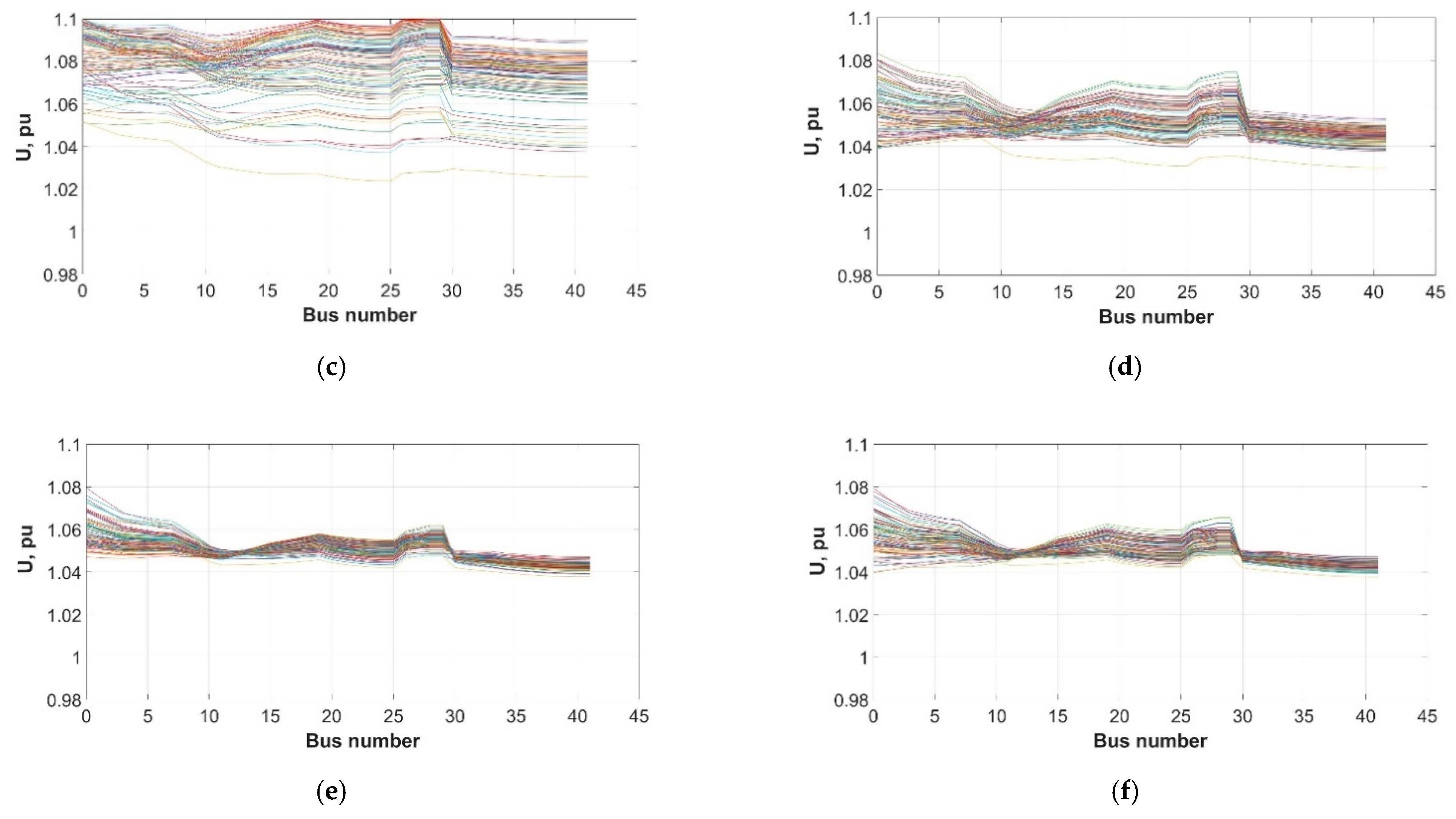
• the effects of traditional control, i.e., maintaining a constant voltage value of 1.05 U_nMV, on the MV busbars, using OLTC;
• control effects, the aim of which is to minimize the single-criterion objective function (12), i.e., to minimize the square of the relative voltage deviations from the value of 1.05 U_nMV determined for all network nodes, using OLTC and appropriately selected reactive power values of distributed sources, as for all the next cases;
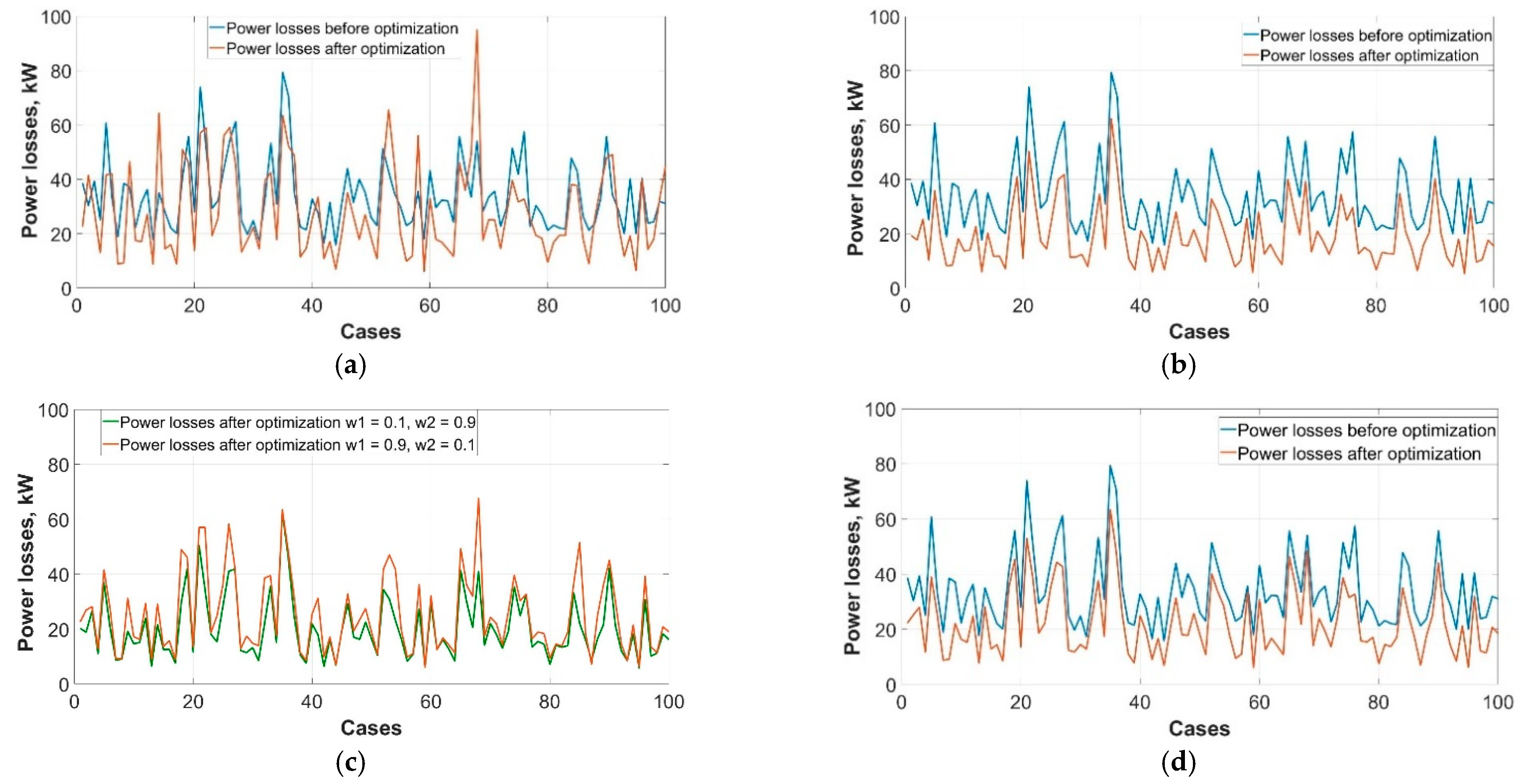
• effects of regulation, the aim of which is to minimize the single-criteria objective function (13), i.e., to minimize power losses in the MV grid;
• the effects of minimizing the two-criteria objective function (15), where the voltage deviation component has the weighting factor w1 = 0.1, and the relative power loss indicator w2 = 0.9;
• the effects of minimizing the two-criteria objective function (15), where the voltage deviation component has the weighting factor w1 = 0.9, and the relative power loss indicator w2 = 0.1;
• the effects of minimizing the two-criteria objective function (15), where the voltage deviation component has the weighting factor w1 = 0.7, and the relative power loss indicator w2 = 0.3.

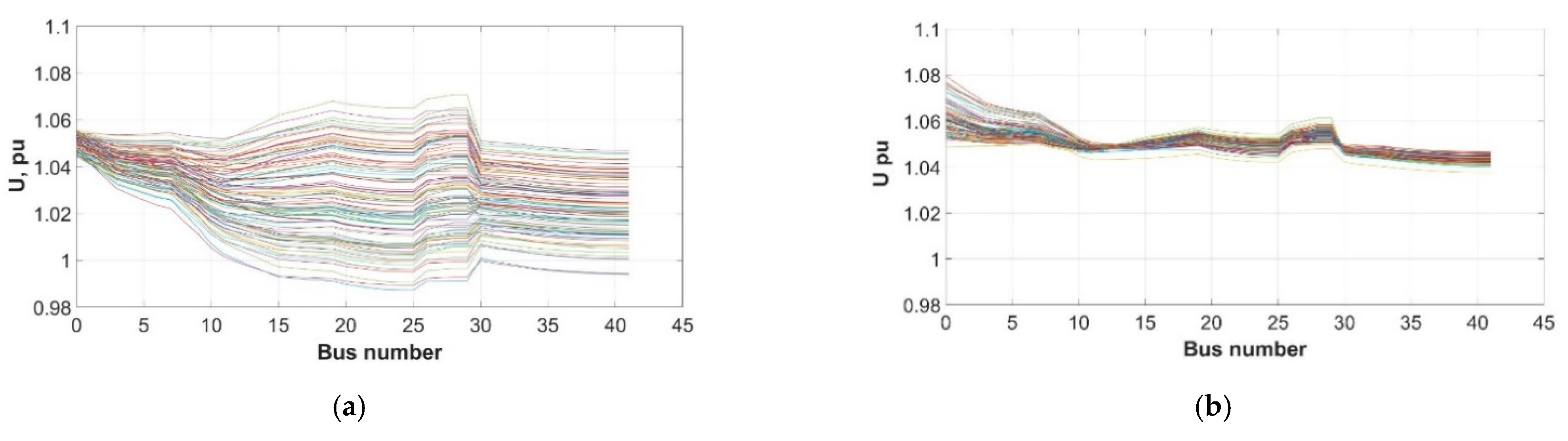
5.2. Qualitative Assessment of Voltage Control

Figure 5 shows the voltage values for all network nodes, obtained for all 100 calculation cycles. The charts form characteristic ‘bands’ that are used for the qualitative assessment of the effects of control. The larger the band area, the worse the concentration of the voltages around 1.05 U_nMV is, and therefore, the control is less effective. Undoubtedly, the greatest approximation of the voltage value to the expected value 1.05 U_nMV is shown in Figure 5b,e for which the voltage criterion has the only or dominant significance. Minimizing the power losses (Figure 5c,d) noticeably worsens the voltage quality. For the two-criteria optimization and the weighting factors w1 = 0.7 and w2 = 0.3, the band area slightly widens, compared to the single-criteria optimization according to (12).

5.3. Quantitative Assessment of Voltage Control

The qualitative evaluation of the voltage for various control methods was supplemented with the quantitative evaluation with the use of the indicator value (12), as shown in Figure 6. The results for the OLTC regulation case, shown in Figure 6a,b,d (blue), were taken as reference. The average value of the indicator (for all calculation cycles) was F_1av = 0.0262, while the worst value was F₁ = 0.1052. Optimization according to function (12)—Figure 6a—reduces the value of the voltage quality indicator so dramatically that while keeping the y-axis scale the same as for the traditional regulation, its values obtained for the subsequent calculation cycles are almost invisible. The worst case is F₁ = 0.0037, mean value F_1av = 0.0010—about 26 times less than in the case of the traditional solution. Minimizing power losses causes a very slight reduction in the voltage quality indicator (Figure 6b). The same indicator is very sensitive to the optimization process, because even with the weighting factor w1 = 0.1, its value significantly improves compared to the reference value (Figure 6c). For the weighting factor w1 = 0.3, the two-criteria optimization is almost as effective as for the single-criteria approach (12) (Figure 6d).

5.4. Power Losses, Selection of Weighting Factors

Good voltage quality, although justified from the consumers’ point of view, does not significantly reduce the value of power losses. This is due to the fact that reactive power is used in the control process, which increases the value of losses. This is shown in Figure 7. For the traditional control, the mean losses ∆P_loss = 34.1 kW, and after optimization (according to voltage quality index), it changed very slightly to ∆P_loss = 28.6 kW—Figure 7a. On the other hand, the value of the objective function (level of power losses) has clearly decreased—Figure 7b. The average value of F₂ (power losses (13)) after optimization decreased significantly, to ∆P_loss = 19.3 kW.

The analyses carried out for the one-criteria objective functions F₁ and F₂ indicate that effective optimization of the voltage indicator does not decrease power losses, and minimizing losses has a negative impact on the value of the voltage indicator. Therefore, an attempt to apply polyoptimization is justified, according to the proposed function (15). The question of selecting the w1, w2 weighting factors remains. Below,

Table 1. Summary of results of two-criteria optimization (15) for different weighting factors (w1—responsible for voltage quality, w2—responsible for power losses), one hundred calculation cycles.

Weight w1	Weight w2	Voltage Indicator F1max	Voltage Indicator F1av	Power Losses ΔPloss_max [kW]	Power Losses ΔPloss_av [kW]
0.1	0.9	0.0094	0.0024	62.5	20.2
0.3	0.7	0.0051	0.0018	62.7	20.6
0.5	0.5	0.0040	0.0015	63.0	21.2
0.7	0.3	0.0038	0.0013	63.5	22.3
0.9	0.1	0.0037	0.0011	67.7	25.2

presents the results of two-criteria optimization for five pairs of these factors.

As expected, the use of a pair of weighting factors (w1 = 0.1, w2 = 0.9) gives better results in reducing power losses than (w1 = 0.9, w2 = 0.1)—Figure 7c. Both Table 1 and Figure 5f, Figure 6d and Figure 7d confirm that the selection of the weighting factors (w1 = 0.7, w2 = 0.3) gives both a significant reduction in the voltage quality indicator and a reduction in power losses by an average of 40%, hence the authors’ recommendation for these factor values.

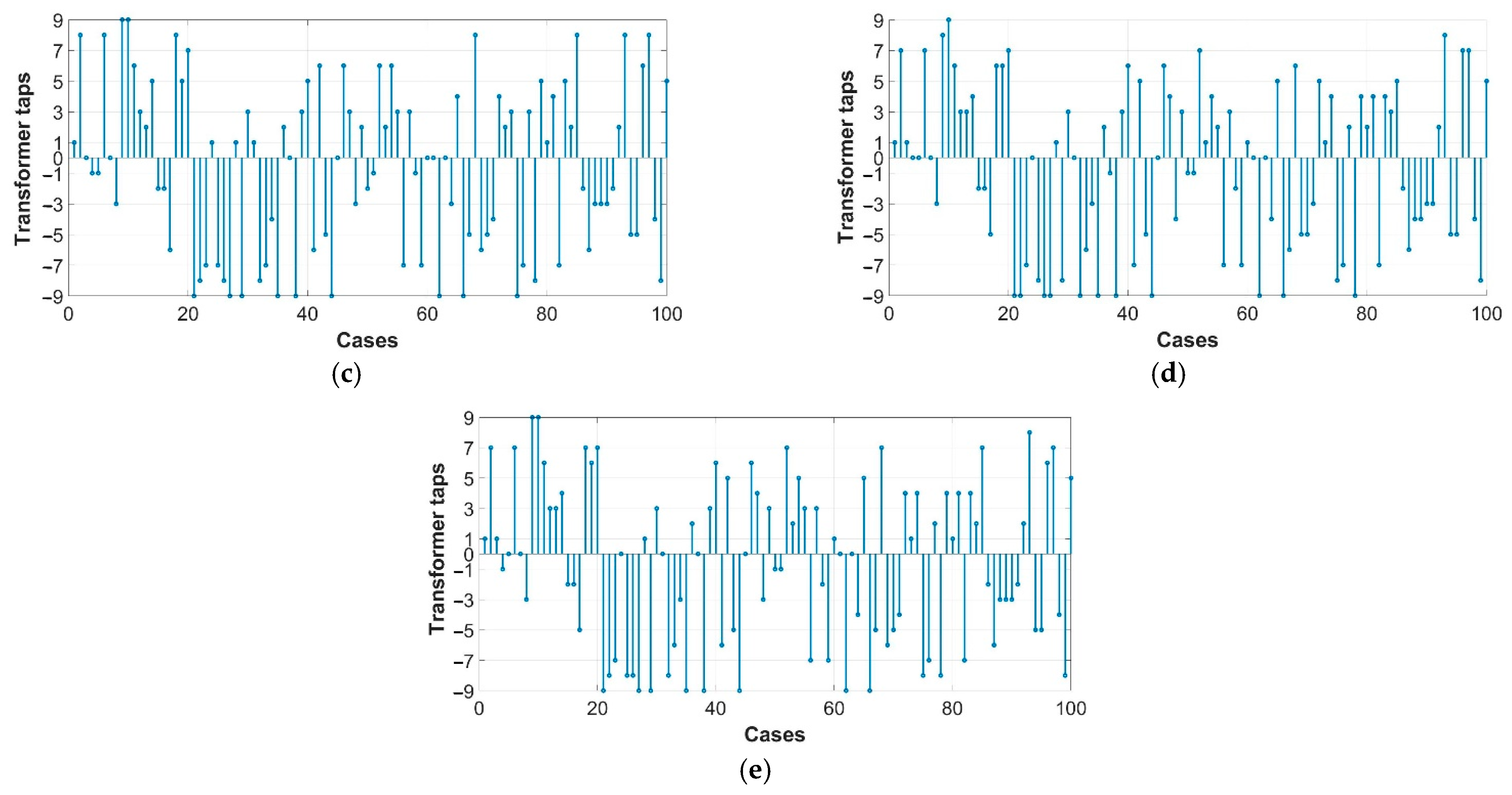
5.5. The Values of Decision Variables

The following figures show the values of the decision variables (vector x) occurring in successive variants of the optimal voltage control process. Figure 8 shows the tap changer numbers of the OLTC determined for voltage quality optimization (a), power loss minimization (b), and two-criteria optimization for the three pairs of weighting factors (c, d, f) listed in Table 1. Figure 9 shows the values of the reactive power of the G1, G2, G3, G4 generators corresponding to the above-mentioned optimization processes. It is difficult to formulate general conclusions based on the qualitative observation of changes in the presented values, but it can be noticed that the optimization process adjusts the voltage values to the form of the objective function. Thus, it is not justified to make simplified statements that distributed sources overestimate the voltage values in the network; these voltages vary within wide limits, and only the comprehensive interaction of control variables effectively reduces this variability and equalizes the voltage in the entire network.

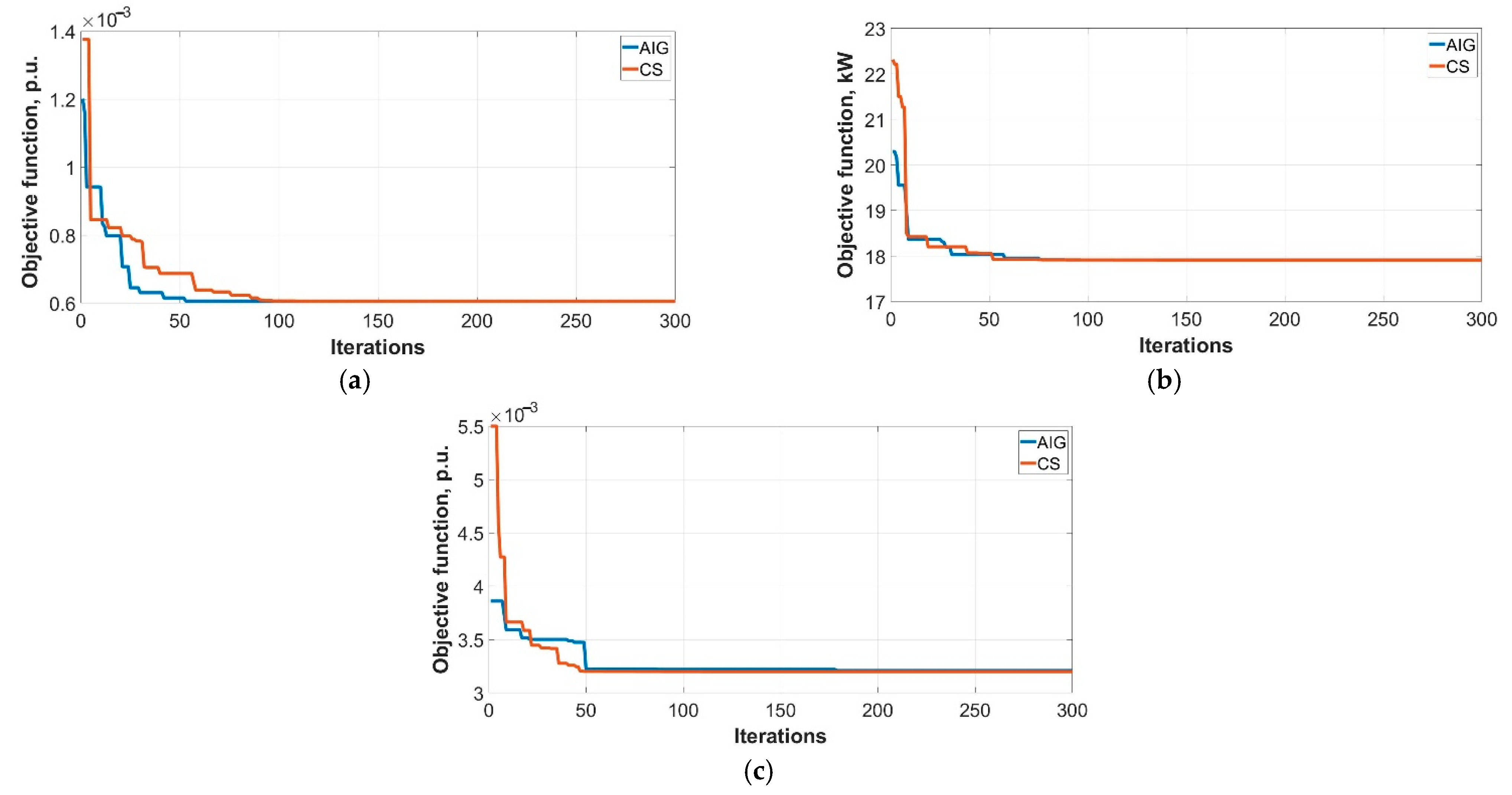
5.6. The Effectiveness of the AIG Optimization Algorithm and Verification of the Calculation Results

In order to verify the correctness of the proprietary AIG algorithm, analogous calculations were performed according to the very popular metaheuristic algorithm—Cuckoo Search (CS). The results are shown in Figure 10 and in

Table 2. The optimal voltage values in network nodes for two heuristic algorithms (AIG and CS) and three objective functions, for one of the calculation cycles.

Bus No.	The Load Power, PL, kW	Voltage before Optimization, U p.u.	Voltage after Optimization, U p.u.
			Objective Function F1		Objective Function F2		Objective Function F3 w1 = 0.7, w2 = 0.3
			AIG	CS	AIG	CS	AIG	CS
0	0	1.0497	1.0533	1.0533	1.0811	1.0811	1.0453	1.0453
1	45.29	1.0480	1.0524	1.0524	1.0813	1.0813	1.0451	1.0452
2	15.57	1.0465	1.0517	1.0517	1.0816	1.0816	1.0451	1.0451
3	320.65	1.0450	1.0509	1.0509	1.0820	1.0820	1.0450	1.0451
4	39.46	1.0447	1.0511	1.0510	1.0826	1.0826	1.0455	1.0456
5	87.43	1.0445	1.0512	1.0512	1.0833	1.0833	1.0460	1.0461
6	26.01	1.0444	1.0515	1.0515	1.0841	1.0841	1.0467	1.0468
7	0.00	1.0444	1.0517	1.0517	1.0846	1.0846	1.0471	1.0472
8	232.60	1.0424	1.0499	1.0499	1.0840	1.0841	1.0461	1.0462
9	46.23	1.0413	1.0489	1.0489	1.0844	1.0844	1.0460	1.0461
10	80.95	1.0401	1.0479	1.0478	1.0848	1.0849	1.0460	1.0461
11	0.00	1.0395	1.0474	1.0474	1.0854	1.0854	1.0462	1.0463
12	24.86	1.0408	1.0484	1.0484	1.0876	1.0876	1.0480	1.0482
13	46.22	1.0422	1.0495	1.0495	1.0898	1.0899	1.0499	1.0501
14	48.24	1.0437	1.0507	1.0507	1.0922	1.0922	1.0520	1.0522
15	170.92	1.0453	1.0520	1.0520	1.0947	1.0947	1.0541	1.0543
16	35.83	1.0462	1.0528	1.0527	1.0959	1.0959	1.0552	1.0554
17	47.79	1.0471	1.0536	1.0535	1.0972	1.0972	1.0563	1.0566
18	58.01	1.0481	1.0544	1.0544	1.0985	1.0986	1.0576	1.0578
19	0.00	1.0491	1.0553	1.0553	1.0999	1.1000	1.0588	1.0590
20	202.48	1.0476	1.0538	1.0537	1.0985	1.0985	1.0573	1.0575
21	41.21	1.0467	1.0529	1.0529	1.0976	1.0977	1.0564	1.0567
22	37.82	1.0460	1.0522	1.0522	1.0970	1.0970	1.0557	1.0560
23	120.94	1.0454	1.0516	1.0516	1.0964	1.0964	1.0552	1.0554
24	31.04	1.0452	1.0515	1.0514	1.0962	1.0963	1.0550	1.0552
25	23.10	1.0452	1.0514	1.0514	1.0962	1.0962	1.0549	1.0552
26	24.76	1.0490	1.0546	1.0545	1.0998	1.0999	1.0583	1.0585
27	0.00	1.0490	1.0540	1.0539	1.0999	1.1000	1.0580	1.0581
28	0.00	1.0491	1.0538	1.0537	1.0999	1.1000	1.0578	1.0580
29	50.05	1.0491	1.0538	1.0537	1.0999	1.1000	1.0578	1.0580
30	181.07	1.0384	1.0465	1.0465	1.0846	1.0846	1.0453	1.0455
31	222.54	1.0377	1.0460	1.0460	1.0840	1.0841	1.0448	1.0449
32	20.94	1.0374	1.0459	1.0459	1.0839	1.0840	1.0446	1.0448
33	0.00	1.0371	1.0458	1.0458	1.0839	1.0839	1.0446	1.0447
34	214.51	1.0362	1.0450	1.0449	1.0830	1.0831	1.0437	1.0439
35	52.57	1.0357	1.0444	1.0444	1.0825	1.0826	1.0432	1.0434
36	57.17	1.0352	1.0440	1.0439	1.0821	1.0821	1.0427	1.0429
37	41.80	1.0348	1.0436	1.0436	1.0817	1.0817	1.0423	1.0425
38	66.96	1.0345	1.0433	1.0432	1.0814	1.0814	1.0420	1.0422
39	51.10	1.0343	1.0431	1.0430	1.0812	1.0812	1.0418	1.0420
40	21.71	1.0342	1.0429	1.0429	1.0811	1.0811	1.0417	1.0419
41	56.69	1.0341	1.0429	1.0428	1.0810	1.0810	1.0416	1.0418

,

Table 3. The optimal values of reactive power of sources for two heuristic algorithms, for one of the calculation cycles.

Gen No.	Power Generation, PG, MW	Reactive Power Generated as a Result of the Optimization, Q, M Var
		Objective Function F1		Objective Function F2		Objective Function F3 w1 = 0.7, w2 = 0.3
		AIG	CS	AIG	CS	AIG	CS
G1	0.815	0.400	0.400	0.400	0.400	0.400	0.400
G2	1.812	0.062	0.061	0.482	0.472	0.395	0.410
G3	0.064	−0.200	−0.200	0.000	0.010	−0.124	−0.134
G4	0.457	0.200	0.200	0.200	0.200	0.200	0.200

and

Table 4. The optimal values of tap changer position and objective function for two heuristic algorithms, for one of the calculation cycles.

Objective Function	Tap Changer Position		The Value of the Objective Function
	AIG	CS	AIG	CS
F1	4	4	0.000606 pu	0.000606 pu
F2	2	2	17.914 kW	17.912 kW
F3 (w1 = 0.7, w2 = 0.3)	5	5	0.0032 pu	0.0032 pu

. In all cases, the optimization process is very fast; about 50 iterations lead practically to the minimum value of the objective function.

Below, Table 2 presents the optimal voltage values in network nodes for two heuristic algorithms (AIG and CS) and three objective functions, for one of the calculation cycles. The table also includes the voltage values before optimization and the load power. The random voltage value on the HV side was U_HV = 1.0514 p.u.

Below, Table 3 presents the optimal values of the reactive power of sources for two heuristic algorithms (AIG and CS) and three objective functions for one sample of the calculation cycles (the same as in Table 2).

Table 4 contains the optimal values of the HV/MV transformer tap changer and optimal value of the objective function, for two heuristic algorithms (AIG and CS) and three objective functions for one sample of the calculation cycles (the same as in Table 2 and Table 3).

Full compliance of the results obtained with the proprietary AIG algorithm and the well-known CS algorithm, with a noticeably better convergence and speed of AIG, confirms its good properties demonstrated in other applications.

6. Discussion and Conclusions

The voltage control system proposed in Figure 1 for MV networks with distributed sources allows the achievement of favorable voltage level, both in terms of values and in terms of minimizing power losses. This is possible through the traditional application of the on-load tap changer of the HV/MV transformer and the innovative, appropriate use of the reactive power control capabilities of distributed sources. The key to achieving a control quality significantly better than that of traditional fixed-value control is the use of an algorithm to minimize the objective function, with the best results being achieved through a two-component function-based polyoptimization (14).

The concept presented contains a number of assumptions simplifying and idealizing the optimization process, performed as a heuristic optimization using the proprietary AIG algorithm. This process can take place provided that the network model is properly estimated and iterative load flow calculations, which are an essential element of the OPF algorithm, are performed on it. This issue was not discussed in detail in the article, but the technological development of network data transmission and processing systems makes it possible to look realistically at obtaining such possibilities on-line at the control system level. The concept is realistic because the dimension of the calculation task is small, and there are no particularly high requirements in view of the speed of the control process. In this way, the characteristics of smart grids will be achieved. It will be possible to introduce such operation at the MV level as the answer of control variables to the load changes and generation variability of distributed sources.

References

1. Farkas, C.; Tóth, A.; Orlay, I. Voltage Control Methods in the MV Grid with a Large Share of PV. Int. J. Emerg. Electr. Power Syst. 2019, 20. [Google Scholar] [CrossRef]
2. Sigalo, M.B.; Eze, K.; Usman, R. Analysis of medium and low voltage distribution network with high level penetration of distributed generators using eracs. Eur. J. Eng. Technol. 2016, 4, 9–23. [Google Scholar]
3. Zhang, D.; Li, J.; Hui, D. Coordinated control for voltage regulation of distribution network voltage regulation by distributed energy storage systems. Prot. Control Mod. Power Syst. 2018, 3. [Google Scholar] [CrossRef]
4. Pijarski, P.; Kacejko, P.; Adamek, S. Analysis of Voltage Conditions in Low Voltage Networks Highly Saturated with Photovoltaic Micro Installations. Acta Energ. 2018, 2018, 4–9. [Google Scholar] [CrossRef]
5. Kazmi, S.; Shahzad, M.; Shin, D. Multi-Objective Planning Techniques in Distribution Networks: A Composite Review. Energies 2017, 10, 208. [Google Scholar] [CrossRef] [Green Version]
6. Mahmud, N.; Zahedi, A. Review of control strategies for voltage regulation of the smart distribution network with high penetration of renewable distributed generation. Renew. Sust. Energy Rev. 2016, 64, 582–595. [Google Scholar] [CrossRef]
7. Iman, Z. Planning of Distribution Networks for Medium Voltage and Low Voltage. Ph.D. Thesis, Queensland University of Technology, Queensland, Australia, 2011. [Google Scholar]
8. Kacejko, P.; Pijarski, P. Zarządzanie mikroinstalacjami OZE—realne wyzwanie techniczne, czy tylko impuls marketingowy? [Mangement of microgenerations of renewable energy sources—technical chalange or the marketing impuls?]. Rynek Energii 2016, 2016, 41–45. [Google Scholar]
9. EN 50160: Voltage Characteristics of Electricity Supplied by Public Distribution Network; PKN: Warsaw, Poland, 2019.
10. IEC. IEC 60038: IEC Standard Voltages; International Electrotechnical Commission (IEC): Geneva, Switzerland, 2009. [Google Scholar]
11. Kot, A. Optimal Voltage Control in Medium Voltage Distribution Networks with Dispersed Generation. Ph.D. Thesis, AGH University of Science and Technology, Cracow, Poland, 2005. [Google Scholar]
12. Szpyra, W.; Kot, A. Optimal voltage control in medium voltage power distribution networks. Acta Energ. 2009, 2, 89–105. [Google Scholar]
13. Agalgaonkar, Y.; Pal, B.C.; Jabr, R.A. Distribution voltage control considering the impact of PV generation on tap changers and autonomous regulators. In Proceedings of the 2014 IEEE PES General Meeting | Conference & Exposition. 2014 IEEE Power & Energy Society General Meeting, National Harbor, MD, USA, 27–31 July 2014; p. 1, ISBN 978-1-4799-6415-4. [Google Scholar]
14. Neagu, B.C.; Grigoras, G. Optimal Voltage Control in Power Distribution Networks Using an Adaptive On-Load Tap Changer Transformers Techniques. In Proceedings of the 2019 International Conference on Electromechanical and Energy Systems (SIELMEN). 2019 International Conference on Electromechanical and Energy Systems (SIELMEN), Craiova, Romania, 9–11 October 2019; pp. 1–6, ISBN 978-1-7281-4011-7. [Google Scholar]
15. Adamek, S. Optimal Voltage Control in Distributed Power Grid with Dispersed Generation. Ph.D. Thesis, Lublin University of Technology, Lublin, Poland, 2010. [Google Scholar]
16. Kacejko, P.; Adamek, S.; Wydra, M. Optimal voltage control in distribution networks with dispersed generation. In Proceedings of the 2010 IEEE PES Innovative Smart Grid Technologies Conference Europe (ISGT Europe). 2010 IEEE PES Innovative Smart Grid Technologies Conference Europe (ISGT Europe), Gothenburg, Sweden, 11–13 October 2010; pp. 1–4, ISBN 978-1-4244-8508-6. [Google Scholar]
17. Dib, M.; Ramzi, M.; Nejmi, A. Voltage regulation in the medium voltage distribution grid in the presence of renewable energy sources. Mater. Today Proc. 2019, 13, 739–745. [Google Scholar] [CrossRef]
18. Guo, Y.; Wu, Q.; Gao, H.; Shen, F. Distributed voltage regulation of smart distribution networks: Consensus-based information synchronization and distributed model predictive control scheme. Int. J. Electr. Power Energy Syst. 2019, 111, 58–65. [Google Scholar] [CrossRef]
19. Agalgaonkar, Y.P.; Pal, B.C.; Jabr, R.A. Distribution Voltage Control Considering the Impact of PV Generation on Tap Changers and Autonomous Regulators. IEEE Trans. Power Syst. 2014, 29, 182–192. [Google Scholar] [CrossRef] [Green Version]
20. Castro, J.R.; Saad, M.; Lefebvre, S.; Asber, D.; Lenoir, L. Optimal voltage control in distribution network in the presence of DGs. Int. J. Electr. Power Energy Syst. 2016, 78, 239–247. [Google Scholar] [CrossRef]
21. Lu, J.; Wang, B.; Ren, H.; Zhao, D.; Wang, F.; Shafie-khah, M.; Catalão, J. Two-Tier Reactive Power and Voltage Control Strategy Based on ARMA Renewable Power Forecasting Models. Energies 2017, 10, 1518. [Google Scholar] [CrossRef] [Green Version]
22. Bedawy, A.; Yorino, N.; Mahmoud, K.; Zoka, Y.; Sasaki, Y. Optimal Voltage Control Strategy for Voltage Regulators in Active Unbalanced Distribution Systems Using Multi-Agents. IEEE Trans. Power Syst. 2020, 35, 1023–1035. [Google Scholar] [CrossRef]
23. Kryonidis, G.C.; Demoulias, C.S.; Papagiannis, G.K. A new voltage control scheme for active medium-voltage (MV) networks. Electr. Power Syst. Res. 2019, 169, 53–64. [Google Scholar] [CrossRef]
24. Wlodarczyk, P.; Sumper, A.; Cruz, M. Voltage Control of Distribution Grids with Multi-Microgrids Using Reactive Power Management. AECE 2015, 15, 83–88. [Google Scholar] [CrossRef]
25. Tengku Hashim, T.J.; Mohamed, A. Optimal coordinated voltage control in active distribution networks using backtracking search algorithm. PLoS ONE 2017, 12, e0177507. [Google Scholar] [CrossRef] [Green Version]
26. Salam, M.A. Fundamentals of Electrical Power Systems Analysis; Springer: Singapore, MI, USA, 2020; ISBN 978-981-15-3211-5. [Google Scholar]
27. Murty, P.S.R. Power Systems Analysis; Elsevier Science: Saint Louis, MO, USA, 2017; ISBN 9780081011119. [Google Scholar]
28. Frank, S.; Steponavice, I.; Rebennack, S. Optimal power flow: A bibliographic survey I. Energy Syst 2012, 3, 221–258. [Google Scholar] [CrossRef]
29. Dommel, H.; Tinney, W. Optimal Power Flow Solutions. IEEE Trans. Power Appar. Syst. 1968, PAS-87, 1866–1876. [Google Scholar] [CrossRef]
30. Lin, J.; Magnago, F.H. Optimal Power Flow. In Electricity Markets: Theories and Applications; John Wiley & Sons, Inc.: Hoboken, NJ, USA, 2017; pp. 141–171. ISBN 9781119179382. [Google Scholar]
31. Petinrin, J.O.; Shaabanb, M. Impact of renewable generation on voltage control in distribution systems. Renew. Sustain. Energy Rev. 2016, 65, 770–783. [Google Scholar] [CrossRef]
32. Sharma, V.; Aziz, S.M.; Haque, M.H.; Kauschke, T. Effects of high solar photovoltaic penetration on distribution feeders and the economic impact. Renew. Sustain. Energy Rev. 2020, 131, 110021. [Google Scholar] [CrossRef]
33. Sarimuthu, C.R.; Ramachandaramurthy, V.K.; Agileswari, K.R.; Mokhlis, H. A review on voltage control methods using on-load tap changer transformers for networks with renewable energy sources. Renew. Sustain. Energy Rev. 2016, 62, 1154–1161. [Google Scholar] [CrossRef]
34. Oh, C.-H.; Go, S.-I.; Choi, J.-H.; Ahn, S.-J.; Yun, S.-Y. Voltage Estimation Method for Power Distribution Networks Using High-Precision Measurements. Energies 2020, 13, 2385. [Google Scholar] [CrossRef]
35. Mohagheghi, E.; Alramlawi, M.; Gabash, A.; Li, P. A Survey of Real-Time Optimal Power Flow. Energies 2018, 11, 3142. [Google Scholar] [CrossRef] [Green Version]
36. Dzafic, I.; Ablakovic, D.; Henselmeyer, S. Real-time three-phase state estimation for radial distribution networks. In Proceedings of the 2012 IEEE Power and Energy Society General Meeting. 2012 IEEE Power & Energy Society General Meeting. New Energy Horizons–Opportunities and Challenges, San Diego, CA, USA, 22–26 July 2012; pp. 1–9, ISBN 978-1-4673-2729-9. [Google Scholar]
37. Zhu, J. Optimization of Power System Operation; John Wiley & Sons, Inc.: Hoboken, NJ, USA, 2015; ISBN 9781118887004. [Google Scholar]
38. Ebeed, M.; Kamel, S.; Jurado, F. Optimal Power Flow Using Recent Optimization Techniques. Classical and Recent Aspects of Power System Optimization; Elsevier: New York, NY, USA, 2018; pp. 157–183. ISBN 9780128124413. [Google Scholar]
39. Glavitsch, H.; Bacher, R. Optimal Power Flow Algorithms. Analysis and Control System Techniques for Electric Power Systems, Part 1 of 4; Elsevier: New York, NY, USA, 1991; pp. 135–205. ISBN 9780120127412. [Google Scholar]
40. Mirjalili, S.; Mirjalili, S.M.; Lewis, A. Grey Wolf Optimizer. Adv. Eng. Softw. 2014, 69, 46–61. [Google Scholar] [CrossRef] [Green Version]
41. Pijarski, P.D. Optymalizacja Heurystyczna w Ocenie Warunków Pracy i Planowaniu Rozwoju Systemu Elektroenergetycznego [Heuristic Optimization in the Assessment of Operating Conditions and Development Planning of the Power System]; Wydawnictwo Politechniki Lubelskiej; Lublin University of Technology Publishers: Lublin, Poland, 2019; ISBN 978-83-7947-349-6. [Google Scholar]
42. Elmitwally, A.; Elsaid, M.; Elgamal, M.; Chen, Z. A Fuzzy-Multiagent Self-Healing Scheme for a Distribution System with Distributed Generations. IEEE Trans. Power Syst. 2015, 30, 2612–2622. [Google Scholar] [CrossRef]
43. Niknam, T.; Firouzi, B.B.; Ostadi, A. A new fuzzy adaptive particle swarm optimization for daily Volt/Var control in distribution networks considering distributed generators. Appl. Energy 2010, 87, 1919–1928. [Google Scholar] [CrossRef]
44. Zhang, W.; Liu, Y. Multi-objective reactive power and voltage control based on fuzzy optimization strategy and fuzzy adaptive particle swarm. Int. J. Electr. Power Energy Syst. 2008, 30, 525–532. [Google Scholar] [CrossRef]
45. Pijarski, P.; Kacejko, P. A new metaheuristic optimization method: The algorithm of the innovative gunner (AIG). Eng. Optim. 2019, 51, 2049–2068. [Google Scholar] [CrossRef]
46. Kennedy, J.; Eberhart, R. Particle swarm optimization. In Proceedings of the ICNN’95—International Conference on Neural Networks. ICNN’95—International Conference on Neural Networks, Perth, WA, Australia, 27 November–1 December 1995; pp. 1942–1948, ISBN 0-7803-2768-3. [Google Scholar]
47. Pham, D.T.; Ghanbarzadeh, A.; Koç, E.; Otri, S.; Rahim, S.; Zaidi, M. The Bees Algorithm—A Novel Tool for Complex Optimisation Problems. In Intelligent Production Machines and Systems; Elsevier: New York, NY, USA, 2006; pp. 454–459. ISBN 9780080451572. [Google Scholar]
48. Yang, X.-S.; Deb, S. Cuckoo Search via Lévy flights. In Proceedings of the 2009 World Congress on Nature & Biologically Inspired Computing (NaBIC). 2009 World Congress on Nature & Biologically Inspired Computing (NaBIC), Coimbatore, India, 9–11 December 2009; pp. 210–214, ISBN 978-1-4244-5053-4. [Google Scholar]
49. Radosavljević, J. Metaheuristic Optimization in Power Engineering; The Institution of Engineering and Technology: London, UK, 2018; ISBN 9781785615467. [Google Scholar]
50. Du, K.-L.; Swamy, M.N.S. Search and Optimization by Metaheuristics; Springer International Publishing: Cham, Switzerland, 2016; ISBN 978-3-319-41191-0. [Google Scholar]
51. Pesaran Hajiabbas, M.; Mohammadi-Ivatloo, B. Optimization of Power System Problems; Springer International Publishing: Cham, Switzerland, 2020; ISBN 978-3-030-34049-0. [Google Scholar]
52. Kumar, K.; Zindani, D.; Davim, J.P. Optimizing Engineering Problems Through Heuristic Techniques; CRC Press: Boca Raton, FL, USA, 2020; ISBN 9781138485365. [Google Scholar]
53. Bozorg-Haddad, O.; Solgi, M.; Loaiciga, H.A. Meta-Heuristic and Evolutionary Algorithms for Engineering Optimization; Wiley Blackwell: Chichester, UK, 2017; ISBN 978-1-119-38699-5. [Google Scholar]
Figure 1. Illustration of the concept of the optimal voltage control system in an MV network with distributed generation (Pl1, Pl2 …. Plj—loads; Pg1, Pg2, Pg3, Pg4—active power generation; Qg1, Qg2, Qg3, Qg4—reactive power generation/consumption by renewable energy sources (RES); UHV—high voltage; UMVs—medium voltage; ϑ Tr —HV/MV transformer ratio).
Energies 14 00469 g001
Figure 2. Diagram of the analyzed network.
Energies 14 00469 g002
Figure 3. Maximum load capacity of individual nodes of the network under investigation.
Energies 14 00469 g003
Figure 4. Results of random selection of independent variable values determining the condition of the network analyzed: (a) Supply voltage, (b) power generated in distributed sources, (c) total load power in network nodes.
Energies 14 00469 g004
Figure 5. Voltage values at all MV network nodes, control according to 1.05·UnMV: 100 calculation cycles (a) before optimization; (b) after optimization according to criterion (12); (c) after optimization according to criterion (13); (d) after polyoptimization and weighting factors w1 = 0.1, w2 = 0.9; (e) after polyoptimization and weighting factors w1 = 0.9, w2 = 0.1; (f) after polyoptimization and weighting factors w1 = 0.7, w2 = 0.3.
Energies 14 00469 g005aEnergies 14 00469 g005b
Figure 6. Voltage quality indicator values: 100 calculation cycles (a) after optimization according to criterion (12); (b) after optimization according to criterion (13); (c) after polyoptimization and weighting factors w1 = 0.1, w2 = 0.9 and w1 = 0.9, w2 = 0.1; (d) after polyoptimization and weighting factors w1 = 0.7, w2 = 0.3.
Energies 14 00469 g006aEnergies 14 00469 g006b
Figure 7. Power losses values: 100 calculation cycles (a) after optimization according to criterion (12); (b) after optimization according to criterion (13); (c) after polyoptimization and weighting factors w1 = 0.1, w2 = 0.9 and w1 = 0.9, w2 = 0.1; (d) after polyoptimization and weighting factors w1 = 0.7, w2 = 0.3.
Energies 14 00469 g007
Figure 8. HV/MV transformer tap-changers: 100 calculation cycles (a) after optimization according to criterion (12); (b) after optimization according to criterion (13); (c) after polyoptimization and weighting factors w1 = 0.1, w2 = 0.9; (d) after polyoptimization and weighting factors w1 = 0.9, w2 = 0.1; (e) after polyoptimization and weighting factors w1 = 0.7, w2 = 0.3.
Energies 14 00469 g008aEnergies 14 00469 g008b
Figure 9. Reactive power of generators: 100 calculation cycles (a) after optimization according to criterion (12); (b) after optimization according to criterion (13); (c) after polyoptimization and weighting factors w1 = 0.1, w2 = 0.9; (d) after polyoptimization and weighting factors w1 = 0.9, w2 = 0.1; (e) after polyoptimization and weighting factors w1 = 0.7, w2 = 0.3.
Energies 14 00469 g009
Figure 10. Changes in objective function value for Algorithm of the Innovative Gunner (AIG) and Cuckoo Search (CS) algorithms: (a) Optimization according to (12), (b) optimization according to (13), (c) polyoptimization according to (15) for w1 = 0.7, w2 = 0.3.
Energies 14 00469 g010