Numerical Simulation Based on the Canister Test for Shale Gas Content Calculation

Abstract

The accurate determination of the gas in place in shale reservoirs is a basic but challenging issue for shale gas evaluation. Conventional canister gas desorption tests on retrieved core samples and subsequent data analyses (via linear or polynomial regression)—originally developed for coalbed methane, where gases are mainly stored in the adsorbed phase—is unadvisable for shale gas, which is stored as an appreciable amount of free gas in shale reservoirs. In the present study, a mathematical model that simultaneously takes into account gas expansion, adsorption/desorption, and the gas flow in shale is proposed to simulate gas release from a core sample retrieved from the Lower Silurian Longmaxi Formation of the Fuling shale gas field, Sichuan Basin. The results indicate that, compared with the value of 2.11 m³/t rock estimated with the traditional United States Bureau of Mines (USBM) method, the total gas in place within the studied Longmaxi Shale estimated with our mathematical model under reservoir pressure conditions is up to 5.88 m³/t rock, which is more consistent with the result from the new volumetric approach based on Ambrose et al. According to our mathematical model, the content of free gas is 4.11 m³/t rock at true “time zero”, which accounts for 69.9% of the total gas. On the other hand, the lost gas portion is determined to be up to 4.88 m³/t rock (~85% of the total gas). These results suggest that the majority of the free shale gas is actually trapped within the pore space of the shale formation.

1. Introduction

Shale gas is the natural gas found trapped within shale formations. The success of shale gas production from the Barnett Shale in north-central Texas, U.S., has brought about a global boom of increasing exploration and production of shale gas, establishing it as an important fossil energy source [1]. Unlike typical conventional gas reservoirs, shale gas is often found in fine-grained shale that is clay- and organic matter-rich and has nanometer-scale pore systems [2,3,4,5,6]. While coalbed methane (CBM) is stored mainly in the adsorbed state [7] and tight gas is predominantly free gas [8], shale gas is believed to be stored in two primary ways once generated, depending on the pore structures of shales [9,10,11]: (1) as the free gas trapped in pore spaces or in natural fractures and created either by organic matter decomposition, diagenesis, or tectonic processes; (2) as “bounded” gas that is either physically absorbed or chemically adsorbed (or “sorbed”, to include both) in the formation matrix. While the amount of free gas depends on the permeability, saturation, pressure, and temperature of the reservoir, the amount of sorbed gas is typically affected by the total organic carbon (TOC) content, maturity, mineral composition, organic porosity, pressure, temperature, etc.

The occurrence of adsorbed gas and the shale nanopore system cause the specific gas production behavior of shale gas reservoirs. The supplement from the desorption of adsorbed gas in later production time, generally when the reservoir pressure is lower than the critical desorption pressure of adsorbed gas, can slow down the reservoir pressure drop beneficial to preserve a long-term stable production period, eventually enhancing the estimated ultimate recovery (EUR). Thus, to determine the contributions of free and adsorbed gas to the total gas in place is a key issue at the appraisal stage focused on the EUR predictions of pilot wells [12].

The canister test [13,14] is one of the most widely used methods of measuring gas volumes released out of coal or shale core samples; the USBM “Direct Method” [14] is the most common way to analyze canister test data to quantify the gas content in coal or shale core samples. Based on the gas content estimation theory of the USBM “Direct Method”, many modified versions have been developed, such as the Smith and Williams method, the decline curve method, and the Gas Research Institute (GRI) method [15]. In these approaches, total gas from the collected sample is separated into three parts, i.e., lost gas, desorbed gas, and residual gas. General procedures to determine the amount of desorbed and residual gases are available [16,17]. The lost gas, which is defined as the portion of the total gas that escapes from the core sample during its collection and retrieval prior to being sealed into an airtight desorption canister, is normally determined by linearly extrapolating the early desorbed gas data to “time zero” in the plot of cumulative desorbed gas vs. square root of time. However, the linear extrapolation becomes inaccurate when the lost gas accounts for over 20% of the total gas [13] or when core samples are considerably pressurized [18]. The polynomial extrapolation method developed in 1999 is believed to provide better estimations in these cases, but it usually overestimates the quantity of lost gas [19].

Notably, gas shale formations are generally much deeper than coalbeds (e.g., Barnett Shale, 2300 m; Marcellus Shale, 2130 m; Longmaxi Shale, 2500 m), resulting in a much longer retrieval time. Meanwhile, compressed free gas within shale cores expands under the mud pressure during core retrieval. Clearly, there are two main differences between shale and conventional formations. One is that the definition of “time zero”, which is the time when the core is halfway out of the wellbore for water-drilled wells [13], becomes unacceptable when the retrieval of gas shale cores takes a long time. The second is the significant difference in the flow behavior of compressed free gas from that of adsorbed gas in coal samples. Furthermore, the linear extrapolation method often underestimates the volume of lost gas. Although this method provides a consistent estimation of lost gas [18,20], it cannot describe the complex flow mechanisms acting on the free and adsorbed gas in shale.

To better predict the “time zero”, which is the key issue in the assessment of the lost gas volume in shale reserves, a model based on the fluid transport mechanisms at various scales has been proposed [10,21] by taking into account the Knudsen diffusion and slip flow to describe the apparent permeability of gas shale, which has been preliminarily used for shale gas production prediction [22,23]. More recently, Hosseini et al. [24] estimated the gas content of shale using numerical simulations to simultaneously consider the effects of slippage and adsorption. In both cases, the difference between the reservoir pressure and the initial average core pressure is an important factor to be determined.

In this study, we introduce a mathematical model that accounts for the real gas, adsorption/desorption and slippage effects to describe the gas release out of shale core samples. This mathematical model is based on the mass conservation equation for methane flow in real shale cores and is numerically solved with the finite difference method. A second-order permeability model was adopted to simulate the noncontinuous methane flow near pore surfaces with respect to the flow regimes in shale nanopores. The proposed model was first calibrated with canister gas data and then applied to estimate the lost gas in terms of pressure changes inside the core sample before the canister test. The simulated lost gas was also compared with the results determined from conventional regressions and volumetric approaches. In addition, molecular modeling was conducted to simulate the methane gas stored on a porous rock surface by considering the mixing effects of different hydrocarbon compounds.

2. Principles and Experiments

2.1. Gas Flow Model and Numerical Simulation

The lost gas model proposed here is based on the methane flow mechanism within porous media under isothermal conditions. As the permeability parallel to the shale beddings is several orders of magnitude larger than that in the perpendicular direction [25,26,27,28], only gas flow along shale bedding is considered in the present model. Therefore, the variation in gas concentration with time in a core sample may be approximated by the gas flux along the bedding planes. The methane flow within a radially finite and homogeneous cylinder of porous media can be expressed with a partial differential equation [29]:

$$\frac{\partial C}{\partial t}+\frac{1}{r}\frac{\partial }{\partial r}(r{\rho }_g\overline{u})=0$$

(1)

where C is the gas concentration in the core sample, kg/m³; t is the time, s; r is the radial distance, m; ρ_g is the gas density, kg/m³; and $\overline{u}$ is the velocity of the gas flow along the radial direction, m/s. Taking the adsorption and slippage effects into account, Equation (1) can be rewritten as follows [30]:

$$\frac{\partial }{\partial t}[{\rho }_g\varphi +(1-\varphi )q]=\frac{1}{r}\frac{\partial }{\partial r}\left(r{\rho }_g\frac{k_a}{\mu }\frac{\partial P}{\partial r}\right)$$

(2)

where ϕ is the gas-filled porosity, dimensionless; k_a is the gas permeability, m²; μ is the dynamic viscosity, Pa·s; and P is the pressure, Pa. For a real gas, its density can be calculated by Equation (3):

$${\rho }_g=\frac{PM}{zRT}$$

(3)

where M is the molar weight, kg/mol; z is the gas compressibility factor, dimensionless; T is the Kelvin temperature, K; and R is the universal gas constant, 8.314 J/mol·K. In Equation (2), q is the mass of adsorbed gas on the pore surfaces, kg/m³, which can be calculated by the Langmuir equation:

$$q={\rho }_r{\rho }_{std}\frac{P{V}_L}{P+P_L}$$

(4)

where ρ_r is the rock density, kg/m³; ρ_std is the gas density at standard temperature and pressure (STP) conditions, kg/m³; V_L is the Langmuir volume, m³/kg; and P_L is the Langmuir pressure, Pa. Assuming that the porosity is constant during the canister test, substituting Equations (3) and (4) into Equation (2) results in the following expression:

$$\frac{\varphi M}{RT}\frac{\partial }{\partial t}\left(\frac{P}{z}\right)+(1-\varphi ){\rho }_r{\rho }_{std}\frac{\partial }{\partial t}\left(\frac{P{V}_L}{P+P_L}\right)=\frac{1}{r}\frac{\partial }{\partial r}\left(r{\rho }_g\frac{k_a}{\mu }\frac{\partial P}{\partial r}\right)$$

(5)

Both the pressure and compressibility factor are time-dependent, so

$$\frac{\partial }{\partial t}\left(\frac{P}{z}\right)=\frac{P}{z}\frac{\partial P}{\partial t}\left(\frac{1}{P}-\frac{1}{z}\frac{\partial z}{\partial p}\right)=c_g\frac{P}{z}\frac{\partial P}{\partial t}$$

(6)

Substituting Equation (6) into Equation (5) results in

$$\varphi {\rho }_g{c}_g\frac{\partial P}{\partial t}+(1-\varphi ){\rho }_r{\rho }_{std}\frac{P_L{V}_L}{{(P+P_L)}^2}\frac{\partial P}{\partial t}=\frac{1}{r}\frac{\partial }{\partial r}\left(r{\rho }_g\frac{k_a}{\mu }\frac{\partial P}{\partial r}\right)$$

(7)

In Equation (7), the gas density ρ_g is the same as that in Equation (3); c_g is the gas compressibility determined using the method presented by Mattar et al. [31] and Ghedan et al. [32], and the dynamic viscosity μ is evaluated by the Lohrenz–Bray–Clark correlation [33].

Note that the gas permeability k_a on the right-hand side of Equation (7) is related to pore pressure due to the slippage effect, which results in a conversion from slip flow to transitional flow in shale nanopore systems [10,34,35,36,37]. A second-order permeability model deduced from the Navier–Stokes equation with a second-order slip velocity boundary [37,38] was used to simulate the methane flow in Longmaxi Shale. This model has been validated by experimental results in the case of the slip flow regime [39] and is also supported by the flow behavior in the Eagle Ford, Pierre, and Barnett shales, where slip to transitional flow is present [40]. With respect to Longmaxi Shale, slip flow and transitional flow with a Knudsen number mainly between 0.03 and 0.8 control the methane flow behavior within the shale nanopore system [41]. The second-order permeability model is applicable to Knudsen numbers ranging from 0.8 [42,43] to 5 [44].

Equation (7) can be transformed as follows:

$$\left[\frac{\varphi c_g\mu }{k_a}+\left(1-\varphi \right)\frac{\mu {\rho }_r{\rho }_{std}}{{\rho }_g{k}_a}\frac{P_L{V}_L}{{\left(P+P_L\right)}^2}\right]\frac{\partial P}{\partial t}=\frac{1}{r}\frac{\partial P}{\partial r}+\frac{{\partial }^{2}P}{\partial r^2}$$

(8)

Assuming $A=\frac{\varphi c_g\mu }{k_a}+\left(1-\varphi \right)\frac{\mu {\rho }_r{\rho }_{std}}{{\rho }_g{k}_a}\frac{P_L{V}_L}{{\left(P+P_L\right)}^2}$, Equation (8) can be spatially discretized by finite difference approximations of the derivatives:

$$P_{i,j+1}=\frac{\Delta t}{2A{\left(\Delta r\right)}^2}\left(3P_{i+1,j}-2P_{i,j}+P_{i-1,j}\right)+P_{i,j}$$

(9)

where Δt and Δr are the time step and grid size, respectively, and i and j are integers that reflect the discrete degree of space and time. The transient gas flow rate and the cumulative gas volume at any time can be represented by Equations (10) and (11), respectively.

$$J=\frac{V}{2{\rho }_{std}}{\displaystyle \sum _{i=1}^n\left[\frac{{\rho }_g{k}_a}{\mu {\left(\Delta r\right)}^2}\left(3P_{i+1}-2P_i+P_{i-1}\right)\right]}$$

(10)

$$Q={\displaystyle \sum _{j=1}^m\left[\frac{V\cdot \Delta t}{2{\rho }_{std}}{\displaystyle \sum _{i=1}^n\left(\frac{{\rho }_g{k}_a}{\mu {\left(\Delta r\right)}^2}\left(3P_{i+1,j}-2P_{i,j}+P_{i-1,j}\right)\right)}\right]}$$

(11)

Equations (10) and (11) were simultaneously fitted against the canister test data to obtain a second-order permeability model with an iterative algorithm. Then, a forward algorithm was executed to calculate the lost gas before the canister test under the initial and boundary conditions. During numerical simulation, the permeability was assumed to be constant across the entire core sample within each very short time step and was evaluated for each time step by the second-order permeability model. The average pressure of the core at the end of the previous time step was used as the initial pressure input for the next time step.

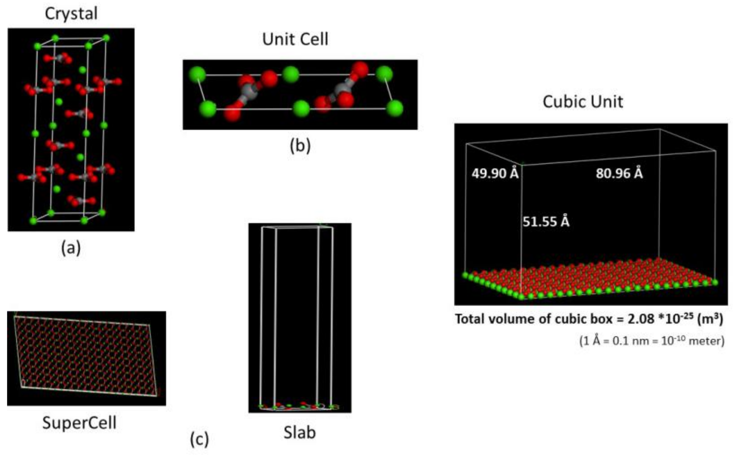
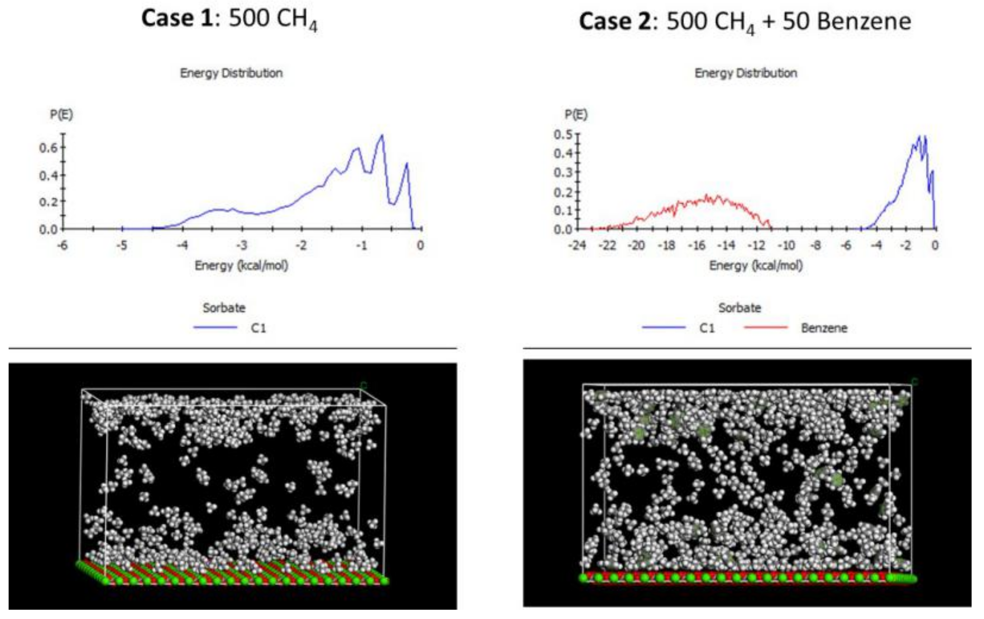
2.2. Molecular Simulation

The computational simulation of methane gas storage on the calcite surfaces of pores was conducted by Monte Carlo simulation. A unit box with dimensions of 80.96 × 49.90 × 51.55 ų was constructed with a bottom surface of calcite. The basic procedure to generate such a pore space is described as follows:

(1)

The crystal structure of calcite is taken as a = 4.99 Å, b = 4.99 Å, and c = 17.61 Å, α = 90°, β = 90°, and γ = 120° with space group R-3C (167) (Figure 1a).

(2)

The {10–14} surface of calcite is cleaved to generate a 2D unit cell (Figure 1b): a corner Ca atom is shared by four cells, so the net charge is + 0.5; a bridged Ca atom is shared by two cells, so the net charge is +1.0; the carbonate CO₃^2- species has a net charge of −2; thus, the total net charge of the unit cell is + 0.5 × 4 + 1.0 × 2 − 2 × 2 = 0.

(3)

A 10 × 10 supercell is created from the unit cell and expand to the slab high of 50 Å. Because the single calcite layer has a height of 1.55 Å, the total height of the cubic cell is 51.55 Å (Figure 1c).

Computational simulations of different methane molecules mixed with other hydrocarbon compounds adsorbed and stored within this cubic cell can thus be studied. The adsorption energies of different sorbates were calculated using canonical Monte Carlo sampling optimized with the simulated annealing method [45], where the Dreiding force field [46] was used to represent the interatomic interactions.

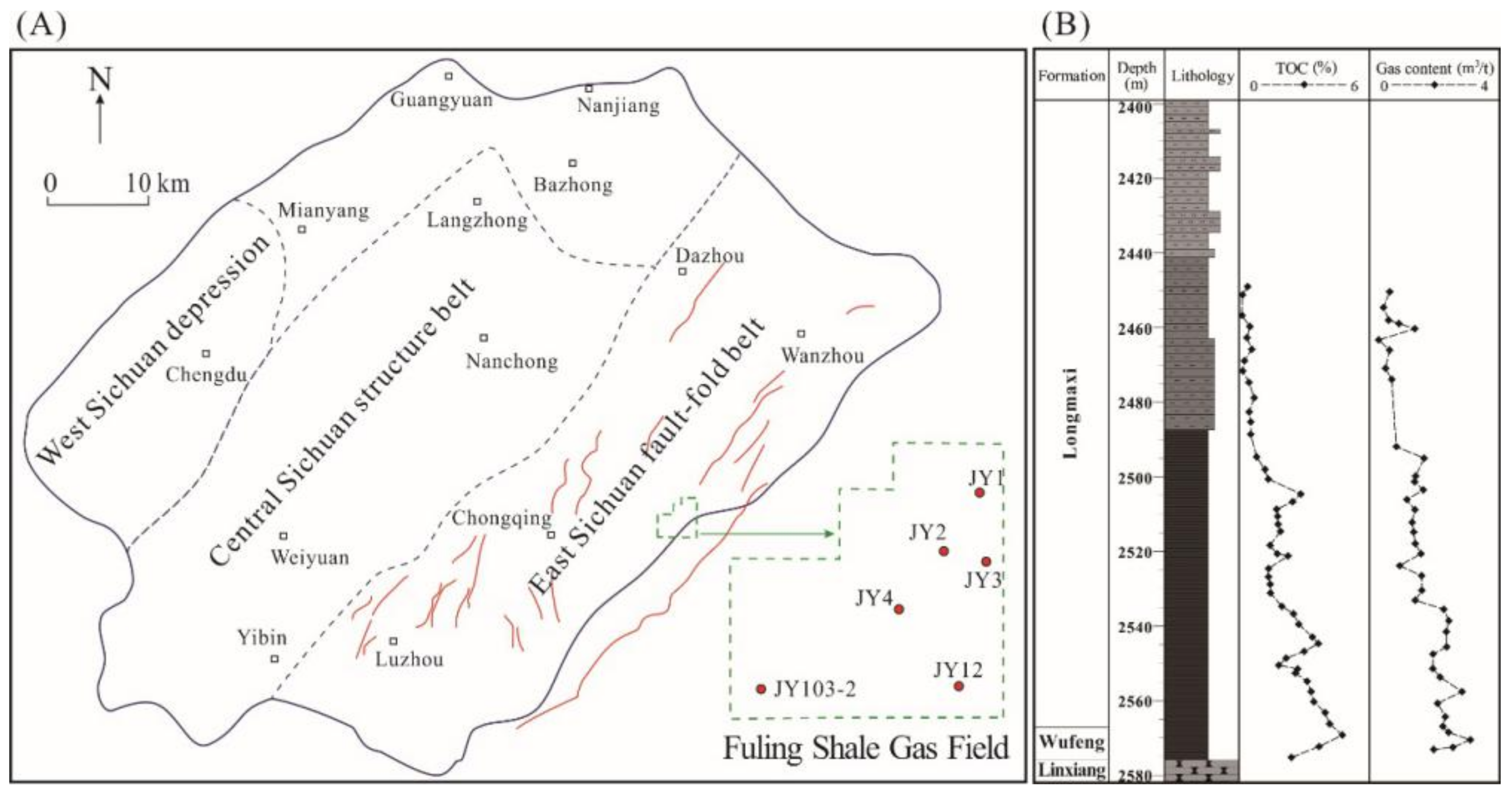
2.3. Geological Settings

The Wufeng-Longmaxi Shale succession that sedimented during the Ordovician-Silurian transition in the Sichuan Basin has been recognized as an effective source rock within and around the Sichuan Basin (Figure 2A). The Wufeng Formation is composed of organic-rich siliceous shale intercalated with a thin biolimestone, and the Longmaxi Formation is subdivided into two units. The lower unit is composed of black shale rich in organic matters (TOC > 2%), and the upper unit is dominated by gray silty mudstone interbedded with siltstone with TOC < 1% (Figure 2B).

According to the USBM method, the lower Longmaxi organic-rich shale of Well JY2 has a high gas content, ranging from 1.0 m³/t rock to 3.1 m³/t rock (Figure 2B), which supports a production capacity of 269,800 m³ per day at Well JY2. The production capacities of wells JY1, JY3, and JY4 are 203,000 m³ per day, 115,500 m³ per day, and 208,700 m³ per day, respectively. These production data suggest that the Fuling shale gas field is a favorable area for shale gas production. To date, a total shale gas volume of approximately 300 × 10⁸ m³ has been produced from the Fuling shale gas field.

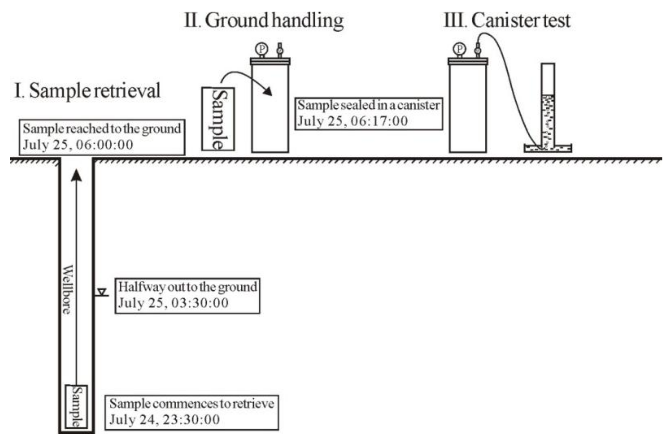
2.4. Sample and Canister Desorption

One Longmaxi Shale core sample collected from Well JY2 at a depth of 2545.65 m in the Fuling shale gas field was subjected to canister desorption at the well site (Figure 2). Figure 3 depicts the sampling procedures of this shale core from the wellbore. The key times are also noted in Figure 3. The cylindrical core sample was 0.2 m in height and 0.1 m in diameter, with a weight of 3.555 kg. The sample had a porosity of 5%, a water saturation of 30%, and a TOC content of 3 wt%. The core sample was rich in quartz (49.5%), and the clay, feldspar, carbonate, and pyrite contents were 30.4%, 5.3%, 8.9%, and 4.8%, respectively. The pore throat size distribution of a plug retrieve from the core, measured on a Micrometrics Autopore III Porosimeter in a 60,000 psi model, was divided into two size ranges at 50 nm. The content of pore throats with sizes below 50 nm was 96.8%. Methane isothermal adsorption experiments performed at 60 °C reveal that the shale sample had a Langmuir volume of 2.02 × 10⁻³ m³/kg and a Langmuir pressure of 2.855 MPa.

The canister testing followed the procedures recommended by Yee et al. [18] and Waechter et al. [17]. The core sample was quickly cleaned and weighed as soon as it was retrieved to the ground and then immediately put into a canister. The free space between the canister wall and the core sample was filled by fine sand grains to remove the air so that the accuracy of volume measurement was improved. The desorption canister was then sealed quickly and placed into a water bath that had been preheated to and maintained at approximately 53 °C.

A volume displacement apparatus was then connected to the desorption canister, and the volume of the desorbed gas was recorded automatically every 30 s. In this study, a two-stage desorption method was used to measure the total volume of desorbed gas. The first-stage desorption was conducted at 53 °C for 3 h; then, the sealed canister was heated to 110 °C with an electrical heater to rapidly collect the residual gas by enhancing the gas release rate. When the measured instantaneous gas volume fluctuated within the ±0.1% range in the last ten minutes, the measurement was terminated, and the maximum volume was recorded as the total desorbed gas volume. All the desorbed gas volumes were corrected to STP conditions [17], i.e., 0 °C and 1.01 kPa.

3. Results and Discussion

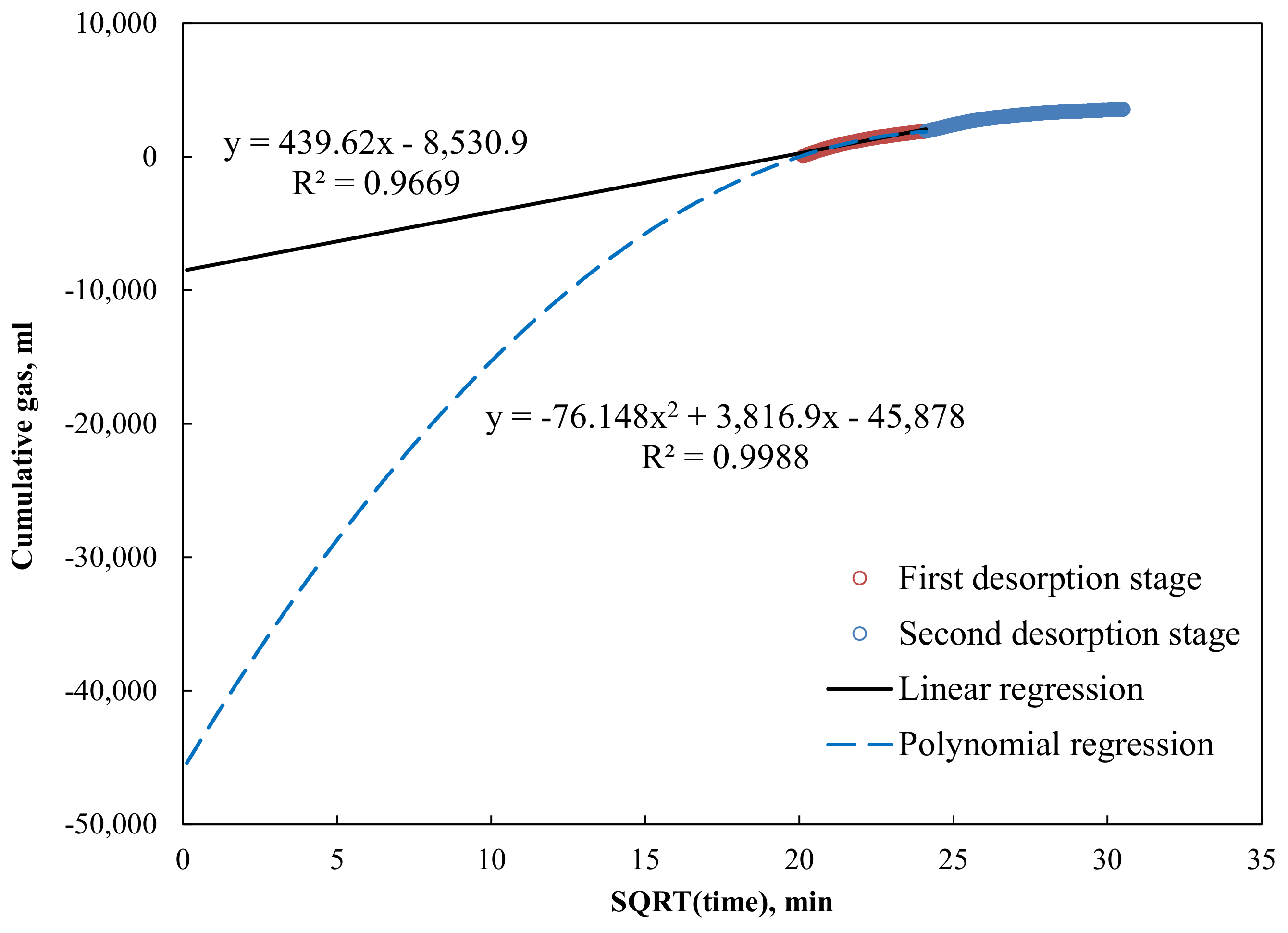
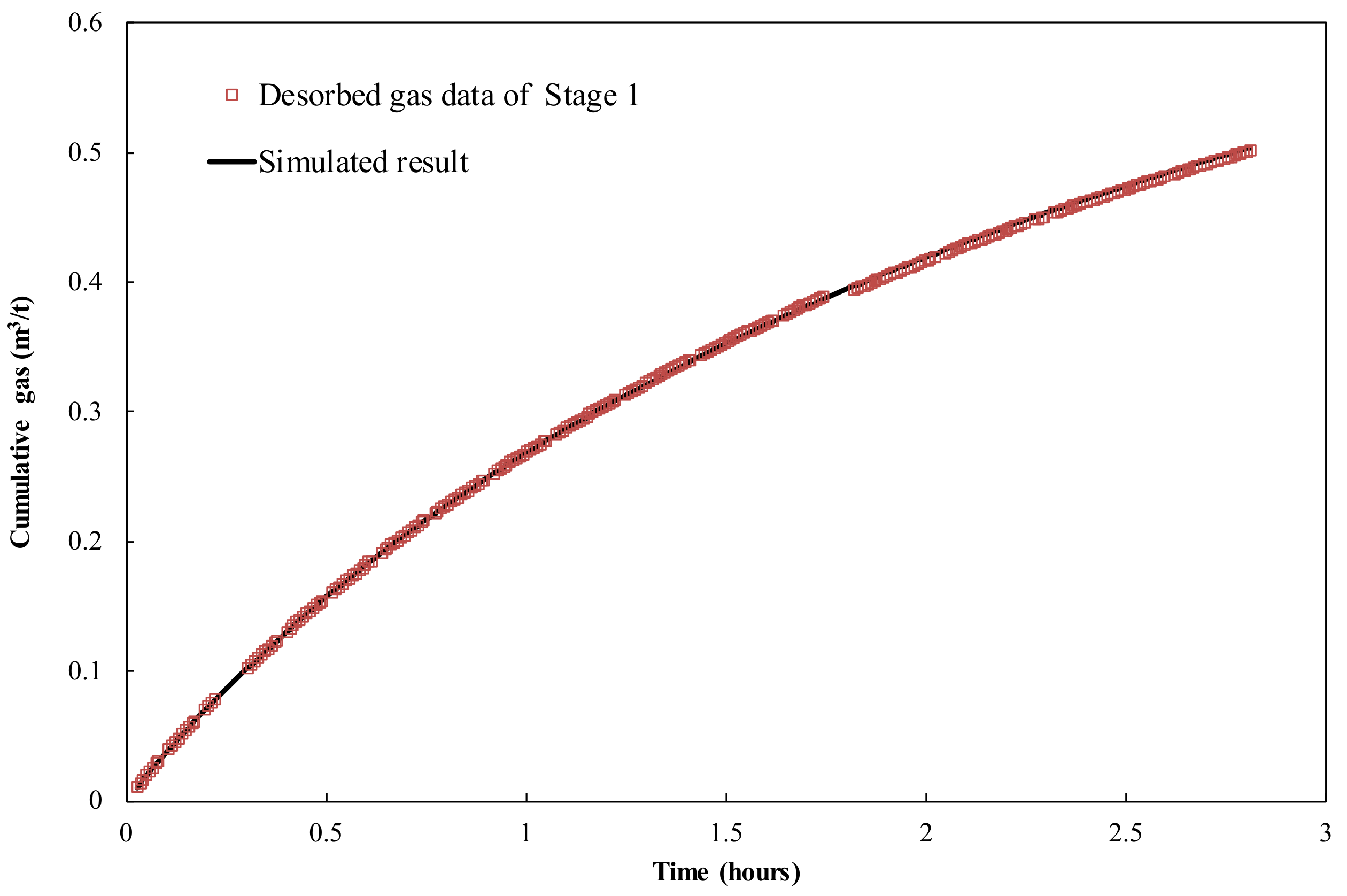
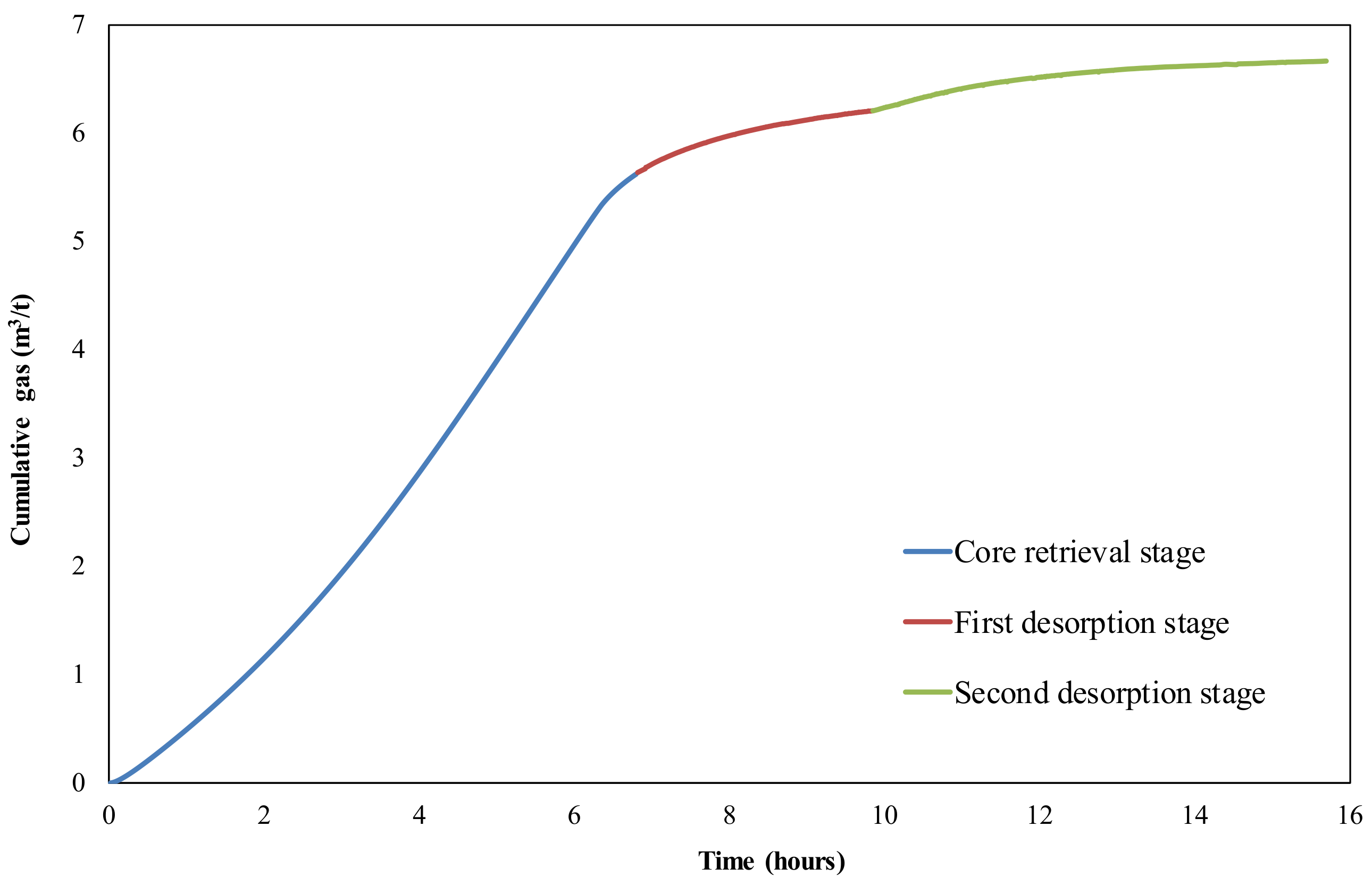
3.1. Canister Desorbed Gas and Lost Gas Calculations

Figure 4 presents the canister gas evolution with desorption time for the Longmaxi Shale core sample. It is evident that the cumulative gas volume increases gradually with desorption time, but the gas release rate gradually decreases with desorption time in the first desorption stage. Once heated to 110 °C at the beginning of the second stage, the gas release rate again increases rapidly and then decreases gradually to nearly zero. This is attributed to the reduction in methane adsorption capacity at higher temperatures [47,48].

The total volume of desorbed gas is 3.54 L (Figure 4), i.e., approximately 1.0 m³ per ton of shale. The lost gas was estimated by extrapolating the first-stage measurements to “time zero”; here, the “time zero” was determined to be when the core sample was halfway out of the boreholes [14]. The volumes of lost gas determined by means of linear regression and polynomial regression [17] are 1.11 and 3.66 m³/t rock, respectively, and thus, the total gas content derived from the polynomial regression (4.66 m³/t rock) is two times greater than that from the linear regression (2.11 m³/t rock).

Waechter et al. [17] argued that the true “time zero” should be the time when the shale core sample reaches a depth where the confining pressure equals the core pressure because considering the time at which the core is halfway out of the wellbore is only an approximation [15]. The confining pressure is related to the mud density and sample depth, and the core pressure is considered as the reservoir pressure. In the present case, the reservoir pressure of the Longmaxi Shale gas field is 37.7 MPa [49], and the density of the drilling mud used in Well JY2 was approximately 1.55 g/cm³. Therefore, the true “time zero” corresponds to a depth of 2481.9 m, which is slightly shallower than the sampling depth.

Figure 5 presents the lost gas volumes by extrapolating the desorbed gas data from the first stage to the true “time zero”. Compared with previous results (Figure 4), the lost-gas content here is 2.40 m³/t rock by linear regression, which is approximately 2.2 times the content derived from the linear extrapolation to “time zero” at a depth halfway out of the borehole, and the lost gas content by polynomial regression is 12.91 m³/t rock, which is approximately 3.5 times the content determined from the previous polynomial extrapolation to “time zero”. The total gas content derived from the polynomial regression (13.91 m³/t rock) is four times greater than that derived from the linear regression (3.40 m³/t rock).

3.2. Total Gas in Place (GIP) Based on Volumetric Approaches

There are two volumetric approaches for shale GIP calculations, the difference being whether the adsorbed-phase volume is considered [50]. The conventional volumetric approach assumes that the free gas and adsorbed gas can be determined independently of each other. On the other hand, the gas adsorbed onto the pore walls reduces the pore volume during the adsorption process, resulting in a pore volume reduction for free gas storage. Ambrose et al. [50] formulated a new GIP equation by subtracting the adsorbed phase volume from the free gas volume. That is, the effective porosity derived from helium porosimetry reflects the adsorbed gas volume and free gas volume under live reservoir conditions, for simplicity, without consideration of the water and oil volumes.

Here, the adsorbed methane density was assumed to be 370 kg/m³ [50]. The bulk methane density was assumed to be 216.32 kg/m³ based on NIST Chemistry WebBook for a pressure of 37.7 MPa and a temperature of 53 °C, the initial conditions of the Longmaxi Shale core sample. The total gas in place was calculated to be 6.56 m³/t rock with the conventional volumetric approach (Equation (12)) and 5.47 m³/t rock with the new equation (Equation (13)) proposed by Ambrose et al. [50].

$$GIP1=\frac{{\rho }_b{V}_{cylinder}{\varphi }_{cylinder}\left(1-S_w\right)}{{\rho }_{std}\cdot m_{cylinder}}+V_L\frac{P_f}{P_f+P_L}$$

(12)

$$GIP2=\frac{{\rho }_b{V}_{cylinder}{\varphi }_{cylinder}\left(1-S_w\right)}{{\rho }_{std}\cdot m_{cylinder}}+V_L\frac{P_f}{P_f+P_L}\left(1-\frac{{\rho }_b}{{\rho }_u}\right)$$

(13)

where ϕ_cylinder is the porosity of the cylinder core, V_cylinder is the volume of the cylinder core, m_cylinder is the mass of the cylinder core, S_w is the water saturation of the cylinder core, ρ_b is the bulk methane density, ρ_a is the adsorbed methane density, and P_f is the formation pressure.

3.3. Numerical Models

Here, we used the gas flow model described in Section 2.1 to fit the first stage of gas evolution data from the canister test. Figure 6 presents the fitting results of the cumulative gas volume in the first stage of gas desorption, which reflects that our model seems credible to describe the gas desorption behavior under a constant temperature. The second-order permeability model, k_a = 3.56 + 68.73/P - 5.08/P², was determined by fitting the permeability data of each time step, which is consistent with the theoretical formula [42,51]. It is evident that gas permeability decreases as pressure increases and becomes constant at 3.56 nD as pressure approaches infinity. This finding is reasonable with respect to gas dynamics because collisions between molecules are dominant in shale nanopore systems, and the slippage effect may be neglected when the pore pressure is large enough [21,34].

Lost gas volumes were calculated every 30 s as the pressure decreased from the reservoir pressure (37.7 MPa) to the average pressure of the core at the very beginning of the canister test (2.92 MPa); the confining pressure declined monotonically at a constant velocity and atmospheric pressure was maintained on the ground. The lost gas volume calculated with our model is 19.99 L (Figure 7), while the total gas volume (lost gas and desorbed gas) of this Longmaxi Shale core sample reaches 23.53 L, corresponding to a gas content of 6.62 m³/t rock. Taking into account the adsorbed phase volume, as in Ambrose’s new method, the total gas content estimated from our model is 5.88 m³/t rock.

Table 1. Total GIP results derived from different methods.

Approach	Calculation Rule	Gas Content (m3/t rock)
Direct Method	Linear extrapolation to “time zero”	2.11
	Polynomial extrapolation to “time zero”	4.66
	Linear extrapolation to true “time zero”	3.40
	Polynomial extrapolation to true “time zero”	13.91
Volumetric Approach	Conventional equation	6.56
	Ambrose’s new equation	5.47
Numerical Simulation	Ignoring adsorbed phase volume	6.62
	Considering adsorbed phase volume	5.88

lists the total GIP results derived from different methods. The GIPs using linear regression, whether extrapolating to “time zero” or true “time zero”, underestimate the gas content of Longmaxi Shale when compared with the results from volumetric approaches. The GIP using polynomial regression by extrapolating to “time zero” is also underestimated. If extrapolation to true “time zero” is performed by the polynomial fitting method, the GIP is far greater than that from the volumetric approaches. The GIPs determined using our gas flow model presented in Section 2.1 are very close to the results from the volumetric approaches, regardless of whether the adsorbed phase volume is considered.

A significant amount of lost gas was predicted with the numerical model, i.e., 19.99 L out of 23.53 L (~85%). This suggests that the majority of the shale gas is trapped within the pore space of the shale formation. The actual trapping mechanism could be associated with the microscopic structure, such as through the capillary force and overpressure effects, whereas during the sample retrieval processes, the trapped gas gains more freedom to escape.

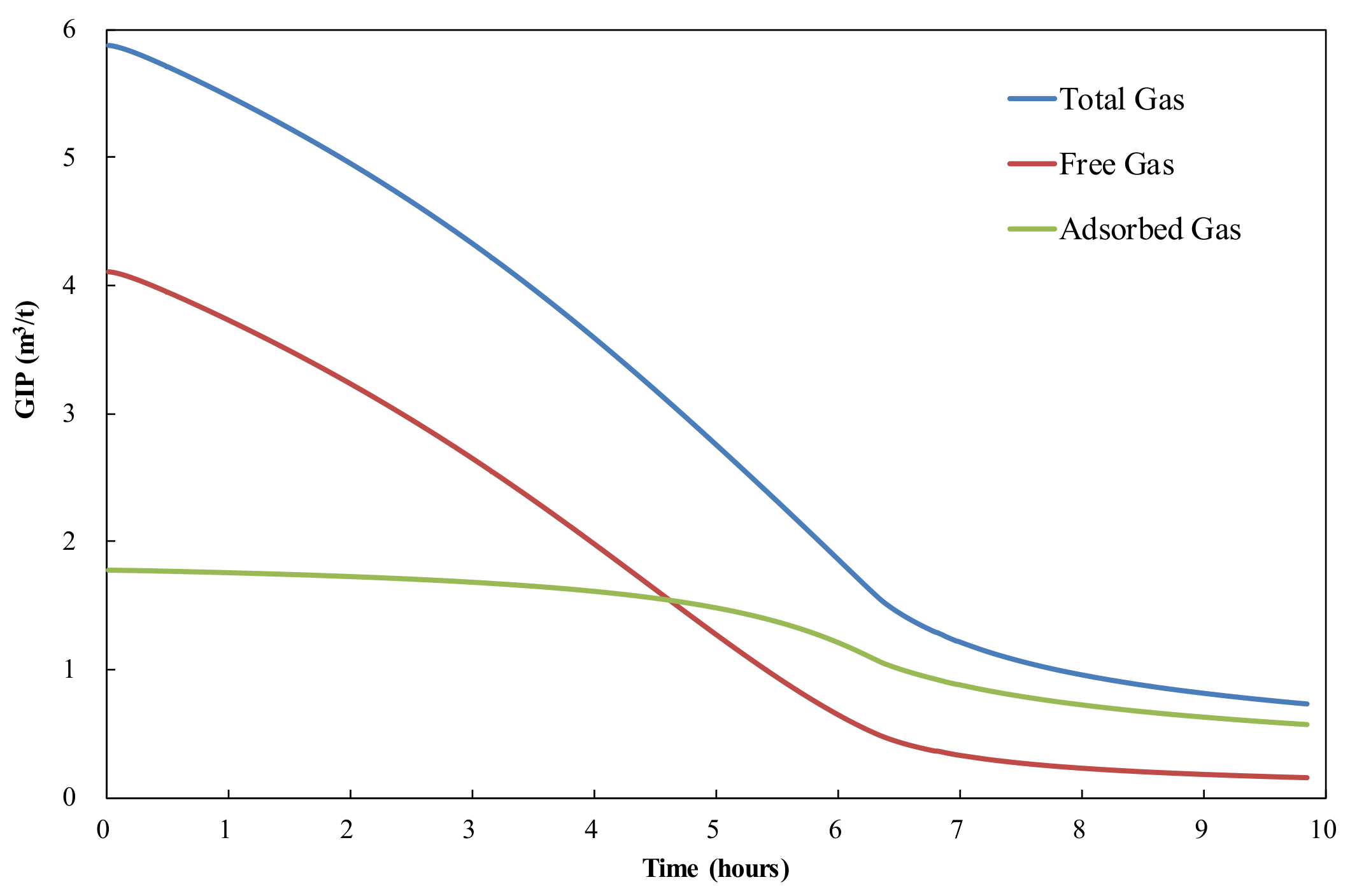
3.4. Free Gas vs. Adsorbed Gas

Based on the new equation of Ambrose et al. [50], the evolutions of total gas, free gas, and adsorbed gas calculated from the gas flow model are illustrated in Figure 8. At true “time zero”, the adsorbed gas content is 1.77 m³/t rock, accounting for 30.1% of the total gas. Usually, the adsorbed gas content in Longmaxi Shale is 20–50% [52,53]. During the first six hours, the total gas content decreases dramatically due to the expansion of free gas. Then, the total gas content decreases very slowly due to the sluggish decrease in pressure caused by gas adsorption. Approximately 4.6 h later, the content of adsorbed gas exceeds that of free gas in the core sample, and the proportion of adsorbed gas further increases with time. At the end of the first stage of gas desorption, the adsorbed gas accounts for nearly 78% of the total gas.

For the Barnett Shale, the adsorbed gas content ranges from 2.97 to 3.25 m³/t rock, accounting for 35–50% of the total gas content (4.81–7.08 m³/t rock) at a reservoir pressure of 26.2 MPa and with a formation pressure coefficient of 1.2 [54]. The adsorbed gas content of the studied Longmaxi Shale is 1.77 m³/t rock and accounts for 30.1% of the total gas content (5.88 m³/t rock) at a formation pressure of 37.7 MPa and with a formation pressure coefficient of 1.5 [49]. Methane adsorption isotherms of Longmaxi Shale with a TOC content of 3.34 wt% show that the maximum adsorbed methane capacity is less than 2.0 m³/t rock at a temperature of 50 °C [55] and that the adsorbed gas content of Longmaxi Shale reaches a plateau at approximately 10–15 MPa [56,57]. Correspondingly, the adsorbed gas content decreases by only a minor amount in the first four hours when the core pressure decreases from 37.7 to 15 MPa (Figure 7) because the available adsorption sites are fully covered by methane. The free gas content, however, increases considerably due to the increase in bulk density with compression after gas molecules take up all of the adsorptive sites. Therefore, the Longmaxi Shale has a higher free gas proportion than the Barnett Shale because the former has a larger pressure coefficient at similar depths (1.5 vs. 1.2). During degassing, a minor amount of adsorbed gas is produced until the core pressure is markedly depleted, as described by the plateau of almost saturated adsorption in the adsorption isotherm at high pressures.

In summary, the gas in the Longmaxi Shale is stored primarily as free gas, with less adsorbed gas, which is intrinsically different from the gas in CBM, which is stored mainly in the adsorbed phase. Therefore, the method of lost gas estimation based on the diffusion of CBM [13,14] leads to significant errors when it is directly applied to the evaluation of shale gas loss during the retrieval stage. Our method based on the gas flow mechanism within the shale matrix can not only calculate the GIPs objectively but also describe the evolution of free gas and adsorbed gas over time (i.e., pressure).

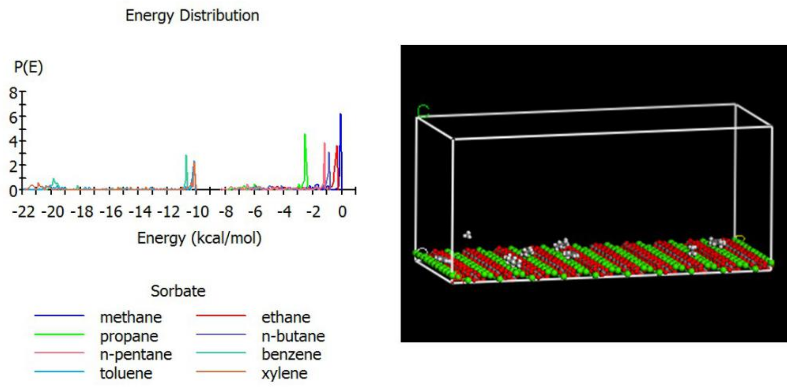
3.5. Hydrocarbon Storage in Pore Space

The calculated adsorption energies of various hydrocarbon gases—i.e., methane, ethane, propane, n-butane, n-pentane—and aromatic compounds—i.e., benzene, toluene, and xylene (often referred to as BETX)—are illustrated in Figure 9. The adsorption energies of hydrocarbon gases are mainly located in the range of −4 to 0 kcal/mol, suggesting that the chemical adsorption of hydrocarbon gases on calcite surfaces is relatively weak. Compared to that of other light hydrocarbon gases, the adsorption energy of methane is approximately zero, indicating no chemical adsorption on the calcite surface. Consequently, methane adsorption on the surface will mainly follow the Langmuir single-layer adsorption isotherm model. On the other hand, the adsorption energies of BETX aromatics are in the range of −10 kcal/mol, suggesting much stronger chemical adsorption on the calcite surface. We further calculated the adsorption of 500 methane molecules and 500 methane molecules with 50 benzene molecules on the calcite surface. The majority of the benzene (Figure 10, highlighted green) is adsorbed on the calcite surface (note: because of the periodic repetition of the unit cell, there is another calcite layer on top of the cubic cell), but the presence of BETX compounds does not significantly affect the adsorption energy of methane on the calcite surface. Therefore, methane gas is mainly stored in the pore space as the free gas rather than being adsorbed. These results indicate that the dry gas (primarily consisting of methane) is mainly confined within the pore spaces of this shale formation.

4. Conclusions

Canister tests of core samples have been widely used in the field and in laboratories to estimate the total gas in place of reservoirs. The analytical models developed for interpretation of the canister test results for conventional gas formations often fail when applied to unconventional shale reservoirs. Considering the physical process of core retrieval and the geological history and chemical compositions of shale cores, we developed and applied a mathematical model that integrates gas expansion, adsorption/desorption, and gas flow transportation in shale formations to improve shale gas assessment and prediction. The canister test results of one Longmaxi Shale core sample retrieved from Well JY2 at a depth of 2545.65 m in the Fuling shale gas field were used as field data to train and validate our theoretical model. The total gas in place values predicted with our model by taking and not taking the adsorbed phase volume into account were 5.88 and 6.65 m³/t rock, respectively. These results are more consistent with the results from the volumetric approach (5.47 and 6.56 m³/t rock, respectively), whereas the traditional analytical models for canister analysis yield larger errors (2.11 and 4.66 m³/t rock from linear and polynomial extrapolations using the traditional “time zero” approach or 3.40 and 13.91 m³/t rock from linear and polynomial extrapolations using the true “time zero” approach). In addition, our theoretical model was applied to quantitatively simulate the evolution of free gas and adsorbed gas, and the amount of lost gas (up to 85%) was determined. Molecular modeling calculations further confirm that the adsorption of methane gas on calcite surfaces is relatively weak compared to that of other hydrocarbons, suggesting that the majority of dry gas is trapped in the pore space of this shale as free gas.

References

1. United States Department of Energy. Energy Information Administration. Annual Energy Outlook 2014: With Projections to 2040; Report No.: DOE/EIA-0383(2014); United States Department of Energy: Washington, DC, USA, 2014. [Google Scholar]
2. Ross, D.J.K.; Bustin, R.M. The importance of shale composition and pore structure upon gas storage potential of shale gas reservoirs. Mar. Pet. Geol. 2009, 26, 916–927. [Google Scholar] [CrossRef]
3. Curtis, M.E. Structural characterization of gas shales on the micro-and nano-scales. In Proceedings of the Canadian Unconventional Resources and International Petroleum Conference, Calgary, AB, Canada, 19–21 October 2010. [Google Scholar] [CrossRef]
4. Slatt, R.M.; O’Brien, N.R. Pore types in the Barnett and Woodford gas shales: Contribution to understanding gas storage and migration pathways in fine-grained rocks. AAPG Bull. 2011, 95, 2017–2030. [Google Scholar] [CrossRef]
5. Chalmers, G.R.; Bustin, R.M.; Power, I.M. Characterization of gas shale pore systems by porosimetry, pycnometry, surface area, and field emission scanning electron microscopy/transmission electron microscopy image analysis: Examples from the Barnnet, Woodford, Haynesville, Marcellus, and Doig units. AAPG Bull. 2012, 96, 1099–1119. [Google Scholar] [CrossRef]
6. Clarkson, C.R.; Solano, N.; Bustin, R.M.; Bustin, A.M.M.; Chalmers, G.R.L.; He, L.; Melnichenko, Y.B.; Radlinski, A.P.; Blach, T.P. Pore structure characterization of North American shale gas reservoirs using USANS/SANS, gas adsorption, and mercury intrusion. Fuel 2013, 103, 606–616. [Google Scholar] [CrossRef]
7. Moore, T.A. Coalbed methane: A review. Int. J. Coal Geol. 2012, 101, 36–81. [Google Scholar] [CrossRef]
8. Law, B.E.; Spencer, C.W. Gas in tight reservoirs–An emerging major source of energy. In The Future of Energy Gases; U.S. Geological Survey Professional Paper 1570; United States Government Printing Office: Washington, DC, USA, 1993; p. 233. [Google Scholar] [CrossRef]
9. Curtis, J.B. Fractured shale-gas systems. AAPG Bull. 2002, 86, 1921–1938. [Google Scholar] [CrossRef]
10. Javadpour, F.; Fisher, D.; Unsworth, M. Nanoscale gas flow in shale gas sediments. J. Can. Pet. Technol. 2007, 46, 55–61. [Google Scholar] [CrossRef]
11. Etminan, S.R.; Javadpour, F.; Maini, B.B.; Chen, Z.X. Measurement of gas storage processes in shale and of the molecular diffusion coefficient in kerogen. Int. J. Coal Geol. 2014, 123, 10–19. [Google Scholar] [CrossRef]
12. Tugan, M.F.; Sinayuc, C. A new fully probabilistic methodology and a software for assessing uncertainties and managing risks in shale gas projects at any maturity stage. J. Pet. Sci. Eng. 2018, 168, 107–118. [Google Scholar] [CrossRef]
13. Bertard, C.; Bruyet, B.; Gunther, J. Determination of desorbable gas concentration of coal (Direct Method). Int. J. Rock Mech. Min. Sci. 1970, 7, 43–65. [Google Scholar] [CrossRef]
14. Kissell, F.N.; McCulloch, C.M.; Elder, C.H. The Direct Method of Determining Methane Content of Coalbeds for Ventilation Design; Report of Investigations 7767; University of Michigan Library: Ann Arbor, MI, USA, 1973; pp. 1–17. [Google Scholar]
15. McLennan, J.D.; Schafer, P.S.; Pratt, T.J. A Guide to Determining Coalbed Gas Content; Topical Report GRI-94/0396; Gas Research Institute, 1995; Available online: https://sales.gastechnology.org/Guide-to-Determing-Coalbed-Gas-Content.html (accessed on 28 September 2021).
16. Diamond, W.P.; Schatzel, S.J. Measuring the gas content of coal: A review. Int. J. Coal Geol. 1998, 35, 311–331. [Google Scholar] [CrossRef]
17. Waechter, N.B.; Hampton, G.L., III; Shipps, J.C. Overview of coal and shale gas measurement: Field and laboratory procedures. In Proceedings of the International Coalbed Methane Symposium, Tuscaloosa, AL, USA, 3–7 May 2004. [Google Scholar]
18. Yee, D.; Seidle, J.P.; Hanson, W.B. Gas sorption on coal and measurement of gas content. In Hydrocarbons from Coal; Law, B.E., Rice, D.D., Eds.; The American Association of Petroleum Geologists: Tulsa, OK, USA, 1993; pp. 203–218. [Google Scholar] [CrossRef]
19. Diamond, W.P.; Schatzel, S.J.; Garcia, F.; Ulery, J.P. The Modified Direct Method: A Solution for Obtaining Accurate Coal Desorption Measurements; International Coalbed Methane Symposium: Tuscaloosa, AL, USA, 2001; pp. 331–342. [Google Scholar]
20. Shtepani, E.; Noll, L.A.; Elrod, L.W.; Jacobs, P.M. A new regression-based method for accurate measurement of coal and shale gas content. SPE Reserv. Eval. Eng. 2012, 13, 359–364. [Google Scholar] [CrossRef]
21. Javadpour, F. Nanopores and gas permeability of gas flow in mudrocks (Shales and Siltstone). J. Can. Pet. Technol. 2009, 48, 16–21. [Google Scholar] [CrossRef]
22. Shabro, V.; Torres-Verdín, C.; Javadpour, F. Numerical simulation of shale-gas production: From pore-scale modeling of slip-flow, Knudsen diffusion, and Langmuir desorption to reservoir modeling of compressible fluid. In Proceedings of the SPE North American Unconventional Gas Conference and Exhibition, The Woodlands, TX, USA, 14 June 2011. [Google Scholar] [CrossRef] [Green Version]
23. Shabro, V.; Torres-Verdín, C.; Sepehrnoori, K. Forecasting gas production in organic shale with the combined numerical simulation of gas diffusion in kerogen, Langmuir desorption from kerogen surfaces, and advection in nanopores. In Proceedings of the SPE Annual Technical Conference and Exhibition, San Antonio, TX, USA, 8–10 October 2012. [Google Scholar] [CrossRef]
24. Hosseini, S.A.; Javadpour, F.; Michael, G.E. Novel analytical core-sample analysis indicates higher gas content in shale-gas reservoirs. SPE J. 2015, 20, 1–12. [Google Scholar] [CrossRef]
25. Metwally, Y.M.; Sondergeld, C.H. Measuring low permeabilities of gas-sands and shales using a pressure transmission technique. Int. J. Rock Mech. Min. Sci. 2011, 48, 1135–1144. [Google Scholar] [CrossRef]
26. Ghanizadeh, A.; Gasparik, M.; Amann-Hildenbrand, A.; Gensterblum, Y.; Krooss, B.M. Experimental study of fluid transport processes in the matrix system of the European organic-rich shales: I. Scandinavian Alum Shale. Mar. Pet. Geol. 2014, 51, 79–99. [Google Scholar] [CrossRef]
27. Bhandari, A.R.; Flemings, P.B.; Polito, P.J.; Cronin, M.B.; Bryant, S.L. Anisotropy and stress dependence of permeability in the Barnett Shale. Transp. Porous Media 2015, 108, 393–411. [Google Scholar] [CrossRef]
28. Ma, Y.; Pan, Z.; Zhong, N.; Connell, L.D.; Down, D.I.; Lin, W.; Zhang, Y. Experimental study of anisotropic gas permeability and its relationship with fracture structure of Longmaxi Shales, Sichuan Basin, China. Fuel 2016, 180, 106–115. [Google Scholar] [CrossRef]
29. Kunda, P.K.; Cohen, I.M.; Dowling, D.R. Fluid Mechanics, 5th ed.; Elsevier Academic Press: Cambridge, MA, USA, 2012; pp. 96–99. [Google Scholar]
30. Cui, X.; Bustin, A.M.M.; Bustin, R.M. Measurements of gas permeability and diffusivity of tight reservoir rocks: Different approaches and their applications. Geofluids 2009, 9, 208–223. [Google Scholar] [CrossRef]
31. Mattar, L.; Brar, G.S.; Aziz, K. Compressibility of natural gases. J. Can. Pet. Technol. 1975, 14, 77–80. [Google Scholar] [CrossRef]
32. Ghedan, S.G.; Aljawad, M.S.; Poettmann, F.H. Compressibility of natural gases. J. Pet. Sci. Eng. 1993, 10, 157–162. [Google Scholar] [CrossRef]
33. Lohrenz, J.; Bray, B.G.; Clark, C.R. Calculating viscosities of reservoir fluids from their compositions. J. Pet. Technol. 1964, 16, 1171–1176. [Google Scholar] [CrossRef]
34. Freeman, C.M.; Moridis, G.J.; Blasingame, T.A. A numerical study of microscale flow behavior in tight gas and shale gas reservoir systems. Transp. Porous Media 2009, 90, 253–268. [Google Scholar] [CrossRef]
35. Darabi, H.; Ettehad, A.; Javadpour, F.; Sepehrnoori, K. Gas flow in ultra-tight shale strata. J. Fluid Mech. 2012, 710, 641–658. [Google Scholar] [CrossRef]
36. Firouzi, M.; Alnoaimi, K.; Kovscek, A.; Wilcox, J. Klinkenberg effect on predicting and measuring helium permeability in gas shales. Int. J. Coal Geol. 2014, 123, 62–68. [Google Scholar] [CrossRef]
37. Kazemi, M.; Takbiri-Borujeni, A. An analytical model for shale gas permeability. Int. J. Coal Geol. 2015, 146, 188–197. [Google Scholar] [CrossRef]
38. Tang, G.H.; Tao, W.Q.; He, Y.L. Gas slippage effect on microscale porous flow using the lattice Boltzmann method. Phys. Rev. E 2005, 72, 056301. [Google Scholar] [CrossRef] [PubMed]
39. Moghadam, A.A.; Chalaturnyk, R. Expansion of the Klinkenberg’s slippage equation to low permeability porous media. Int. J. Coal Geol. 2014, 123, 2–9. [Google Scholar] [CrossRef]
40. Moghaddam, R.N.; Jamiolahmady, M. Slip flow in porous media. Fuel 2016, 173, 298–310. [Google Scholar] [CrossRef]
41. Yang, Y.; Bao, F. Characteristics of shale nanopore system and its internal gas flow: A case study of the lower Silurian Longmaxi Formation shale from Sichuan Basin, China. J. Nat. Gas Geosci. 2017, 2, 303–311. [Google Scholar] [CrossRef]
42. Maurer, J.; Tabeling, P.; Joseph, P.; Willaime, H. Second-order slip laws in microchannels for helium and nitrogen. Phys. Fluids 2003, 15, 2613–2621. [Google Scholar] [CrossRef]
43. Sakhaee-Pour, A.; Bryant, S.L. Gas permeability of shale. SPE Reserv. Eval. Eng. 2012, 15, 401–409. [Google Scholar] [CrossRef]
44. Dongari, N.; Agrawal, A.; Agrawal, A. Analytical solution of gaseous slip flow in long microchannels. Int. J. Heat Mass Transf. 2007, 50, 3411–3421. [Google Scholar] [CrossRef]
45. Kirkpatrick, S.; Gelatt, C.D.; Vecchi, M.P. Optimization by Simulated Annealing. Science 1983, 220, 671–680. [Google Scholar] [CrossRef]
46. Mayo, S.L.; Olafson, B.D.; Goddard, W.A. DREIDING: A generic force field for molecular simulation. J. Phys. Chem. 1990, 94, 8897–8909. [Google Scholar] [CrossRef]
47. Rexer, T.F.T.; Benham, M.J.; Aplin, A.C.; Thomas, K.M. Methane adsorption on shale under simulated geological temperature and pressure conditions. Energy Fuels 2013, 27, 3099–3109. [Google Scholar] [CrossRef] [Green Version]
48. Li, T.; Tian, H.; Xiao, X.; Cheng, P.; Zhou, Q.; Wei, Q. Geochemical characterization and methane adsorption capacity of overmature organic-rich Lower Cambrian shales in northeast Guizhou region, southwest China. Mar. Pet. Geol. 2017, 86, 858–873. [Google Scholar] [CrossRef]
49. Guo, T. The Fuling Shale Gas Field—a highly productive Silurian gas shale with high thermal maturity and complex evolution history, southeastern Sichuan Basin, China. Interpretation 2015, 3, SJ25–SJ34. [Google Scholar] [CrossRef]
50. Ambrose, R.J.; Hartman, R.C.; Diaz-Campos, M.; Akkutlu, I.Y.; Sondergeld, C.H. Shale gas-in-place calculations Part I: New pore-scale considerations. SPE J. 2012, 17, 219–229. [Google Scholar] [CrossRef]
51. Beskok, A.; Karniadakis, G.E. Report: A model for flows in channels, pipes, and ducts at micro and nano scales. Microscale Thermophys. Eng. 1999, 3, 43–77. [Google Scholar] [CrossRef]
52. Gou, Q.; Xu, S. Quantitative evaluation of free gas and adsorbed gas content of Wufeng-Longmaxi shales in the Jiaoshiba area, Sichuan Basin, China. Adv. Geo-Energy Res. 2019, 3, 258–267. [Google Scholar] [CrossRef] [Green Version]
53. Pang, X.; Chen, G.; Xu, C.; Tong, M.; Ni, B.; Bao, H. Quantitative evaluation of adsorbed and free gas and their mutual conversion in Wufeng-Longmaxi shale, Fuling area. Oil Gas Geol. 2019, 40, 1248–1258. (In Chinese) [Google Scholar]
54. Montgomery, S.L.; Jarvie, D.M.; Bowker, K.A.; Pollastro, R.M. Mississippian Barnett Shale, Fort Worth basin, north-central Texas: Gas-shale play with multi-trillion cubic foot potential. AAPG Bull. 2005, 89, 155–175. [Google Scholar] [CrossRef]
55. Tian, H.; Li, T.; Zhang, T.; Xiao, X. Characterization of methane adsorption on overmature Lower Silurian-Upper Ordovician shales in Sichuan Basin, southwest China: Experimental results and geological implications. Int. J. Coal Geol. 2016, 156, 36–49. [Google Scholar] [CrossRef]
56. Yang, F.; Ning, Z.; Zhang, R.; Zhao, H.; Krooss, B.M. Investigation on the methane sorption capacity of marine shales from Sichuan Basin, China. Int. J. Coal Geol. 2015, 146, 104–117. [Google Scholar] [CrossRef]
57. Pan, L.; Xiao, X.; Tian, H.; Zhou, Q.; Cheng, P. Geological models of gas in place of the Longmaxi shale in Southeast Chongqing, South China. Mar. Pet. Geol. 2016, 73, 433–444. [Google Scholar] [CrossRef]
Figure 1. Construction of a calcite-based cubic cell. (a) The crystal structure of calcite. (b) The {10-14} surface of calcite is cleaved to generate a 2D unit cell. (c) A 10 × 10 supercell is created from the unit cell and expand to the slab high of 50 Å.
Energies 14 06518 g001
Figure 2. (A) Location of the Fuling shale gas field in the Sichuan Basin. (B) Lithological profile of Well JY2 in the Fuling shale gas field. The gas content data were calculated according to the USBM “Direct Method”.
Energies 14 06518 g002
Figure 3. Shale core sampling procedure for canister testing in the field (the real times related to the canister test used in this study are noted in rectangles).
Energies 14 06518 g003
Figure 4. The results of a canister test of a shale core sample from the Longmaxi Formation from Fuling shale gas field in the Sichuan Basin. Desorption is divided into two stages: the first stage is at 53 °C and lasts for 3 h, and the second stage is at 110 °C and lasts until the end of the test. The volume of lost gas is determined by extrapolating the first-stage measurements to “time zero” by linear or polynomial regression. The volumes of lost gas are 3.95 L and 13.02 L, respectively.
Energies 14 06518 g004
Figure 5. Extrapolation of canister desorbed gas data extrapolated to the true “time zero” to determine the lost gas volumes of 8.53 L and 45.88 L by linear regression and polynomial regression, respectively.
Energies 14 06518 g005
Figure 6. Results of the first-stage cumulative gas volume modeling using Equation (11).
Energies 14 06518 g006
Figure 7. The evolution of cumulative gas volume of the observed shale core sample.
Energies 14 06518 g007
Figure 8. The evolution of total gas, free gas, and adsorbed gas from “time zero” to the end of first stage of desorption from our model.
Energies 14 06518 g008
Figure 9. Calculated adsorption energies (kcal/mol) on a calcite surface in a pore space.
Energies 14 06518 g009
Figure 10. Calculated adsorption energies (kcal/mol) on a calcite surface in a pore space.
Energies 14 06518 g010