Abstract
Gas flaring represents a large waste of a natural resource for energy production and is a significant source of greenhouses gases to the atmosphere. The World Bank estimates annual flared gas volumes of 150 billion cubic meters, based upon a conversion of remotely sensed radiant heat data from the NOAA’s VIIRS (Visible Infrared Imaging Radiometer Suite) instrument onboard the polar-orbiting Suomi NPP satellite. However, the conversion of the remotely sensed radiant heat measurements into flared gas volumes currently depends on flare operator reported volumes, which can be biased in various ways due to inconsistent reporting requirements. Here, I discuss both known and unknown biases in the datasets, using them to illustrate the current lack of accuracy in the widely discussed flaring numbers. While volume trends over time could be derived directly from the radiant heat data, absolute amounts remain questionable. Standardizing how flared gas volumes are measured and reported could dramatically improve accuracy. In addition, I suggest expanding satellite measurements of individual flares burning under controlled conditions as a major improvement to daily monitoring, alongside the potential usage of remotely sensed flare temperature to estimate combustion efficiency.
1. Introduction
As the international discussion about how best to address climate change this decade is rapidly advancing, single, large man-made sources of greenhouse gas (GHG) emissions stand out. Of particular interest in the last decade has been atmospheric methane. Increasing again since the mid 2000s [1], geoscientists have scrutinized its sources and recently concluded that a combination of two dominant anthropogenic sources are to blame: the increased mining, distribution, and use of fossil gas, and the rise of biogenic methane emissions, largely related to enteric fermentation and animal wastes [2]. Both of these large emission sources are under man-made control, meaning their abatement is possible and desirable in the context of GHG emission reduction plans. Both past evaluations and a more recent work [3,4,5] have shown that the associated methane emission reductions would be effective in reducing both the rate of global warming as well as the ultimate level of warming by 2100, in various scenarios of development.
Methane emissions from the fossil fuel sector are dominated by (fugitive) emissions from upstream oil and gas production as well as coal bed/seam venting during mining [6]. Among the former, emissions are caused by numerous practices in the oil and gas industry that could be abated or avoided, such as gas venting and flaring [7]. While venting occurs regularly for both maintenance and operational purposes, gas flaring is most common at oil production sites, where the flare disposes of the gas associated with the more valuable product, oil. Associated gas flaring at upstream facilities dominates worldwide flaring volumes [8]. It is estimated to represent nearly 1% of anthropogenic CO2 emissions [9]. However, the combustion efficiency of gas flares at upstream oil production sites is poorly characterized, and even if the standard assumption of 98% combustion efficiency such as implemented for the US-EPA’s GHG reporting program (CFR 40, §98.233(n)) were correct—anecdotal evidence suggests that for many flares it is likely to be substantially lower—gas flares would still present a significant source of methane to the atmosphere [10,11].
Gas flares, whether upstream or downstream, are generally operated with an open flame. To-be disposed of hydrocarbons are piped toward a flare stack (ground flares are uncommon), and condensable components may be reduced in a “knock-out drum” before the gas enters the stack [12]. Flare stack dimensions and height are determined by the waste gas volumes that require disposal, and the required distance from heat radiation from combustion, respectively. A pilot light is typically needed to assure ignition, and a specially designed flare tip may be used to facilitate fuel-air mixing [12]. While steam- or air-assisted flares are common in downstream industrial applications, where they are used to optimize combustion efficiency [13,14,15], they are rare in upstream flare operations, which dominate global gas flaring volumes. The latter, called diffusion flares, may have widely varying combustion efficiencies and associated methane and air pollutant emission characteristics [11,16,17].
Gas flaring in the global oil industry in general is poorly quantified. Flaring occurs for safety reasons if the associated gas cannot be used or stored, such as at offshore platforms. When the gas could be but is not used due to a lack of financial or other incentives, the practice is called “routine flaring”. The majority of such flares is highly visible, especially at night. They represent an enormous waste of a natural resource [8,11,18,19,20], while, at the same time, acting as a local source of air pollution due to incomplete combustion and the generation of NOx [21,22,23]. Routine flaring, therefore, has become a target of environmental groups, which demand its reduction and eventual elimination [24].
To address routine flaring as a source of GHG emissions and local air pollution, however, reliable data on flaring volumes and changes over time are required. In this context, the development of a satellite based dataset of flare locations, flare temperatures, and estimated flaring volumes, and its use by the World Bank [18] and other entities have become important tools to monitor flaring activities, and to provide stakeholders with up-to-date information on a wasted resource and its emissions. Here, I briefly revisit how the satellite data are utilized to estimate flaring volumes, how those volumes could be biased in various ways, and what is necessary to improve these estimates going forward.
2. Estimating Flaring Volumes from Satellite Data
Since there have recently been two new web-portals (http://flaringmonitor.com; http://flareintel.com, both accessed on 4 October 2021) initiated that are using the satellite data to provide “on demand” flaring volume estimates to commercial and non-commercial customers, it is useful to revisit how those gas volumes are calculated and what we can currently say about their accuracy.
Both web-portals use provided daily infrared radiance data from the VIIRS instrument, managed by the Earth Observation Group (EOG) at the Colorado School of Mines [25]. The radiance data are filtered to focus on sources most likely originating in gas flares vs. other heat sources, such as e.g., industrial heat sources and wildfires [25,26]. The next step is critical, as it involves the conversion of this heat radiation into flared gas volumes. The required information for this conversion currently comes from government data, often publicly available, and originates from operator reported “gas disposition”.
Oil and gas producers worldwide collect and report “disposition” data for their products, in this case oil and gas amounts, typically monthly or annually, which includes amounts sent to market and otherwise. In the US, for example, companies report these amounts to state regulatory agencies. Gas that was produced but not used locally or sent to market (e.g., via pipeline) has historically been reported as “vented or flared”. Not all jurisdictions require reporting that distinguishes between these two dispositions. Notably, any gas amount vented is undetectable by the VIIRS instrument, which relies on the detection of heat produced during its combustion. Assuming the reported flaring volumes are correct, a correlation of the satellite measured radiant heat (RH) against the volume data serves to calibrate the nightly measured RH data and convert them to flaring volumes.
The original work by Elvidge et al. [25] used a database housed by Cedigaz, an international, country-specific venting and flaring volume database containing 2012–2014 data (not publicly available). The EOG group combined reported annual total volumes with accumulated annual RH data for each reporting country for a macro-scale calibration, which can be accessed and viewed online (https://eogdata.mines.edu/download_global_flare.html, accessed on 4 October 2021). A very similar methodology is used by one of the new web-portals. As explained in its white paper [27], independent calibrations between reported venting and flaring and accumulated RH data were developed for different (oil) production regions, down to individual operators in those regions, by clustering the radiance data. This creates slightly different slopes of the calibration line, now a meso-scale calibration, but not necessarily a more accurate calibration. While the original calibration by the EOG group [25] considered the reported volumes to be the independent variable (x-values), BAZEAN considered the clustered RH data as the independent variable in their linear regression. In both cases, though, it appears that an ordinary least squares (OLS) regression was used to determine the slope (conversion factor), a statistical procedure that assumes no error in the x-axis data, and thus produces an underestimate of the slope.
Using either macro- or meso-scale calibrations allows downscaling, all the way down to an individual flare, the heat signature of which can be observed each night during 1–2 short overpass period(s) depending on geographic location (Figure 1a). The conversion factors from the regional calibrations, or the global macro-calibration, thus allow direct estimation of flaring volumes on a daily basis.
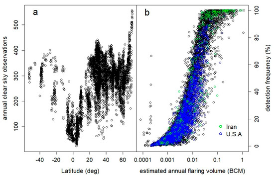
Figure 1.
(a) Available clear-sky flare observations by VIIRS in 2019 versus latitude; (b) 2019 detection frequency (ratio of observations of a flare detected under cloud-free conditions to total observations for that location under cloud-free conditions) as a function of estimated flaring volume (BCM = billion cubic meters, per year), demonstrating that large flares operate nearly continuously, while small flares tend to be intermittent.
3. Known and Unknown Biases
The calibration procedure described above disregards several known and unknown biases in both datasets, which can cause the flaring volume estimates to be highly uncertain. They do not make the derived estimates useless, but they should require a distinction between absolute amounts and relative changes over time.
The obvious, known biases include
- reported volumes containing a significant fraction of gas that was not combusted upon wasting it, aka venting. The original calibration assumed the reported volumes as the independent variable (knowns), so if the actually combusted volumes are smaller (e.g., by a factor of 0.9, aka 90% flaring, 10% venting), but the calibration assumes that 100% of reported volumes are flared (the default), and a given cumulative RH observation in turn translates into a larger volume than was actually combusted. In that case, flaring would be overestimated by 10%. In the publically available information, reported volumes are often not distinguished between vented and flared; instead, a sum is reported. In addition, there is no available information that would allow us to correct for this bias.
- different rules among different agencies and countries with respect to what gas disposition is actually in need of reporting. There are numerous exemptions upstream operators are given during periods of drilling, completions, and maintenance. Venting or flaring volumes during these periods may either not be known, estimated or metered, or may simply not be reported. The associated rules are not uniform, not even nationally. This bias exists by design of deeming certain volumes unimportant, and it leads to a default underestimation of venting and flaring in the reporting database, but not one that could be corrected for because of a lack of input data.
- the satellite recording radiant heat emissions generally only once daily during a nighttime overpass. The representativeness of such a measurement depends on a flare operating near continuously under a steady gas stream. However, many flares worldwide do not burn steadily all the time. Intermittency and at times violent fluctuations, depending on gas flow rates, liquid hydrocarbon entrainment, or ambient wind conditions, are not uncommon. In addition, as soon as a flare is reduced to a small flame (low volume combustion), the satellite sensor cannot track it any longer due to low signal-to-noise ratios. In shale oil production fields such as in the US, thousands of small volume flares at low production sites were not detected [28]. They may not add much to the total volume flared in a region, yet present a bias nevertheless.
- weather conditions affecting RH detection. Because the satellite instrument cannot “see” through clouds, the detection frequency of flares in different parts of the world may fluctuate with cloudiness. Part of the non-perfect macro-scale calibration [25] may stem from cloud cover variability (Figure 1a). For a particular region of the globe, this does not likely manifest as a bias over the long-run (annual data), but could on shorter time scales given that, depending on the local climatology, cloudiness can change on a seasonal basis, and the fractional adjustments currently made may properly correct the volumes only for frequently detected flares. Accumulated radiances for the same amount of gas flared can be different between regions of vastly different cloudiness, and regional meso-scale calibrations are thus a better choice than the macro-scale calibration.
In addition, there is likely an unknown bias in the reporting databases that has to do with a lack of actual measurements and of auditing the numbers. Oil and gas producers do not uniformly use approved gas metering devices in or on pipes feeding flares [29]. Thus, many, possibly most reported volumes, are based on engineering calculations, which may not have been tested against direct measurements in the field. Even hand-waving may occur when input data are lacking. Furthermore, upstream gas flares are not monitored in the field for effective operation. So why do we think we can trust the reported volumes?
Since bottom-up, reported flaring volumes enter the satellite data calibration, accurate volumes in the reporting databases are crucial. Based purely upon physics, the correlation between instantaneous or accumulated volumes combusted and the associated RH emissions observed by the satellite sensor should be very tight, and that is exactly what the EOG group found in a pilot study on 24 flares operated under different flow rates at a test facility in Tulsa, Oklahoma [30]. Therefore, the large inconsistencies in the macro-scale calibration [25] are probably due to inconsistencies in the reporting database.
4. Possible Improvements Going Forward
A more accurate accounting of flaring worldwide has to consider the above known biases in both datasets and the unknown biases in the reporting database. The current, and questionable, assumption is that we can trust the monthly and/or annually reported volumes, and then use the satellite data to derive fluctuations. Given the circumstances, this is ok as long as there is an understanding that the derived volumes are not accurate, and could be biased in either direction on various spatial and temporal scales. However, unless the calibration changes over time (e.g., due to trends in cloudiness), comparisons on a relative basis derived from the satellite data, such as annual trends, are expected to be precise, at least on a regional basis, even though absolute values may be biased.
A recent case study by Brandt [31] illustrates the general “accuracy” of satellite based flaring volume estimates when several of the above listed biases are likely minimal. Brandt analyzed offshore flares of seven countries with governmental record-keeping, with a focus on easily detectable, generally large flares on platforms and floating production units [31]. In these cases, possible biases in the satellite data stemming from cloudiness, detectability or detection frequency are minimized. The included flares belong to a subset of flares that combust gas steadily, generally at above average volumes and, even if not metered, likely under known composition and production conditions that make engineering estimates of the combusted volume accurate. The resulting volume comparison showed order of magnitude, yet comparatively modest biases in both directions, which canceled each other on aggregate scales. This result is different from earlier work showing large biases for land-based flares in Texas [28], most of which operate intermittently (Figure 1b), illustrating the wide range of results that can be expected in such studies based upon two very different input databases.
To increase the accuracy of such comparisons, and especially of flaring emissions created by the intermittent and smaller flares that dominate the flare numbers (Figure 1b) [25], reporting has to be improved for at least two items: (i) venting needs to be reported independent of flaring, nationally and internationally; this would produce an important co-benefit in that it would improve our knowledge about venting-associated methane emissions, recently highlighted by Zhang and coworkers [32]; (ii) both venting and flaring emissions need to be based upon actual measurements (metering flows) whenever possible and ought to be reported above lower thresholds than is currently the case.
In addition, micro-scale calibrations should be utilized. This can be accomplished by determining radiant heat emissions from controlled flares with measured gas compositions, accurately metered flow, flare temperature, and measured combustion efficiency [13], ideally at several field sites and for a range of gas compositions and flare sizes, expanding upon the pilot study by Zhizhin et al. [30] (I note that the flare volume estimates in the commercial flareintel pro version are already based upon such micro-calibrations the company developed with collaboration from operators).
When a flare is large enough, the satellite data based determination of flare temperature is an additional, potentially very useful data point, one possibly related to combustion efficiency. Figure 2 shows flare temperature, when available, as a function of detection frequency for the 2019 global data set provided by the EOG group. Because detection frequency is strongly related to estimated flaring volume (Figure 1b), the result is a weak but significant correlation between flaring volume and flare temperature (not shown). Large flares operating most of the time, and resulting in large annual flaring volumes (Figure 1b), such as approximately 20% of all flares in Iran that roughly follow the 80/20 rule, tend on average to be 175 K cooler than typical U.S. flares in shale oil production areas detected only 10% of the time (median values, 1710 vs. 1885 K, Figure 2). Since adiabatic flame temperatures do not change very much with the gas’ lower hydrocarbon composition, it stands to reason that incomplete combustion may be related to lower flame temperatures [23,33]. This is consistent with larger gas volumes requiring air or steam assisted flares to achieve an optimal combustion efficiency, but such assistance rarely practiced at upstream oil production sites. Furthermore, a recent study by Kumar and coworkers [34] suggests that the soot from smoking flares can affect the radiative power received at the satellite IR heat sensor. A smoking flare burns its hydrocarbons inefficiently [13], and this may lead to a useful relationship between remotely sensed flare temperature and combustion efficiency.
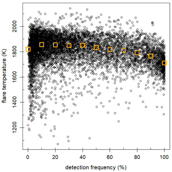
Figure 2.
Average flare temperatures as a function of detection frequency (2019 data), illustrating that high detection frequencies, associated with the largest estimated flaring volumes (Figure 1b), are related to flares with lower remotely sensed flame temperatures. Orange squares mark 10%-binned (0–5%, 5–15%, 15–25%, etc.), median flare temperatures per detection frequency bin.
If the VIIRS flare data flame temperatures can be exploited this way, a question answerable via a micro-scale calibration, it would allow the estimation of methane slip as an additional, highly valuable data point. Furthermore, if companies operating flares metered volume flow rates electronically as has been recommended over a decade ago [29], they could also report the variability of these flow rates to their flares, which would provide an estimate of the range of daily volume flow rates as determined from a single nighttime measurement at the hour of the satellite instrument’s flyover. That way, volume estimates from the satellite RH data conversions would become more constrained on shorter than monthly time scales.
5. Conclusions
Current estimates of worldwide gas flaring volumes are uncertain, possibly underestimated due to various biases in both the satellite data and the reporting databases used to calibrate the conversion factors. Recent improvements to the original macro-scale calibration use regional meso-scale calibrations, but still suffer from biased reporting databases. Only well-planned micro-scale calibrations can achieve a major step forward in quantification accuracy, which is needed to make optimum usage of the satellite measurement capabilities.
Funding
The author received no funding for this work.
Institutional Review Board Statement
Not applicable.
Informed Consent Statement
Not applicable.
Data Availability Statement
The data used in this manuscript is publically available at https://eogdata.mines.edu/download_global_flare.html (accessed on 4 October 2021).
Acknowledgments
The author thanks David Lyon at EDF, and Mark Davis from Capterio for feedback. The open access publishing fees for this article have been covered by the Texas A&M University Open Access to Knowledge Fund (OAKFund), supported by the University Libraries.
Conflicts of Interest
The author declares no conflict of interest.
References
- Turner, A.J.; Frankenberg, C.; Kort, E.A. Interpreting contemporary trends in atmospheric methane. Proc. Natl. Acad. Sci. USA 2019, 116, 2805–2813. [Google Scholar] [CrossRef] [PubMed] [Green Version]
- Jackson, R.B.; Saunois, M.; Bousquet, P.; Canadell, J.G.; Poulter, B.; Stavert, A.R.; Bergamaschi, P.; Niwa, Y.; Segers, A.; Tsuruta, A. Increasing anthropogenic methane emissions arise equally from agricultural and fossil fuel sources. Environ. Res. Lett. 2020, 15, 071002. [Google Scholar] [CrossRef]
- Ocko, I.B.; Sun, T.; Shindell, D.; Oppenheimer, M.; Hristov, A.N.; Pacala, S.W.; Mauzerall, D.L.; Xu, Y.; Hamburg, S.P. Acting rapidly to deploy readily available methane mitigation measures by sector can immediately slow global warming. Environ. Res. Lett. 2021, 16, 054042. [Google Scholar] [CrossRef]
- Hu, A.; Xu, Y.; Tebaldi, C.; Washington, W.M.; Ramanathan, V. Mitigation of short-lived climate pollutants slows sea-level rise. Nat. Clim. Chang. 2013, 3, 730–734. [Google Scholar] [CrossRef]
- Xu, Y.; Ramanathan, V. Well below 2 °C: Mitigation strategies for avoiding dangerous to catastrophic climate changes. Proc. Natl. Acad. Sci. USA 2017, 114, 10315–10323. [Google Scholar] [CrossRef] [PubMed] [Green Version]
- Pétron, G.; Miller, B.; Vaughn, B.; Thorley, E.; Kofler, J.; Mielke-Maday, I.; Sherwood, O.; Dlugokencky, E.; Hall, B.; Schwietzke, S.; et al. Investigating large methane enhancements in the U.S. San Juan Basin. Elem. Sci. Anthr. 2020, 8, 38. [Google Scholar] [CrossRef]
- Schade, G.W.; Roest, G. Analysis of non-methane hydrocarbon data from a monitoring station affected by oil and gas development in the Eagle Ford shale, Texas. Elem. Sci. Anthr. 2016, 4, 000096. [Google Scholar] [CrossRef] [Green Version]
- World Bank. Global Gas Flaring Tracker Report; Global Gas Flaring Reduction Partnership: Washington, DC, USA, 2021; p. 12. [Google Scholar]
- Friedlingstein, P.; O’Sullivan, M.; Jones, M.W.; Andrew, R.M.; Hauck, J.; Olsen, A.; Peters, G.P.; Peters, W.; Pongratz, J.; Sitch, S.; et al. Global Carbon Budget 2020. Earth Syst. Sci. Data 2020, 12, 3269–3340. [Google Scholar] [CrossRef]
- International Energy Agency. Methane Tracker. 2021. Available online: https://www.iea.org/articles/methane-tracker-database (accessed on 4 October 2021).
- Charles, J.-H.; Davis, M.J. Complimentary: How Can Solve Gas Flaring and Accelerate the Energy Transition? Available online: https://www.naturalgasworld.com/how-can-we-solve-gas-flaring-and-accelerate-the-energy-transition-92478 (accessed on 4 October 2021).
- Sorrels, J.L.; Coburn, J.; Bradley, K.; Randall, D. Section 3.2—VOC Destruction Controls, Chapter 1—Flares; Economic and Cost Analysis for Air Pollution Regulations, Ed.; EPA: Washington, DC, USA, 2019; p. 71.
- Zeng, Y.; Morris, J.; Dombrowski, M. Validation of a new method for measuring and continuously monitoring the efficiency of industrial flares. J. Air Waste Manag. Assoc. 2015, 66, 76–86. [Google Scholar] [CrossRef] [Green Version]
- Ahsan, A.; Ahsan, H.; Olfert, J.S.; Kostiuk, L.W. Quantifying the carbon conversion efficiency and emission indices of a lab-scale natural gas flare with internal coflows of air or steam. Exp. Therm. Fluid Sci. 2019, 103, 133–142. [Google Scholar] [CrossRef]
- Torres, V.M.; Herndon, S.; Kodesh, Z.; Allen, D.T. Industrial Flare Performance at Low Flow Conditions. 1. Study Overview. Ind. Eng. Chem. Res. 2012, 51, 12559–12568. [Google Scholar] [CrossRef]
- Strosher, M.T. Characterization of Emissions from Diffusion Flare Systems. J. Air Waste Manag. Assoc. 2000, 50, 1723–1733. [Google Scholar] [CrossRef]
- Leahey, D.M.; Preston, K.; Strosher, M. Theoretical and Observational Assessments of Flare Efficiencies. J. Air Waste Manag. Assoc. 2001, 51, 1610–1616. [Google Scholar] [CrossRef] [PubMed] [Green Version]
- World Bank. Zero Routine Flaring by 2030. Available online: http://www.worldbank.org/en/programs/zero-routine-flaring-by-2030 (accessed on 4 October 2021).
- Elvidge, C.D.; Bazilian, M.D.; Zhizhin, M.; Ghosh, T.; Baugh, K.; Hsu, F.-C. The potential role of natural gas flaring in meeting greenhouse gas mitigation targets. Energy Strat. Rev. 2018, 20, 156–162. [Google Scholar] [CrossRef]
- Okoro, E.E.; Adeleye, B.N.; Okoye, L.U.; Maxwell, O. Gas flaring, ineffective utilization of energy resource and associated economic impact in Nigeria: Evidence from ARDL and Bayer-Hanck cointegration techniques. Energy Policy 2021, 153, 112260. [Google Scholar] [CrossRef]
- Roest, G.S.; Schade, G.W. Air quality measurements in the western Eagle Ford Shale. Elem. Sci. Anthr. 2020, 8, 18. [Google Scholar] [CrossRef]
- Duncan, B.N.; Lamsal, L.N.; Thompson, A.M.; Yoshida, Y.; Lu, Z.; Streets, D.G.; Hurwitz, M.M.; Pickering, K.E. A space-based, high-resolution view of notable changes in urban NOx pollution around the world (2005–2014). J. Geophys. Res. Atmos. 2016, 121, 976–996. [Google Scholar] [CrossRef] [Green Version]
- Torres, V.M.; Herndon, S.; Wood, E.; Al-Fadhli, F.M.; Allen, D.T. Emissions of Nitrogen Oxides from Flares Operating at Low Flow Conditions. Ind. Eng. Chem. Res. 2012, 51, 12600–12605. [Google Scholar] [CrossRef]
- Ratner, B. A Zero Flaring Policy Is Long Overdue, and Investors Can Help Make It Reality. EDF. Available online: https://business.edf.org/insights/a-zero-flaring-policy-is-long-overdue-and-investors-can-help-make-it-reality/ (accessed on 4 October 2021).
- Elvidge, C.D.; Zhizhin, M.; Baugh, K.; Hsu, F.-C.; Ghosh, T. Methods for Global Survey of Natural Gas Flaring from Visible Infrared Imaging Radiometer Suite Data. Energies 2016, 9, 14. [Google Scholar] [CrossRef]
- Elvidge, C.D.; Zhizhin, M.; Hsu, F.-C.; Baugh, K.E. VIIRS Nightfire: Satellite Pyrometry at Night. Remote Sens. 2013, 5, 4423–4449. [Google Scholar] [CrossRef] [Green Version]
- BAZEAN. Estimating Flared Natural Gas Volumes for Major U.S. Shale Plays Using Satellite Sensor Data; April 2020; Bazean: Houston, TX, USA, 2020. [Google Scholar]
- Willyard, K.A.; Schade, G.W. Flaring in two Texas shale areas: Comparison of bottom-up with top-down volume estimates for 2012 to 2015. Sci. Total. Environ. 2019, 691, 243–251. [Google Scholar] [CrossRef] [PubMed]
- Clearstone Engineering Ltd. (for the GGFR Partnership). Guidelines on Flare and Vent Measurement; Washington, DC, USA, 2008; p. 36. Available online: https://www.gov.nl.ca/iet/files/guidelines-flare-vent-measurement.pdf (accessed on 4 October 2021).
- Zhizhin, M.; Elvidge, C.; Kodesh, Z. Ground-truth Validation of VIIRS Nightfire for Gas Flaring Estimates. In Proceedings of the Global Monitoring Annual Conference 2019, Boulder, CO, USA, 21–22 May 2019. [Google Scholar]
- Brandt, A.R. Accuracy of satellite-derived estimates of flaring volume for offshore oil and gas operations in nine countries. Environ. Res. Commun. 2020, 2, 051006. [Google Scholar] [CrossRef]
- Zhang, Y.; Gautam, R.; Pandey, S.; Omara, M.; Maasakkers, J.D.; Sadavarte, P.; Lyon, D.; Nesser, H.; Sulprizio, M.P.; Varon, D.J.; et al. Quantifying methane emissions from the largest oil-producing basin in the United States from space. Sci. Adv. 2020, 6, eaaz5120. [Google Scholar] [CrossRef] [PubMed] [Green Version]
- Charles, J.-H.; Hepp, B.; Davis, M. Celebrating Successful Flare Capture Projects with Independent Data-Driven Evidence. Available online: https://capterio.com/insights/celebrating-successful-flare-capture-projects-with-independent-data-driven-evidence (accessed on 4 October 2021).
- Kumar, S.S.; Hult, J.; Picotte, J.; Peterson, B. Potential Underestimation of Satellite Fire Radiative Power Retrievals over Gas Flares and Wildland Fires. Remote Sens. 2020, 12, 238. [Google Scholar] [CrossRef] [Green Version]

Publisher’s Note: MDPI stays neutral with regard to jurisdictional claims in published maps and institutional affiliations. |
© 2021 by the author. Licensee MDPI, Basel, Switzerland. This article is an open access article distributed under the terms and conditions of the Creative Commons Attribution (CC BY) license (https://creativecommons.org/licenses/by/4.0/).