Article

Stator Winding Second-Order Thermal Model including End-Winding Thermal Effects

1
Dipartimento Energia “G. Ferraris” (DENERG), Politecnico di Torino, Corso Duca degli Abruzzi 24, 10129 Torino, Italy
2
Motor Design Ltd., Edison Court, 5 Wrexham Technology Park, Wrexham LL13 7YT, UK
*
Author to whom correspondence should be addressed.
Energies 2021, 14(20), 6578; https://doi.org/10.3390/en14206578
Submission received: 13 September 2021 / Revised: 4 October 2021 / Accepted: 10 October 2021 / Published: 13 October 2021
(This article belongs to the Special Issue Thermal Management in Electrical Machines)

Abstract

:
This paper proposes a second-order thermal model for electrical machines. The goal of this model is the prediction of the average winding temperature during short and long thermal transients up to the steady-state conditions. First, the thermal parameters of the electrical machine are determined by a DC test. Then, the proposed model is characterized and validated using AC tests. The accuracy of the proposed thermal model has been verified comparing the computed temperatures with the measured ones. The maximum error found during the thermal transient is lower than 3%, an excellent result comparing the complexity of a total enclosed fan cooled induction motor and the simplicity of the proposed model.

1. Introduction

Modern electric drives applications feature stressing operation profiles, characterized by repeated sequences of fast and short transients. This kind of operation makes it impossible to define the duty cycle in a classical way [1]. The most immediate example of these working conditions are the traction motors for e-Mobility. Due to the characteristics of the driving cycles [2], the e-Drives are required continuous accelerations and braking, thus making it difficult to evaluate the instantaneous thermal condition of the motor [3]. Moreover, as it is well-known, the most sensitive components to the heat are the stator windings, due to the limited thermal performance of their insulating materials [4,5]; therefore, it is of utmost importance to develop suitable motor thermal models, which are capable to accurately predict the instantaneous temperature of the stator winding. Classical thermal models are often intended for off-line thermal studies of electrical machines [6] and can provide accurate results of the electrical machine temperature distribution; however, these models are not feasible for real-time implementation inside the electric drive control system and require a certain degree of knowledge of the electrical machine geometry and parameters.
In general, the real-time implementation of these models on industrial microcontrollers sets the following requirements:
  • Limited number of thermal elements (resistances and capacitances) in the circuit to be solved in real-time;
  • Accuracy of the predicted stator winding temperature to avoid damaging of the machine;
  • Definition of the thermal circuit parameters from experimental tests without detailed knowledge of the machine geometry and materials, as they are not often available to the electric drive manufacturer.
In the technical literature, several thermal models have been proposed for various types of electrical machines. In [7], a lumped parameters model derived from geometrical data is proposed. Other lumped parameter models are proposed in [8,9], and their parameters are tuned from nodal and computational fluid dynamics (CFD) simulations. A second-order thermal model is proposed in [10] for permanent magnet (PM) machines, but its parameters are determined by means of a reference set of temperatures and lacks validation in short thermal transient test. A computationally efficient lumped parameter model is proposed in [11], which also takes into account the rotor thermal parameters. In this work, however, the thermal parameters are computed using an analytical tuning procedure and do not start from experimental measurements on the machine. Finally, Ref. [12] proposes a reduced order thermal model, but its parameters are still based on simulations and the validation is performed only for the long transient. The goal of this paper is, therefore, to improve the second-order thermal model proposed for the first time in [13,14] and to put in evidence the measurement issue found during the thermal parameters determination. As it will be shown in Figure 5, the second-order thermal model proposed in [13,14] lacks precision during the long transient (i.e., the time range before reaching the steady-state temperature). For this reason, to improve the performance of that model, the heat transfer due to the end winding has been considered, and this new second-order thermal model is deeply analyzed in this paper.
This paper is organized as follows. In Section 2, the basics of the adopted second-order model are presented and described, as well as the necessary experimental tests to define its thermal parameters. Then in Section 3, the accuracy of the second-order model is discussed and validated on an experimental test bench. Section 4 presents the proposed modification of the basic second-order thermal model. Finally, some more considerations and the conclusions are drawn in Section 5 and Section 6.

2. Second-Order Thermal Model

In the literature, several examples of first order thermal models of electrical machines are available [15,16,17]; however, despite being simple and reliable, these models are only able to predict the winding temperature evolution during short thermal transients. To predict the temperature evolution of the other parts of the machine, a more advanced thermal model has to be defined. To maintain the compromise of a simple and yet reliable model, the second-order thermal model depicted in Figure 1 was first presented in [13]. The goal of this second-order thermal model is to predict the winding temperature both in short transient and in long transient up to the thermal steady-state conditions, considering the conduction and the forced convection heat transfer. This latter heat path is the most relevant in motors with forced ventilation such as totally enclosed fan cooled “TEFC” induction motors. Moreover, the second-order thermal model shown in Figure 1 can be easily identified by means of simple experimental tests, as well presented in [13]. In particular, the thermal parameters can be determined by performing two tests, each necessary to identify some of the thermal circuit parameters.

2.1. DC Heating Test

In this first test, the machine phases were connected in series (see Figure 2) and supplied by a constant DC current rated in the range of 40–50% of the nominal machine current. This connection ensures balanced Joule losses in each phase of the motor and thus a uniform heating. The voltage V d c and current I d c must be measured and logged during the complete duration of this first test; however, thanks to the long thermal time constants involved, low sampling rates are possible.
Since the machine is not rotating during this test, the second-order thermal circuit is simplified as shown in Figure 3. In fact, the forced cooling effect, modeled by R f c , is not present (machine in standstill conditions). The values of R e q , w and C e q , w , which represent the thermal parameter of the winding and its insulation system, can be considered constant during this first DC test. The product of R e q , w and C e q , w defines the winding thermal time constant. As already discussed in detail in [13], R e q , s r and C e q , s r can assume different values depending on how long is the thermal transient time that the model has to predict. If the second-order thermal model has to be accurate up to the time requested to reach the thermal steady-state, the value of C e q , s r will include the complete stator lamination, frame and rotor thermal capacitances. At the end of this first DC test, the R e q , w and C e q , w values are immediately obtained according to the short transient thermal test procedure described in [17]. In particular, the short transient is extracted from the first minutes of this test, calculating the electrical energy fed by the DC supply from the measured voltage and current. A complete and detailed description of the test procedures for the determination of the thermal parameters of Figure 1 can be found in [13,14] where it is possible to find the elaboration technique for the computation of the thermal parameters as well.

2.2. AC Load Test

The determination of the thermal resistance due to the forced convection R f c (see the complete second-order thermal model of Figure 1) requires an AC load test, where the machine is rotating, and it is loaded by an external mechanical load. The mechanical load applies a constant loading torque. A load torque in the range 50–100% of the rated one is suggested to maximize the temperature increase. Once the machine has reached steady-state thermal conditions, it is necessary to measure the stator input (AC voltage and current), the winding temperature and the mechanical quantities at the motor shaft (torque and rotating speed). In fact, when the machine is in steady-state conditions, the thermal circuit of Figure 1 can be simplified as in Figure 4.
Two losses contributions can be found and reconstructed. First, the heat source P J s , modeling the stator Joule losses, can be computed by (1):
P J s = 3 R s T I S 2
where R s T is the phase stator winding resistance at the measured stator operative temperature T s , reconstructed from the resistance at ambient temperature. The other losses of the machine (iron, rotor…) are modeled by the heat source P o l , which can be computed as (2):
P o l = P e l T ω P J s P m e c h
where P e l is the absorbed electrical power from the stator ( 3 V s I s cos ϕ ), T and ω are the mechanical torque and speed and P m e c h are the mechanical losses not involved in the heat production inside the machine. In the considered total enclosed fan cooled “TEFC” motor, whose rated values are listed in Table 1, these mechanical losses are mainly related to the ventilation losses of the fan, positioned on the rear side of the machine. The bearing friction losses, always very small, can be neglected with respect to the ventilation one. From the thermal circuit point of view, the mechanical losses P m e c h cannot be considered as thermal losses because they do not produce heat as the other loss contributions (Joule and iron losses). Instead, the ventilation losses, due to the axial fan, represent a load for the motor, increasing the requested torque. Consequently, these losses do not produce heat and must be separated from the power term P o l . It is important to correctly estimate the mechanical losses from the classical no load test as suggested by the International Standards for the determination of the electrical machine efficiency [1,18]. Finally, using the thermal resistances calculated previously in the DC test R e q , w and R e q , s r , the thermal network of Figure 4 can be solved, obtaining the value of the forced convection resistance R f c .

3. Second-Order Thermal Model Accuracy

The proposed thermal model reported in Figure 1 was implemented in MATLAB/Simulink for the simulation of the motor thermal transients. The thermal transient used for the accuracy evaluation of the proposed thermal model was defined as the addition of two torque step variations. The first torque step starts from a no load condition at the ambient temperature up to 50% of the rated torque (same torque used for the determination of the thermal resistance R f c ). When the motor reaches the temperature steady-state condition at 50% of the rated torque, a new torque step variation from 50% to 100% of the rate torque has been applied to the motor. The transient load test has been closed when the motor has reached the new thermal steady-state condition. During the transient load test, the electrical, mechanical quantities and the temperatures were acquired by means of the data recorder HBM Gen7. Since two thermal steady-state conditions had to be reached, the load test has been 10 h long.
Figure 5 shows the comparison between the measured and the computed winding temperature for complete torque transient. It is well evident the good agreements of the predicted and the measured temperature. In steady-state condition at 50% of the rated torque, the difference between the computed and the measured temperature is equal to 0.44 C with a percentage errors is equal to 0.67%. In steady-state condition at 100% of the rated torque, the difference between the computed and the measured temperature is equal to 2.15 C and the percentage error is equal to 1.81 %. The better values obtained with 50% of the rated torque is an expected result since 50% of the rated torque has been the load condition for the determination of the thermal resistance R f c . The accuracy of the second-order thermal model has been verified during the short transient as well. Figure 6 and Figure 7 show the predicted and the measured winding temperature for the torque step variation from 0 to 50% and from 50% to 100%, respectively. Both the figures put in evidence a delay of the measured temperatures with respect to the computed ones as shown by the dashed ellipses.
This time delay can be justified by an intrinsic thermal time constant of the thermocouple used for the measure of the winding temperature. Since the thermocouple is glued on the winding, the glue (epoxy resin) plus the thermocouple itself have a thermal capacitance and thermal resistance that can introduce the found time delay. This hypothesis is supported by the different initial derivatives of the measured temperature with respect the computed one. Inside the ellipses, it is well evident as the measured temperature starts with an horizontal trend (derivative equal to zero) while the predicted temperature starts with a positive derivative.
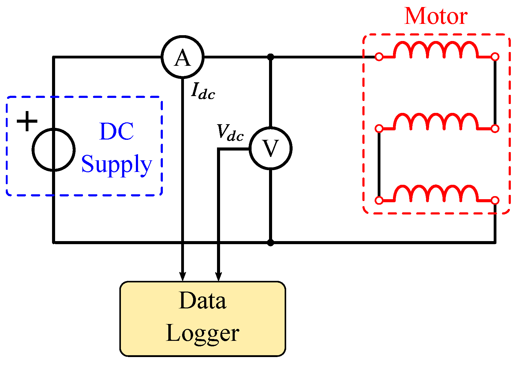
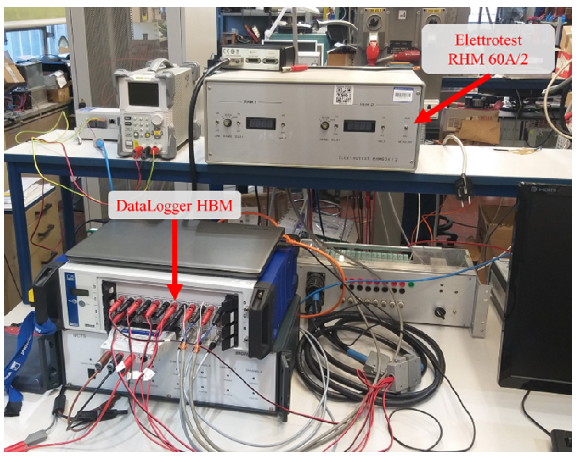
In order to confirm the author’s hypothesis by means of experimental approach, the load test has been repeated, using a specific instrument that can measure the winding resistance injecting a very small DC current while a three-phase motor is running connected to the grid. The used instrument, shown in Figure 8, is an Elettrotest RHM 60A/2 [19]. It is important to underline that the use of the RHM 60A/2 is limited to a sinusoidal supply and it cannot be used with inverter supply.
As shown in Figure 9, a 2-channel resistance meter has been used, with three inlets and three outlets for power supply (for AC decoupling) and two measurement channels (RHM1 and RHM2), each made up of two injection (INJ) and reading (SENSE) terminals. The measure resistance is provided by the external display on the front panel and by an analog signal in the rear panel. The analog signal was used to connect the signal to the data logger HBM Gen4tb. In this way, the complete evolution of the winding resistance can be recorded and consequently its temperature transient.
The results of the new load test are shown in Figure 10 and Figure 11, where it is well evident the excellent agreement between the measured temperatures using RHM60A/2 and the model ones for both the short transients. These results validate the authors’ hypothesis about the time delay introduced by the thermocouple.
It is important to highlight that these results put in evidence as the use of a thermal sensor during temperature transient has to be properly assessed for taking into account its time constant. On the basis of the previous considerations, the temperatures measured using RHM60A/2 has been considered as the reference ones. Figure 12 shows the predicted and the measured by RHM60A/2 temperatures. It is well evident the good agreement between the two curves confirming that the proposed second-order thermal model well predicts the winding temperature both in short and in long thermal transients.

4. Second-Order Thermal Model Improvement

As discussed in Section 3, the second-order thermal model shows good performances both is short transients and steady-state conditions; however, Figure 12 shows discrepancies during the long time transients. The maximum percentage error is around 5% of the measured temperature in the time interval 5 to 6 h. Consequently, a review of the initially proposed has been considered for improving the accuracy of a second-order thermal model. As discussed in Section 2, the thermal resistance R e q , w takes into account the conduction heat transfer between the stator winding and the lamination; however, the stator winding copper can be divided in two sections. The first one is the copper inside the slots (defined as active conductors) and the second one is the copper due to the end winding. The Joule losses due to the active conductors and the end winding can be separated taking into account the geometrical dimensions of the stator stack shown in Figure 13 where D is the average diameter corresponding to the stator slots and L is the stator stack length.
The resistance of a stator winding coil R s , c o i l is proportional to its length due to the length of the active conductors and the coil external connections L c , e c . In first approximation it is possible to write that
R s , c o i l 2 L + 2 L e w = ( 2 L + 2 π D N p )
where N p the number of poles. Let define the shape factor K s as L / D , the ratio between the stator end winding resistance R s , e w and the coil resistance α can be considered proportional to
α = R s , e w R s , c o i l 2 π L N p K s 2 L + 2 π L N p K s = π N p K s 1 + π N p K s
As a consequence, the ratio between the stator end winding Joule losses P e w and the stator total Joule losses P j s can be considered proportional to the coefficient α
P e w P j s = α
The stator end winding losses P e w and the slot copper losses P s l o t can be written as
P e w = α P j s P s l o t = ( 1 α ) P j s
The variation of α versus K s is reported in Figure 14 for different values of the pole numbers N p .
From the thermal point of view, the copper Joule losses of the slot P s l o t move from the slots to the ambient through the stator lamination as shown by the orange arrows in Figure 15. Due to the fins always present in the rotor short circuit rings, the end winding losses move directly from the end winding copper to the frame due to the forced convection effect, as shown by the red arrows of the same figure.
The previously discussed stator Joule losses due to the end winding have been included in an improved second-order thermal model reported in Figure 16. A thermal resistance R e w , a that takes into account the force convection heat exchange of the end winding has been added between the heat source P j s and the ambient temperature T 0 .
The new thermal network is still a second-order thermal model and all the thermal parameters can be measured and computed in easy way. If the value K s is know (from the stator lamination geometrical data) the value of α can be computed by (4) and the value of P e w and P s l o t can be computed by (6). Using the measured values in steady-state condition the value of R e w , a can be computed by
R e w , a = T w T 0 P e w
It is important to underline that the value of the thermal resistance R e q , w can be considered constant, because it takes into account the conduction heat transfer and its value has been obtained using the values measured with DC test. During the DC test the rotor speed is equal to zero and since there is not forced convection heat exchange for the end winding. As a consequence, during the DC test, the thermal resistance R e w , a can be considered equal to infinite and P e w equal to zero. In other words, both the losses P e w and P s l o t are transferred to the ambient by the stator lamination only. On the base of these considerations the computed value of the thermal resistance R e q , w can be considered constant.
The temperatures transients with the new thermal model has been computed using a value of α equal to 0.5 obtained by the design data of the motor under test.
Comparing the results obtained using the original model of Figure 12 and the improved ones of Figure 17 is it evident as the temperatures computed with the improved model better fit the measured ones, even if a discrepancy of 2.1 C (1.61% error) in the steady-state condition at 100% torque can be seen. The response of the improved second-order thermal model is reported in Figure 18 and Figure 19, for the short transient for 0 to 50% and 50% to 100% of the rated torque, respectively. It is well evident the good agreement between the measured and the predicted temperatures in both the transients. In particular, comparing the results shown in Figure 11 and Figure 19 for the transient 50% to 100% is evident the better performance of the improved model with respect to the original one.
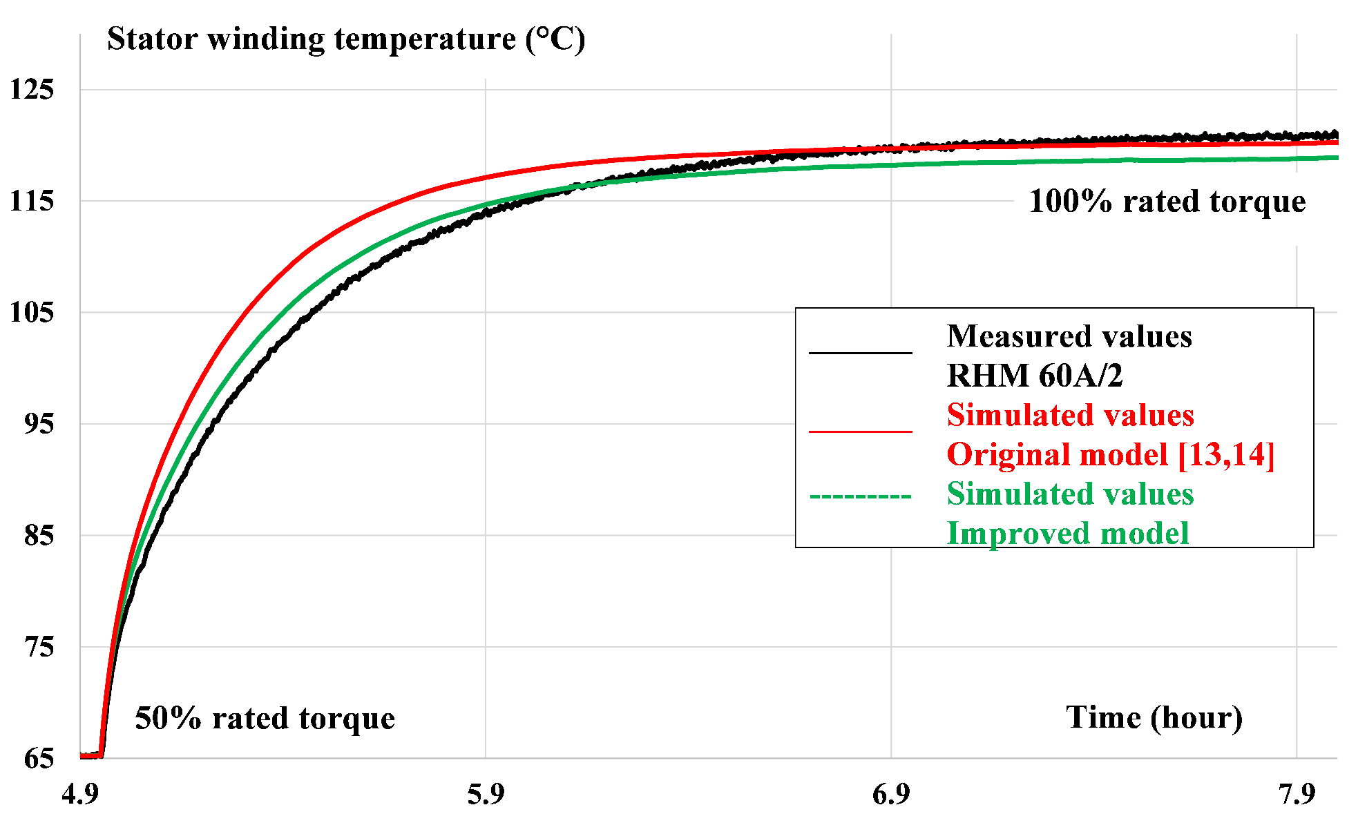
The results obtained with the original model [13,14] and the proposed improved one are highlighted in Figure 20, where the two models have been simulated and compared with the experimental measurements during both thermal transients (50% and 100% of the rated torque). Moreover, to further show the improvement of the proposed model during the thermal transient, a magnification of Figure 20 is available in 
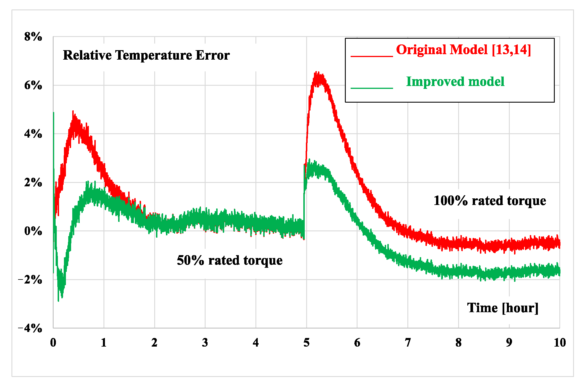
Figure 21, with a focus on the second transient (50% to 100% of the rated torque). The improvement is also quantified in Figure 22, where the relative temperature estimation error is displayed for the original and the improved model. It can be clearly seen that the percentual error during the transient is roughly halved using the proposed model, at the cost of a slightly larger error at steady state. Finally, the thermal parameters of the original model and the improved one are listed in Table 2.

5. Considerations for a Correct Use of the Model

The results discussed in this paper have shown that a second-order model can represent a viable solution for the thermal prediction of an electrical machine in a time interval that starts from a short transient where only the stator winding is involved up to the thermal steady-state condition. Two second-order thermal models have been compared. The first one does not include the forced convection heat exchange in the end winding and shows an excellent accuracy in predicting the steady-state temperature but a worse fitting accuracy during the long temperature transient. The improved model allows and excellent temperature fitting during the long transient but it has a worse accuracy in the prediction of the steady-state temperature. Anyway the maximum temperature errors found in both the models are lower than the 2% and the authors consider this results as an excellent one taking into account how complex is the thermal system and how simple are the proposed models. Even if the proposed second model thermal models have been calibrated and validated on a TEFC induction motor, the models can be used in all the electrical machines with distributed windings taking into account the following considerations.
Electrical machines with natural convection or constant fluid cooling: The proposed models can be used excluding the thermal resistances R f c while R e w , a has to be included in induction motor because the ventilation fins are present in short circuit rings only.
Electrical machines with separated/assisted ventilation (separated/assisted forces convection cooling): The thermal models can be used as they are. R f c is constant because the force convection cooling is constant and does not depend on the rotor speed.
Electrical machines with self ventilation (self-forced convection cooling) (TEFC motors): The model can be uses as they are, but R f c and R e w , a will be depending on the rotor speed. In order to evaluate the variation of the two thermal resistances depending on the motor speed, load tests at different supply frequency have been performed. Since a reduction in the speed corresponds to a reduction in the cooling air speed the load torque has been reduced for avoiding a winding over temperature. The obtained values are reported in Table 3 where is well evident the increase in the thermal resistances values with the reduction in the frequency.
Figure 23 shows the variation of the thermal resistances R f c and R e w , a with the supply frequency. Even if it is possible to find an equation for correlating the values, this equation cannot be considered of general validity. Consequently, the values have to be measured motor by motor. As a final consideration the authors have used a TEFC induction motor for the definition of a second-order thermal model well aware that that motor is the most complex for the thermal point of view. Taking into account that TEFC induction motors are the most complex from the thermal analysis point of view (forced convention on the frame, rotor Joule losses in the cage), the good results obtained on the TEFC induction motor guarantee that the proposed thermal model can be extended to other motor typologies.

6. Conclusions

In this paper, a second-order thermal model is presented and experimental validated. The thermal tests necessary for the thermal parameters determination are analyzed and the procedure to determine them is discussed. Starting from an original second-order thermal model that does not include the cooling effect of the end winding, an improved model that includes these cooling effects has been found and discussed. The advantage of this more accurate model is summarized in a higher accuracy during long transient (i.e., the time interval before reaching the steady-state temperature) at the cost of a slightly lower accuracy at steady-state.
The comparison between the measured and computed winding temperature demonstrates that the proposed second-order thermal models can be considered a simple and accurate approach for predicting the stator winding temperature with an excellent accuracy always lower than 3% both in short transient, long transient and steady-state conditions.

Author Contributions

Conceptualization, A.B., E.C., F.M. and S.R.; methodology, A.B. and E.C.; software, A.B., E.C. and F.M.; validation, F.M. and S.R.; formal analysis, A.B., E.C., M.P. and D.S.; investigation, A.B., E.C., M.P. and D.S.; resources, A.B. and E.C.; data curation, A.B., E.C., F.M. and S.R.; writing—original draft preparation, A.B., F.M. and S.R.; writing—review and editing, A.B., F.M. and S.R.; visualization, A.B., F.M. and S.R.; supervision, A.B. and E.C.; project administration, A.B., E.C., M.P. and D.S.; funding acquisition, A.B., E.C., M.P. and D.S. All authors have read and agreed to the published version of the manuscript.

Funding

This research received no external funding.

Conflicts of Interest

The authors declare no conflict of interest.

Glossary

The following symbols are used in this manuscript:
P J s Stator copper losses
P o l Other machine losses, (iron, rotor Joule losses)
P J s T Stator Joule losses at the temperature T
R e q , w Equivalent thermal resistance between the winding copper and the stator lamination
C e q , w Equivalent thermal capacitance of the winding including copper and insulating material
R e q , s r Equivalent thermal resistance between stator lamination and the ambient
C e q , s r Thermal capacitance of the stator and the rotor not including the stator winding capacitance
R f c Thermal resistance due to forced convection
R e w , a Thermal resistance due to forced convection in the end winding
T w Stator winding temperature
T 0 Ambient temperature
T s r Temperature of the thermal capacitance C e q , s r
WWinding stored thermal energy
Δ T Winding temperature rise
I d c ( t ) DC current sample at the time t
V d c ( t ) DC voltage sample at the time t
tTime
V s Stator voltage
I s Stator current
cos ϕ Stator power factor
TMechanical torque
ω Mechanical speed
P m e c h Mechanical losses
L c , e c Coil external connections length
LStator stack length
DStator lamination length at the middle of the slots
R S , T Phase stator winding resistance at the temperature T
P e l Electrical absorbed power
P i r o n Iron losses
P s l o t Joule losses in the conductors inside the slots
P e w Joule losses in the end winding

References

  1. IEC. IEC 60034-1:2017—Rotating Electrical Machines—Part 1: Rating and Performance; International Electrotechnical Commission: Geneva, Switzerland, 2017. [Google Scholar]
  2. Barlow, T.; Latham, S.; McCrae, I.; Boulter, P. A Reference Book of Driving Cycles for Use in the Measurement of Road Vehicle Emissions; TRL Limited: Berkshire, UK, 2009. [Google Scholar]
  3. Fan, J.; Zhang, C.; Wang, Z.; Dong, Y.; Nino, C.E.; Tariq, A.R.; Strangas, E.G. Thermal Analysis of Permanent Magnet Motor for the Electric Vehicle Application Considering Driving Duty Cycle. IEEE Trans. Magn. 2010, 46, 2493–2496. [Google Scholar] [CrossRef]
  4. Stone, G.; Sasic, M.; Dunn, D.; Culbert, I. Recent problems experienced with motor and generator windings. In Proceedings of the 2009 Record of Conference Papers-Industry Applications Society 56th Annual Petroleum and Chemical Industry Conference, Anaheim, CA, USA, 14–16 September 2009; pp. 1–9. [Google Scholar] [CrossRef]
  5. Barré, O.; Napame, B. The Insulation for Machines Having a High Lifespan Expectancy, Design, Tests and Acceptance Criteria Issues. Machines 2017, 5, 7. [Google Scholar] [CrossRef]
  6. Boglietti, A.; Cavagnino, A.; Staton, D.; Shanel, M.; Mueller, M.; Mejuto, C. Evolution and Modern Approaches for Thermal Analysis of Electrical Machines. IEEE Trans. Ind. Electron. 2009, 56, 871–882. [Google Scholar] [CrossRef] [Green Version]
  7. Kral, C.; Haumer, A.; Bauml, T. Thermal Model and Behavior of a Totally-Enclosed-Water-Cooled Squirrel-Cage Induction Machine for Traction Applications. IEEE Trans. Ind. Electron. 2008, 55, 3555–3565. [Google Scholar] [CrossRef]
  8. Nategh, S.; Huang, Z.; Krings, A.; Wallmark, O.; Leksell, M. Thermal Modeling of Directly Cooled Electric Machines Using Lumped Parameter and Limited CFD Analysis. IEEE Trans. Energy Convers. 2013, 28, 979–990. [Google Scholar] [CrossRef]
  9. Trigeol, J.F.; Bertin, Y.; Lagonotte, P. Thermal modeling of an induction machine through the association of two numerical approaches. IEEE Trans. Energy Convers. 2006, 21, 314–323. [Google Scholar] [CrossRef]
  10. Kral, C.; Haumer, A.; Lee, S.B. A Practical Thermal Model for the Estimation of Permanent Magnet and Stator Winding Temperatures. IEEE Trans. Power Electron. 2014, 29, 455–464. [Google Scholar] [CrossRef]
  11. Sciascera, C.; Giangrande, P.; Papini, L.; Gerada, C.; Galea, M. Analytical Thermal Model for Fast Stator Winding Temperature Prediction. IEEE Trans. Ind. Electron. 2017, 64, 6116–6126. [Google Scholar] [CrossRef]
  12. Jaljal, N.; Trigeol, J.F.; Lagonotte, P. Reduced Thermal Model of an Induction Machine for Real-Time Thermal Monitoring. IEEE Trans. Ind. Electron. 2008, 55, 3535–3542. [Google Scholar] [CrossRef]
  13. Armando, E.; Boglietti, A.; Carpaneto, E.; Rubino, S.; Nair, D.G. Electrical Machines Second Order Thermal Model a Viable Solution for Electric Drives. In Proceedings of the 2020 International Conference on Electrical Machines (ICEM), Gothenburg, Sweden, 23–26 August 2020; Volume 1, pp. 833–839. [Google Scholar] [CrossRef]
  14. Armando, E.; Boglietti, A.; Mandrile, F.; Carpaneto, E.; Rubino, S.; Nair, D.G. Definition and Experimental Validation of a Second-Order Thermal Model for Electrical Machines. IEEE Trans. Ind. Appl. 2021. early access. [Google Scholar] [CrossRef]
  15. Boglietti, A.; Carpaneto, E.; Cossale, M.; Vaschetto, S. Stator-Winding Thermal Models for Short-Time Thermal Transients: Definition and Validation. IEEE Trans. Ind. Electron. 2016, 63, 2713–2721. [Google Scholar] [CrossRef]
  16. Boglietti, A.; Cossale, M.; Vaschetto, S.; Dutra, T. Thermal parameters evaluation for stator fractional-slot concentrated winding machines. In Proceedings of the 2016 IEEE 25th International Symposium on Industrial Electronics (ISIE), Santa Clara, CA, USA, 8–10 June 2016; pp. 228–233. [Google Scholar] [CrossRef]
  17. Boglietti, A.; Cossale, M.; Vaschetto, S.; Dutra, T. Winding Thermal Model for Short-Time Transient: Experimental Validation in Operative Conditions. IEEE Trans. Ind. Appl. 2018, 54, 1312–1319. [Google Scholar] [CrossRef]
  18. IEEE Std 112-2017. IEEE Standard Test Procedure for Polyphase Induction Motors and Generators; Revision of IEEE Std 112-2004; IEEE: Piscataway, NJ, USA, 2017. [Google Scholar] [CrossRef]
  19. Elettrotest. Resistance Meter 60A/2—User Manual; Elettrotest: Badia Polesine, Italy, 2015. [Google Scholar]
Figure 1. Second-order thermal model proposed in [13].
Energies 14 06578 g001
Figure 2. Experimental configuration of the dc test.
Energies 14 06578 g002
Figure 3. Second-order thermal model including the thermal parameter involved with the thermal conduction only.
Energies 14 06578 g003
Figure 4. Steady-state thermal network in load condition.
Energies 14 06578 g004
Figure 5. Comparison between measured and computed winding temperatures.
Energies 14 06578 g005
Figure 6. Comparison between measured and computed winding temperatures during the short transient (0% to 50% of the rated torque).
Energies 14 06578 g006
Figure 7. Comparison between measured and computed winding temperatures during the short transient (50% to 100% of the rated torque).
Energies 14 06578 g007
Figure 8. Instrumentation set up with the HBM DataLogger and the RHM60A/2.
Energies 14 06578 g008
Figure 9. Adopted wiring diagram of the Elettrotest RHM 60A/2 [19].
Energies 14 06578 g009
Figure 10. Comparison between measured (thermal sensor and RHM60A/2) and computed winding temperatures during the short transient (0% to 50% of the rated torque).
Energies 14 06578 g010
Figure 11. Comparison between measured (thermal sensor and RHM60A/2) and computed winding temperatures during the short transient (50% to 100% of the rated torque).
Energies 14 06578 g011
Figure 12. Comparison between measured by RHM60A/2 and computed winding temperatures.
Energies 14 06578 g012
Figure 13. Stator lamination geometrical dimensions.
Energies 14 06578 g013
Figure 14. P e w / P j s vs K s for different values of the pole numbers.
Energies 14 06578 g014
Figure 15. Heat transfer phenomena for the slot copper (orange arrows) and the end windings (red arrows).
Energies 14 06578 g015
Figure 16. Improved second-order thermal model.
Energies 14 06578 g016
Figure 17. Comparison between measured and predicted winding temperature using the improved second-order thermal model.
Energies 14 06578 g017
Figure 18. Comparison between measured (RHM60A/2) and computed winding temperatures during the short transient (0% to 50% of the rated torque) using the improved second-order thermal model.
Energies 14 06578 g018
Figure 19. Comparison between measured (RHM60A/2) and computed winding temperatures during the short transient (50% to 100% of the rated torque) using the improved second-order thermal model.
Energies 14 06578 g019
Figure 20. Comparison between measured (RHM60A/2) and computed winding temperatures during the whole test using the original [13,14] and the improved second-order thermal model.
Energies 14 06578 g020
Figure 21. Comparison between measured (RHM60A/2) and computed winding temperatures during the long transient (50% to 100% of the rated torque) using the original [13,14] and the improved second-order thermal model.
Energies 14 06578 g021
Figure 22. Relative temperature estimation error during the thermal test of the original [13,14] and the improved second-order thermal model.
Energies 14 06578 g022
Figure 23. Thermal resistances R f c and R e w , a values vs. supply frequency.
Energies 14 06578 g023
Table 1. Considered TEFC motor data.
Rated Power (kW)4
Rated Voltage (V)400
Rated Frequency (Hz)50
Rated Current (A)8.8
Pole Pairs2
Rated Speed (rpm)1410
Table 2. Parameters table for the standard model of [13,14] and the proposed model.
ParameterStandard Model [13,14]Proposed Model
R e q , w (K/W)0.070.07
C e q , w (J/K)1708.21708.2
C e q , s r (J/K)10,85710,857
R e q , s r (K/W)0.3820.382
R f c (K/W)0.08600.167
R e w , a (K/W)-0.446
Table 3. Variation of R f c and R e w , a and with the supply frequency.
Frequency (Hz)Torque (%)Speed (rpm)Rotor Surface
Speed (m/s)
R fc (°C/W) R ew , a (°C/W)
10652202.240.9600.729
20505655.750.3340.527
30508668.810.2260.496
4070114711.680.1890.481
50100140214.270.1670.446
Publisher’s Note: MDPI stays neutral with regard to jurisdictional claims in published maps and institutional affiliations.

