Lumped-Parameters Thermal Network of PM Synchronous Machines for Automotive Brake-by-Wire Systems

Abstract

Thermal analysis represents a key factor in electrical machine design due to the impact of temperature increase on insulation lifetime. In this context, there has been a wide investigation on thermal modeling, particularly for machines used in harsh working conditions. In this perspective, brake-by-wire (BBW) systems represent one of the most challenging applications for electrical machines used for automotive smart actuators. Indeed, electro-actuated braking systems are required to repeatedly operate the electric machine in high overload conditions in order to limit the actuator response time, as well as to enhance gravimetric and volumetric specific performance indexes. Moreover, BBW systems often impose unconventional supply conditions to the electric machine, consisting of dc currents in three-phase windings to keep the rotor fixed during the braking intervals. However, a dc supply leads to uneven temperature distributions in the machine, and simplified thermal models may not accurately represent the temperature variations for the different machine parts. Considering such unconventional supply conditions, this paper initially investigates the applicability of a conventional lumped-parameters thermal network (LPTN) based on symmetry assumptions for the heat paths and suitable for surface-mounted PM synchronous machines used in BBW systems. An extensive test campaign consisting of pulses and load cycle tests representative of the real machine operations was conducted on a prototype equipped with several temperature sensors. The comparison between measurements and predicted average temperatures, together with insights on the unbalanced heat distribution under the dc supply obtained by means of finite element analyses (FEA), paved the way for the proposal of a phase-split LPTN with optimized parameters. The paper also includes a critical analysis of the optimized parameters, proposing a simplified, phase-split lumped-parameters thermal model suitable to predict the temperature variations in the different machine parts for PM synchronous electric machines used in BBW systems.

1. Introduction

Permanent magnet synchronous machines (PMSMs) are nowadays widely used in the automotive industry for the electrification of smart actuators. Indeed, their superior torque and power density values outweigh the drawback of high costs for rare-earth permanent magnets usually adopted to achieve such enhanced specific indexes. However, the challenging targets imposed by the automotive industry for weight and dimensions of auxiliary systems often require exploiting to the maximum extent the overload capabilities granted by electric drives. In some cases, overload working conditions may even represent the normal operation for electric machines that actuate intermittent duty auxiliaries. Therefore, a tight thermal and electromagnetic modeling is mandatory from the early design stage of these power-dense components to guarantee both the target output power as well as the required device lifetime and reliability.

In fact, severe overloads together with harsh environmental conditions may result in overtemperatures that can exceed the thermal limits of the electric machine. The importance of operation within the safe temperature range is even more exacerbated for electric machines used in critical components for the vehicle and passengers’ safety, such as brake-by-wire (BBW) systems [1]. Electric braking is a cutting-edge technology in which the traditional hydraulic brake architecture is substituted by electro-actuated braking systems supplied at 12 or 48 V. In addition to dimension and weight constraints, the electric machines used in these actuators are also operated in overload conditions to limit the brake response time and, consequently, the vehicle braking distance.

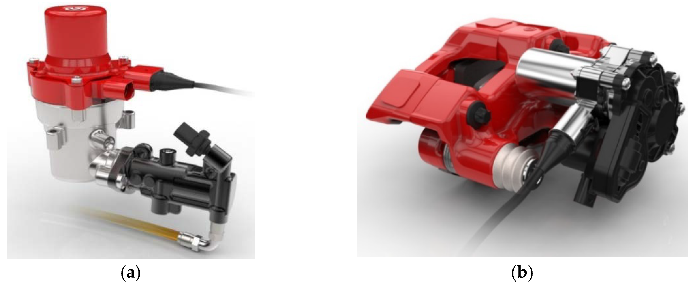
Different BBW solutions are possible depending on the caliper actuation system. For instance, Figure 1a shows an electro-hydraulic solution that converts electric energy into hydraulic pressure to actuate a standard brake caliper, while Figure 1b shows an electromechanical brake caliper in which electric energy is directly converted into clamping force [2]. The three-phase electric machine used for the electro-hydraulic and electromechanical brake is for most of the working time supplied by a dc current to keep the rotor in a fixed position during the braking intervals. A dc current supply results in a non-uniform temperature distribution in the machine because of the unbalanced current flow in the three phases. Therefore, conventional lumped-parameters thermal models based on circumferential symmetry assumptions for the heat paths may not properly predict the temperature variation for the different machine parts during the real operation.

This paper investigates the use of lumped-parameters thermal networks (LPTNs) for predicting the temperature evolution in operative conditions of PM synchronous machines used in automotive BBW systems. In detail, the study focuses on the electric machine for electromechanical brake calipers (see Figure 1b). A conventional high-order LPTN that considers symmetrical heat paths was initially calibrated and used to replicate test conditions at different dc current levels and load cycles representative of real operations. The predicted temperature evolutions were compared with measurements executed on a prototype equipped with several thermal sensors. By the investigation of the heat paths in the machine with finite element analyses (FEAs), ‘asymmetrical’ LPTNs were proposed to closely match the temperature evolution for each stator winding phase and all the machine parts, both for the test conditions and the operative load cycles.

2. Lumped-Parameters Thermal Models for PM Synchronous Machines

The literature reports a considerable number of research papers that focus on thermal analysis of electric machines. Depending on the analysis techniques used to compute the temperature distribution, thermal models can be mainly categorized as (1) analytical and (2) numerical models [3,4,5]. Both modeling methods feature advantages and drawbacks that impact on the thermal model complexity, accuracy, and resolution time [6,7].

Sometimes, experimental component modeling on motorette samples is also used to calibrate analytical and numerical electric machine models [3,8,9,10,11]. This approach unquestionably allows the modeling accuracy to increase, but time and budget for sample realization have to be properly considered.

Numerical models consist of thermal FEA or computational fluid dynamic (CFD) models that allow accurate prediction of the temperatures in the different machine parts [12,13,14,15]. However, detailed knowledge of the machine’s geometrical dimensions and the characteristics of the used materials is mandatory, as well as knowledge of the details of the cooling system. Moreover, the model setup as well as its resolution are usually very time consuming. Because of these drawbacks, engineers working in manufacturing companies often limit numerical thermal analyses only to the final design stage, occasionally using multiphysics models for a comprehensive performance assessment of the electric machines [16,17]. Sometimes, electromagnetic and thermal numerical co-simulations are conducted to assess faulty conditions [18].

Analytical thermal models consist of lumped-parameters networks modeled on the basis of the heat transfer theory [19,20]. This approach exploits the modeling equivalence between thermal and electric circuits. In detail, thermal resistances represent the heat transfer due to conduction, convection, and radiation phenomena and allow computation of the steady-state temperatures, while thermal capacitances represent the energy storage capacity and allow modeling of the thermal transient behavior. In the thermal network, the heat sources related to the different machine losses are modeled by means of current generators, while the node voltages represent the temperature values for the different machine parts. Obviously, the lumped nature of this modeling approach considers each machine loss and the corresponding heat source as uniformly distributed into the machine components [21]. Similarly, the node voltages represent the average temperatures for the modeled machine parts. Increasing the number of nodes results in a higher-order thermal network that better discretizes the machine under analysis but at the expense of increased model complexity because of the larger number of parameters that have to be determined.

The parameter values of the LPTN can be mainly computed using equations reported in literature upon the knowledge of machine dimensions and material properties [19]. In detail, thermal capacitances are derived by the weight and the specific heat capacity of the materials, while thermal resistances are usually determined assuming the different machine parts as hollow cylinders. The heat transfer coefficients due to radiation and convection are typically obtained by empirical formulas [22,23,24,25]. However, for particularly complex and high-order LPTNs, as well as for those cases where the assumptions for the thermal parameters computations are not rigorous, the identification of a thermal parameters set that allows accurate replication of the temperature variations measured on the real machine may not be straightforward. In these cases, optimization techniques are often used in conjunction with measurements to properly calibrate the thermal network parameters [26,27,28,29,30]. Nevertheless, complex LPTNs are often simplified considering only the main heat paths, both for more straightforward parameters identification as well as to make the LPTN suitable for online temperature predictions during machine operation [31].

The analytical computation of some thermal network parameters is not trivial. For instance, the computation of the thermal resistance between stator copper and stator core has to consider a heat path through an agglomerate of multiple materials with different thermal properties, while the thermal resistance between machine housing and the ambient areas comprises both convection and radiation phenomena. The literature reports dc tests that allow the calibration of such parameters [8,10,24,32]. It is interesting to observe that, even though for most of the applications those dc tests represent ‘ad hoc’ calibrating procedures, for the electric machine analyzed in this paper such supply conditions were also representative of the real machine operations.

Papers based either on analytical or numerical approaches for thermal models of PM synchronous machines can be found in literature. In particular, recent research works propose multidimensional analytical thermal models to consider additional heat paths with respect to the one-dimensional (1-D) heat flow modeled through a thermal resistance. For instance, in [5,23], two-dimensional analytical thermal models are proposed for PM machines, while in [18,26], three-dimensional analytical thermal approaches are proposed for predicting the temperature in synchronous machines affected by faults in the stator winding. Regardless of the model complexity, optimization techniques are usually adopted in literature to identify a suitable set of values for the network parameters [27,31]. Moreover, simplifying assumptions are often introduced to reduce network complexity and to get an easy-to-handle model while preserving the required accuracy [31,33].

Differently from the solutions proposed up today in literature, this paper proposes the use of conventional one-dimensional LPTNs for predicting the temperature variation in PM synchronous machines when a dc supply is provided to the stator winding. As articulated in the paper, the unbalanced heat distribution under such supply conditions is considered, modeling the thermal behavior of each stator phase independently.

3. Thermal Tests for Model Definition

The electric motor of the electromechanical actuator under analysis is a surface permanent magnet (SPM) three-phase motor with double-layer fractional slot concentrated windings. During real operations, the braking is provided by the motor by injecting repetitive dc currents in two of the three phases of the stator. The machine under test was equipped with several thermocouples positioned in the slots, internally to the coils, and on the external housing.

In order to assess the thermal performances of the motor, several thermal tests were conducted. For these tests, two different setups were used. For one test setup, the motor was placed on a plastic support and cooled by natural air, as shown in Figure 2a. This setup was used to perform the pulse tests on the motor. The definition of a pulse test is given later on. For the other test setup, the motor was inserted in a climatic chamber to keep the ambient temperature close to the hypothetic working ambient temperature of 120 °C, as depicted in Figure 2b. This setup was used to perform load cycle tests on the motor with the aim of emulating the real working conditions of the actuator.

The performed tests can be grouped into pulse tests and load cycle tests. A pulse test consists of injecting a dc current into the stator winding until the maximum admissible temperature is reached. In some cases, when low values of dc currents are injected in the motor, the maximum temperature is never reached and, therefore, the pulse duration is arbitrary; these tests are considered as steady-state tests.

The injection of a dc current in a three-phase star-connected winding with a non-accessible common point is feasible in two different ways. The two configurations that allow such supply are shown in Figure 3 and referred to here as configuration A (Figure 3a) and configuration B (Figure 3b).

In total, 20 tests were performed. In particular, 18 were pulse tests, performed for different current values and using the two different configurations. In detail, half of them were performed in configuration A, while the other half were in configuration B. The remaining two tests were braking cycles tests that emulated the real working conditions of the motor. During the tests, temperatures in different machine parts were measured thanks to the embedded thermal sensors, while the thermal power dissipated by the machine was determined by the product of the injected dc current and voltage. The thermocouples used had an accuracy of ±0.75%, while the dc voltages and currents were measured with an accuracy equal to 0.02%. 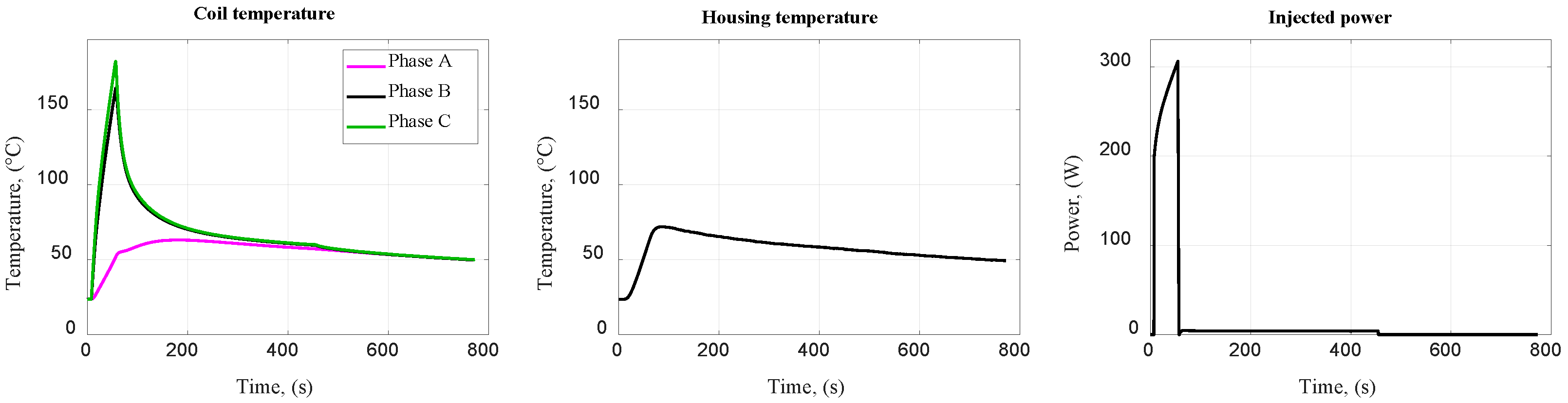Some representative measurements are reported in Figure 4, Figure 5 and Figure 6. In Figure 4, the obtained measurements for a long-time duration of dc current injection and the stator winding connections in configuration A are shown. 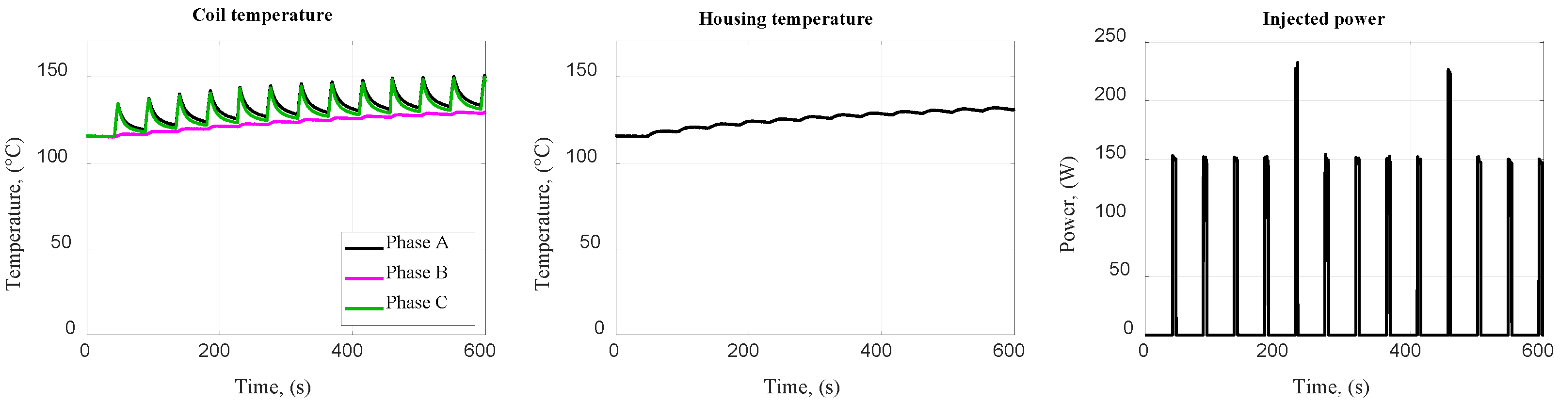Figure 5 depicts the obtained measurements in the same configuration but for a short time dc current pulse, while Figure 6 shows the measurements of one of the two load cycles. As expected, with configuration A, the phase with no supply was colder than the other two. Vice versa, in configuration B, the phase that carried the whole current was hotter than the other two.

Table 1. Summary of the conducted thermal tests.

Test Name	No. of Tests	Test Setup	Phase A	Phase B	Phase C
Pulses A	9	Ambient air	C	H	H
Pulses B	9	Ambient air	C	H	C
Cycle 1	1	Climatic chamber	H	H	C
Cycle 2	1	Climatic chamber	H	C	H

summarizes all the performed tests, by specifying the number of conducted tests for each test topology, the ambient in which the motor was located and which phase was ‘hot’ (H) or ‘cold’ (C). In particular, pulses tests that are used to calibrate and validate the proposed thermal models were conducted at ambient temperature, while load cycle tests that were representative of the real working conditions of the actuator were conducted in the climatic chamber to emulate the ambient temperature during the operation on the vehicle.

4. Conventional Lumped-Parameters Thermal Network

At first, a conventional lumped-parameters thermal network of the fifth order was developed to predict the temperatures of the different parts of the motor, among them the winding temperature and the housing temperature, in order to make a comparison with the measurements. The LPTN was initially proposed by the authors in [29] and adapted here for the specific application. The machine was subdivided into several parts that were assumed to have the same thermal behavior. In particular, the motor was subdivided into hollow cylinders concentric with the rotor axis [34]. The hypotheses at the base of the developed thermal model were as follows:

• the motor was symmetrical around the shaft and about the radial plane through the center of the machine;
• the influence of the uneven temperature distribution was neglected;
• each cylinder was thermally symmetrical in the radial direction;
• the heat sources were uniformly distributed;
• the heat flux in the axial direction was considered only in the shaft.

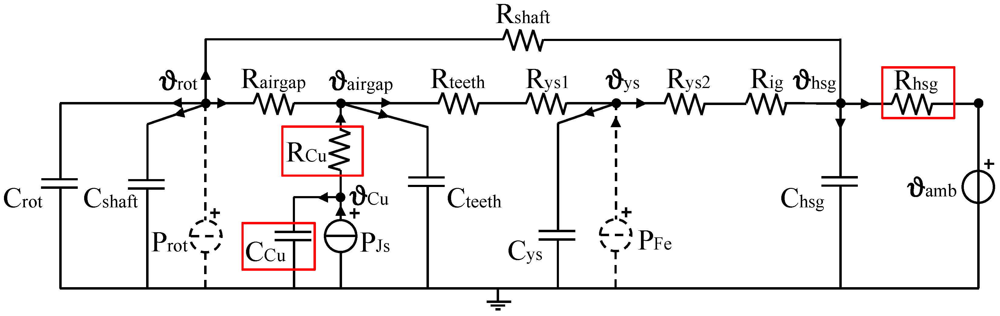
The LPTN allowed the prediction of the main motor temperatures, and it is depicted in Figure 7. The considered temperatures were ${\vartheta }_{rot},$ the temperature of the rotor; ${\vartheta }_{airgap},$ the temperature of the air gap;${\vartheta }_{Cu},$ the temperature of the stator winding; ${\vartheta }_{ys},$ the temperature of the stator yoke; ${\vartheta }_{hsg},$ the temperature of the housing. With respect to a conventional LTPN of the fifth order, the losses on the rotor and the losses in the stator iron were neglected and, therefore, represented with a dashed line. Indeed, since the motor works in dc, the only loss sources to be considered in the model were the Joule losses (P_Js), as happens in the considered BBW application.

All the parameters of the LPTN were computed by means of the dimensions of the motor and the thermal characteristics of the used materials, except for the thermal resistance of the housing and the parameters relative to the stator winding, which are all represented in red squares in Figure 7. These parameters were calibrated on the dc test with the lowest current in configuration A.

In particular, the value of R_hsg was computed by dividing the steady-state value of the housing overtemperature by the injected power. For the values of R_cu and C_cu, an optimization algorithm was used and applied only for the first instants of transient thermal analysis, when the winding heating can be considered adiabatic. Hence, a thermal model of the first order could be used to determine the R_cu and C_cu parameters. This was accomplished by optimization, searching for a good match between the computed and measured temperatures. In particular, the average temperature between phase B and phase C of the steady state test in configuration A (Figure 4, left) was considered.

The value of the obtained thermal resistance was 0.61 °C/W, while the value of the thermal capacitance was 38.7 J/°C. However, the values of the parameters identified thanks to the first-order adiabatic thermal model could not be directly used in the network shown in Figure 7 because in configuration A only two phases stored thermal energy. Consequently, the value of the thermal resistance had to be multiplied by 2/3, while the value of the capacitance was multiplied by 3/2.

The final values are reported in

Table 2. Computed and calibrated thermal parameters.

Parameter	Symbol	Value	Unit
Rotor yoke and PM capacitance	Crot	49.5	J/°C
Shaft capacitance	Cshaft	15.7	J/°C
Stator winding capacitance	CCu	58	J/°C
Stator teeth capacitance	Cteeth	31	J/°C
Stator yoke capacitance	Cys	41	J/°C
Housing capacitance	Chsg	46	J/°C
Shaft resistance	Rshaft	10.5	°C/W
Airgap resistance	Rairgap	6.3	°C/W
Stator winding–core resistance	RCu	0.4	°C/W
Stator teeth resistance	Rteeth	0.07	°C/W
Inner stator yoke resistance	Rys1	0.004	°C/W
Outer stator yoke resistance	Rys1	0.004	°C/W
Stator yoke–housing interface gap resistance	Rig	0.12	°C/W
Housing–ambient resistance (setup Figure 2a)	Rhsg	3.9	°C/W
Housing–ambient resistance (setup Figure 2b)	Rhsg	0.66	°C/W

, along with all the other computed parameters. With respect to the housing–ambient thermal resistance with the setup shown in Figure 2b, the pulse test in steady-state condition was not performed. Then the value was set to 0.66 °C/W in accordance with the optimization results reported in Table 3.

The measured ambient temperature and the injected power were given as input to the LPTN of Figure 7. The predicted temperatures were obtained by solving the differential equations listed in Equation (1). A simple method of Euler was used to solve the system, since no challenging dynamics were involved.

$$\{\begin{array}{c}\frac{d{\vartheta }_{rot}}{dt}=\frac{{\vartheta }_{airgap}-{\vartheta }_{rot}}{C_{rot}·R_{airgap}}+\frac{{\vartheta }_a-{\vartheta }_{rot}}{C_{rot}·R_{Shaft}}\hfill \\ \frac{d{\vartheta }_{Cu}}{dt}=\frac{P_{Js}}{C_{Cu}}+\frac{{\vartheta }_{airgap}-{\vartheta }_{Cu}}{C_{Cu}·R_{Cu}}\hfill \\ \frac{d{\vartheta }_{airgap}}{dt}=\frac{{\vartheta }_{ys}-{\vartheta }_{airgap}}{C_{teeth}·\left(R_{teeth}+R_{ys1}\right)}+\frac{{\vartheta }_{Cu}-{\vartheta }_{airgap}}{C_{teeth}·R_{Cu}}+\frac{{\vartheta }_{rot}-{\vartheta }_{airgap}}{C_{teeth}·R_{airgap}}\hfill \\ \frac{d{\vartheta }_{ys}}{dt}=\frac{{\vartheta }_{airgap}-{\vartheta }_{ys}}{C_{ys}·\left(R_{teeth}+R_{ys1}\right)}+\frac{{\vartheta }_{hsg}-{\vartheta }_{ys}}{C_{ys}·\left(R_{ys2}+R_{ig}\right)}\hfill \\ \frac{d{\vartheta }_{hsg}}{dt}=\frac{{\vartheta }_{ys}-{\vartheta }_{hsg}}{C_{hsg}·\left(R_{ys2}+R_{ig}\right)}+\frac{{\vartheta }_a-{\vartheta }_{hsg}}{C_{hsg}·R_{hsg}}\hfill \end{array}$$

(1)

All the performed tests were simulated through the LPTN of Figure 7. However, for the sake of simplicity, only the results for some selected tests are hereafter reported as representative of the performance of the network.

In Figure 8 and Figure 9, the computed temperatures for the long-time pulse tests are reported, for configuration A and B, respectively, while in Figure 10 and Figure 11, the results for the short-time pulse tests are shown. As can be seen, the predicted temperatures matched well with the measured ones, both for the housing and the winding. Therefore, the conventional LPTN already represents a reliable model to estimate the motor temperatures. However, it is not reasonable to compare the computed average temperature of the three-phase winding with the temperatures measured on each phase. It seems that, for all the tests, the computed winding temperature predicted the hottest phase(s). This is even more evident for the load cycle tests.

In Figure 12 and Figure 13, the measured and the computed temperatures for the two load cycles are reported. The obtained results showed less accuracy in comparison with the pulse tests’ results, even if the R_hsg was adjusted as indicated in Table 2, when the machine was inside the climatic chamber. On the basis of the obtained results, the definition of an LPTN that can predict the temperatures of the three phases distinctly may be a worthy improvement for this kind of application. In order to develop such an LPTN, a preliminary investigation on the unbalanced heating of the machine was carried out. For this reason, a finite element model of the motor was created and supplied with different values of Joule losses on the three phases.

5. Finite Element Analysis of Unbalanced Heat Distribution

The real operating conditions of this machine under dc supply resulted in a non-uniform temperature distribution. A difference in the temperatures of each phase was already evident in the measurements. Nevertheless, a transient 2D thermal finite element model with a second-order mesh having around 270,000 elements was built, in order to further understand the effect of the uneven supply on the temperature distribution on the whole machine geometry. The model considered all the electro-magnetic active parts of the machine, including the copper insulation, as well as the liner and the impregnation. The governing equations of the thermal model are presented in Appendix A, together with more implementation details about the FEM model.

Each material was defined by an isotropic constant thermal conductivity value and a volumetric heat capacity value. The thermal exchange between the machine and the surrounding fluid was defined by means of a convection boundary condition on the external housing. In particular, the related convection thermal was computed starting from the value of R_hsg as indicated in Equation (2), where $A$ is the lateral external surface of the housing.

$$h=\frac{1}{R_{hsg}·A}$$

(2)

The measured injected power in each phase was given as the input to the corresponding phase region in the finite element model.

Figure 14 shows the comparison between the FEA-computed temperatures and the measured ones for the lowest current value in configuration A. The winding temperatures were the average value on the region surface relative to each phase, while the housing temperature was the average value computed on the external circumference of the housing. The FEA-predicted temperatures showed a good accuracy when compared to the measurements. Hence, the finite element model represented a reliable model to predict the temperatures of the three phases as well as the temperature of the housing, although a higher complexity for the model setting and longer computational time were required in comparison to an LPTN.

In Figure 15, the color shade maps of the temperature distributions are shown. In particular, the selected instant corresponds to the highest values reached by the temperatures. Figure 15a shows the temperature distribution for configuration A, while Figure 15b shows the same for configuration B. In both cases, all the lines of the motor geometry and the rotor structures were deleted in order not to share sensitive content. However, the rotor was substantially isothermal. The ambient temperature of both simulations was the same and equaled 24.4 °C, while the injected powers were different. By looking at Figure 15, the unbalanced temperature distribution is well evident. In detail, configuration A presented a more uneven temperature distribution with respect to configuration B. In order to reproduce such conditions with a lumped-parameter thermal network, the branch relative to the stator winding had to be split into three and supplied with the corresponding power. Moreover, new thermal paths may be reasonable to consider: a possible heat exchange among the three phases and a heat exchange with the housing through the end winding. In the light of this analysis, an improved LPTN was developed and is discussed in Section 6.

6. The Phase-Split Lumped-Parameters Thermal Network

Initially, a lumped-parameters thermal network where the three phases were split was proposed in order to consider the non-homogeneous heating of the machine. The new model is presented in Figure 16. In this version, the winding equivalent thermal resistance (previously referred as R_Cu) was split in three different branches of thermal resistance, R₁. Furthermore, a heat exchange among the three phases was considered by adding the three thermal resistances, R_x. Finally, the three parameters of value R_y introduced an additional heat path representing the heat exchange between the end winding and the housing. The new structure of the network allowed the three phases to be supplied independently. The temperatures in the different nodes of the phase-split LPTN were computed by solving the corresponding system of differential equations and by using the method of Euler since no fast dynamics were involved.

In this new network, the parameters were unknown, and they could not be computed by means of dimensions of the motor and the thermal characteristics of the used materials, since the hypothesis of motor symmetry was not applicable anymore. For this reason, an optimization algorithm was used to find the parameters.

6.1. Optimization Algorithm for the Identification of the Thermal Parameters

The values of the thermal parameters were found by using particle swarm optimization (PSO). The objective function of the optimization was the quadratic error in Equation (3). To define such a function, for each test, for each temperature, and for each time instant, the quadratic error between the measured and computed temperature was computed. These values were summed up for the whole duration of each test and for the four temperatures (three coil temperatures and the housing). The final function was obtained by summing up the quadratic error of all the tests.

$$E={\displaystyle \sum }_{j=1}^{n_{test}}{\displaystyle \sum }_{i=1}^{n_{\vartheta }}{\displaystyle \sum }_{z=0}^Z{\left({\vartheta }_{measure{d}_{i,z}}^j-{\vartheta }_{compute{d}_{i,z}}^j\right)}^2$$

(3)

In this function,

• j is the index that indicates the j-th thermal test ($n_{test}\le 20$ is the number of tests considered for optimization purposes);
• i is the index that indicates the temperatures of the considered machine parts ($n_{\vartheta }\le 4$ is the number of monitored machine parts);
• z is the index that indicates the considered temperature samples ($Z$ is the number of considered samples of the considered thermal test).

Several optimizations with PSO were performed, varying $n_{test}$ and $n_{\vartheta }$. All the results showed that some parameters, such as R_x, assumed very high values, meaning that an optimized network for the considered machine structure with fractional-slot concentrated winding layout should not consider that specific heat path; other parameters seemed to not have a significant impact on the results. As a consequence, the critical analysis of the optimized parameters led to the finding that the network shown in Figure 16 can be suitably simplified, as discussed hereafter.

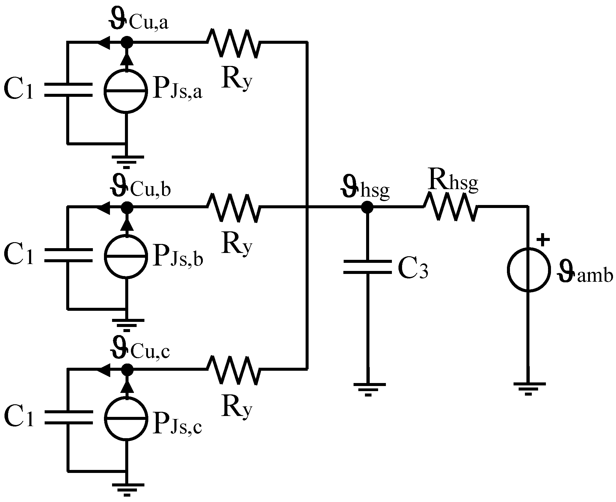
6.2. The Simplified Phase-Split Lumped-Parameters Thermal Network

In Figure 17, the optimized thermal network is shown and, as can be seen, the four nodes allow the computation of the four considered temperatures. Once again, the values of the parameters were obtained by means of PSO. It must be recalled that the two load cycle tests took place in a climatic chamber and that this has an impact on the value of the parameters, especially on R_hsg. For this reason, two distinct optimizations were needed: one for the pulse tests ($n_{test}$ = 18 and $n_{\vartheta }$ = 4) and one for the cycle tests ($n_{test}$ = 2 and $n_{\vartheta }$ = 4). The obtained parameters are listed in Table 3.

Table 3. Optimal thermal parameters of the simplified phase-split LPTN.

Parameter	Pulses	Cycles
C1	22 J/°C	22 J/°C
C3	220 J/°C	220 J/°C
Ry	1.16 °C/W	0.68 °C/W
Rhsg	3.9 °C/W	0.66 °C/W

Table 3. Optimal thermal parameters of the simplified phase-split LPTN.

Parameter	Pulses	Cycles
C1	22 J/°C	22 J/°C
C3	220 J/°C	220 J/°C
Ry	1.16 °C/W	0.68 °C/W
Rhsg	3.9 °C/W	0.66 °C/W

Looking at the table, the same values of thermal capacitances were obtained for both optimizations. This is reasonable since these values only depend on the specific heat of the materials and on their weight. It is interesting to point out that the sum of the four thermal capacitances obtained by the present optimization (242 J/°C) is very close to the sum of all the thermal capacitances of the conventional LPTN of Figure 7 (241.2 J/°C). Furthermore, it was verified that the thermal capacitance of the three-phase winding (C_Cu = 58 J/°C, computed by the adiabatic first-order thermal model) was about three times the capacitance, C₁, extracted by optimizing the simplified phase-split LPTN.

The difference in the thermal resistances between the pulse tests and the cycle tests might have been due to the different test setups and ambient temperatures, particularly for the thermal resistance that represents the heat exchange with the ambient.

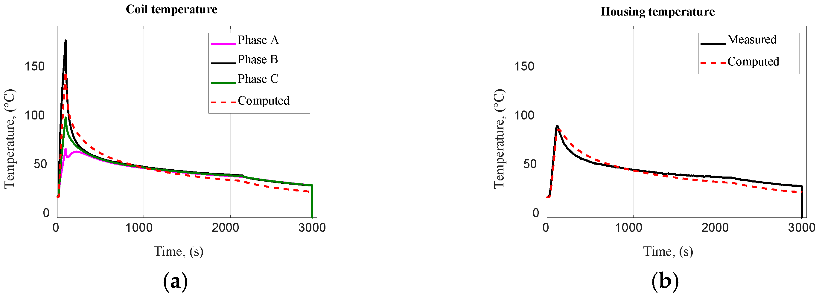
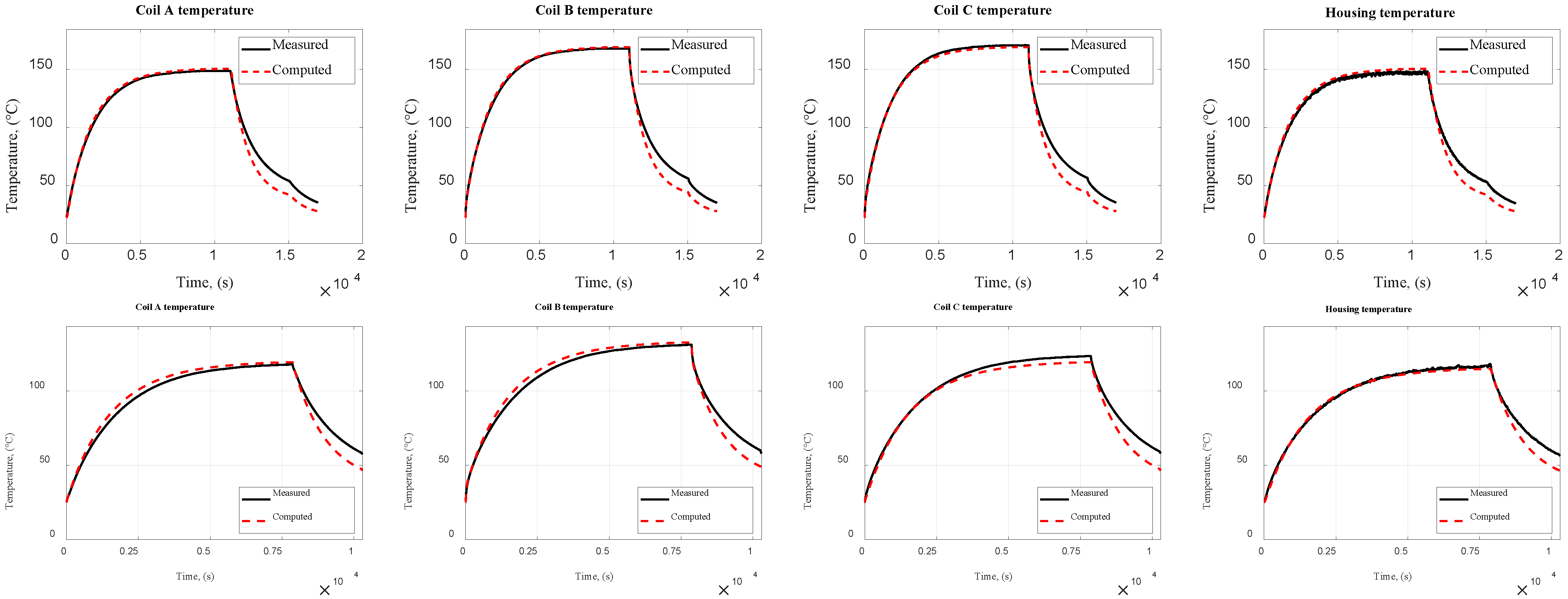
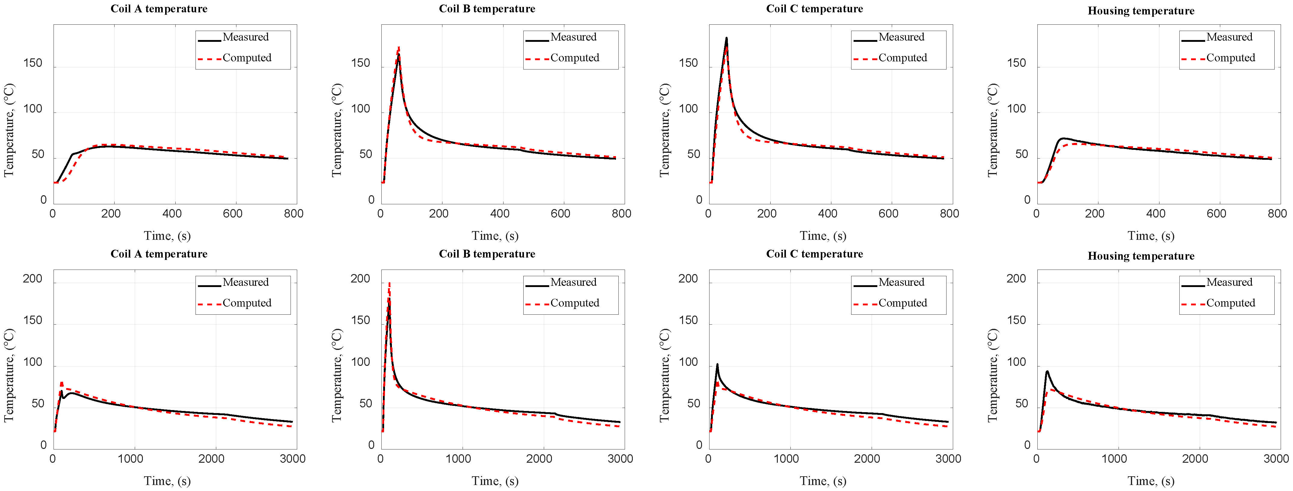
6.3. Comparison between Computed and Measured Temperature Trends

Some selected results are presented with the aim of showing the potentiality of the proposed simplified thermal network, which effectively allows the prediction of the temperature of each phase with high accuracy, considering the unconventional supply conditions imposed by the BBW application.

Figure 18 and Figure 19 show the results for long-time and short-time pulse tests, in both A and B stator winding configurations, proving the goodness of the proposed simplified phase-split LPTN. The results’ goodness can also be appreciated by the percentage errors between computed and measured temperatures for long-time pulse tests, both for configuration A and B, listed in

Table 4. Percentage errors for the long-time pulse tests shown in Figure 8, Figure 9 and Figure 18 (evaluated at the end of the dc power pulse as error = 100 × (T_computed − T_measured)/T_measured).

Motor Parts	Configuration A		Configuration B
	Conventional Model	Phase-Split Model	Conventional Model	Phase-Split Model
Phase A	+14.5%	+1.2%	+9.4%	+1.3%
Phase B	+1.4%	+0.8%	−1.7%	+1.2%
Phase C	−0.3%	−0.9%	+4.5%	−3.3%
Housing	+1.8%	+1.8%	−1.4%	−1.4%

. As expected, the conventional and the simplified phase-split LPTNs provided comparable results for the two hot phases and the housing, while for the cold phase, a better fit was obtained by the proposed phase-split model.

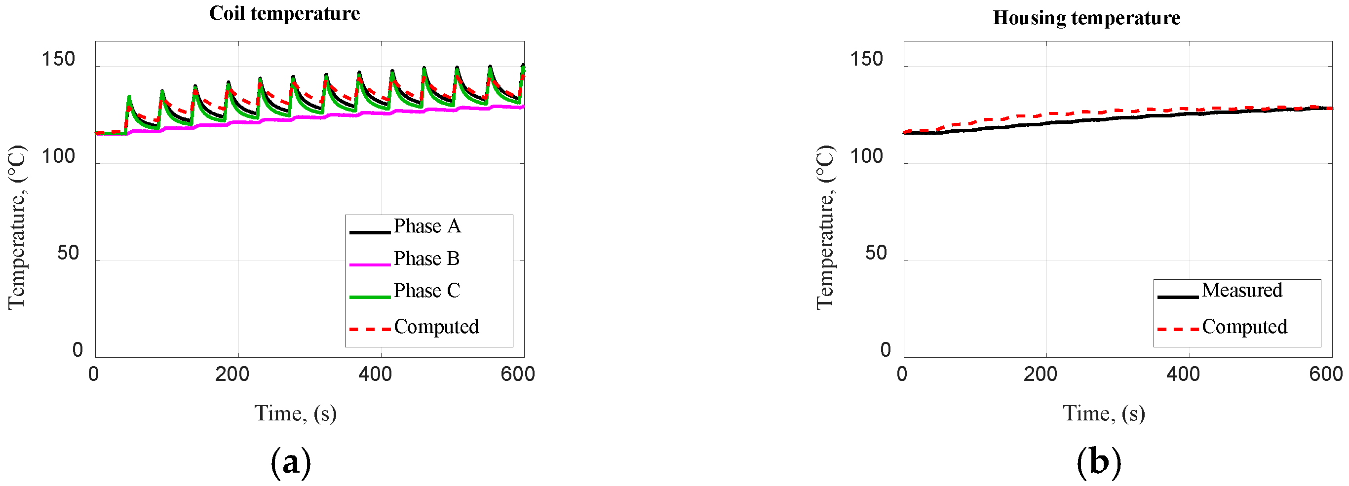
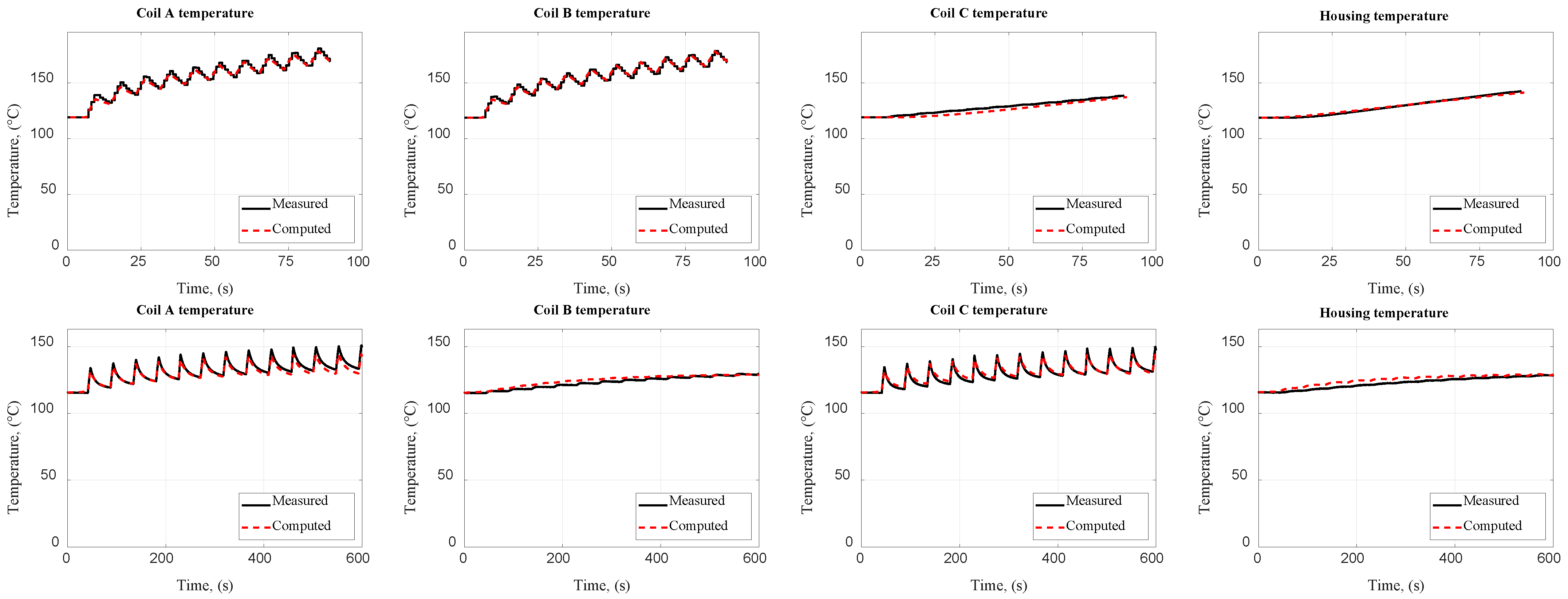
Very good agreements between measured and computed temperatures were also obtained for the ‘hot’ and ‘cold’ phases in the load cycle tests, as depicted in Figure 20.

7. Conclusions

This paper presents a phase-split lumped-parameters thermal network that allows the prediction of the temperatures of the three phases and of the housing of an SPM motor with double-layer fractional slot concentrated windings used in an electromechanical brake-by-wire system. The application requires unconventional supply conditions for the motor, specifically continuous currents that are repetitively injected in two of the three phases of the stator winding, with the aim of braking. This supply condition leads to an uneven heating of the motor and especially to different values of the three phases’ temperatures.

An extensive thermal test campaign was conducted. The motor was tested with two categories of thermal tests: pulse tests and load cycle tests. The pulse tests consisted of injecting a dc current into the stator winding until the maximum admissible temperature was reached. Different values of currents were tested, with two different configurations of the stator winding. The load cycle tests were braking cycles tests that emulated the real working conditions of the motor.

The research showed that pulses and cycles can be modeled with LPTNs at different levels of detail. The conventional high-order LPTNs proved to be still substantially suitable, but they did not provide the evolution of the temperatures of the three phases. Most of the parameters were computed simply by means of the motor dimensions and the thermal characteristics of the used materials, while three parameters were obtained by calibration of just one of the pulse tests that reached the steady-state condition. With the proposed calibration method of the parameters, the model provided an acceptable estimate of the housing temperatures and of the ‘hot’ phase(s) of the long-time pulses. However, larger errors occurred for the short-time pulses and for the load cycle tests.

A finite element model was used to investigate the heat flux paths and the corresponding uneven temperature distribution over the motor geometry. The FEA confirmed the possibility of predicting this phenomenon.

In order to correctly predict the three phases’ temperatures by means of a LPTN, an improved model was developed. The proposed phase-split LPTN, if opportunely optimized as discussed, allows the achievement of excellent results for both pulse tests and load cycle tests and for all the monitored parts of the machine. The obtained model was simple and fast in computing; however, it required a wider test campaign with respect to the conventional LPTN.

Future activities will extend the simplified LPTN developed for the electric machine in order to also include the brake caliper. In this way, the complete thermal model will allow predicting the thermal behavior of the electrified braking actuator during real operations on the vehicle.