Optimal Experimental Design for Inverse Identification of Conductive and Radiative Properties of Participating Medium

Abstract

The conductive and radiative properties of participating medium can be estimated by solving an inverse problem that combines transient temperature measurements and a forward model to predict the coupled conductive and radiative heat transfer. The procedure, as well as the estimates of parameters, are not only affected by the measurement noise that intrinsically exists in the experiment, but are also influenced by the known model parameters that are used as necessary inputs to solve the forward problem. In the present study, a stochastic Cramér–Rao bound (sCRB)-based error analysis method was employed for estimation of the errors of the retrieved conductive and radiative properties in an inverse identification process. The method took into account both the uncertainties of the experimental noise and the uncertain model parameter errors. Moreover, we applied the method to design the optimal location of the temperature probe, and to predict the relative error contribution of different error sources for combined conductive and radiative inverse problems. The results show that the proposed methodology is able to determine, a priori, the errors of the retrieved parameters, and that the accuracy of the retrieved parameters can be improved by setting the temperature probe at an optimal sensor position.

1. Introduction

Participating medium is widely presented in many engineering fields, such as aerospace engineering, energy and power systems, and information communications. The conductive and radiative properties of participating medium can be determined from transient temperature measurements by solving an inverse problem [1,2,3]. This procedure consists of comparing the measured temperatures to the responses predicted from combined conductive and radiative heat transfer simulation [4,5,6,7]. A sequence of computations is performed, and the property values are adjusted until the predictions match well with the measurements.

For the ideal case, the experimental measurements are noise-free and the predictions perfectly reflect the reality; consequently, the conductive and radiative properties may be precisely recovered. However, neither the measurements nor the predictions are strictly accurate. The measurements are distorted by measurement noise, and the predictions, simulated via combined conduction and radiation, may exhibit variations due to the fact that: (1) the solution method may simplify the complex coupled heat transfer problem, and thus, yield inaccurate temperature responses; and (2) some of the model parameters (such as geometry parameters, density, the specific heat of the material, and the boundary conditions) used in the forward problem solution are not precisely known. As the inverse problem is always ill-posed, a small deviation in the measured or predicted temperatures may lead to a considerable deviation in the recovered properties. Therefore, there is a crucial need to investigate the uncertainties of the recovered properties in the inverse scheme, and to make efforts to improve the accuracy of the retrieved parameters.

Several studies were performed to estimate the uncertainties of the recovered properties. Lazard et al. [8] retrieved the thermal diffusivity, the Plank number, and a global radiative transfer coefficient (defined from the absorption coefficient, the scattering coefficient, and the slab thickness) of an absorbing and isotropic scattering slab from transient temperature measurement, and the authors estimated the variance of the retrieved parameters. Zhao et al. [9,10] performed transient temperature measurements of fibrous insulation, and retrieved the conductive and radiative properties by solving an inverse problem; the uncertainties of the retrieved parameters were evaluated from the standard deviation of the measured temperature response. Several similar studies, which aimed to estimate the thermophysical properties of anisotropic composite [11], the thermal conductivity and heat capacity of an orthotropic medium [12], and the conductive and radiative properties of participating medium [13,14], were also performed. The above-mentioned studies considered only the experimental noise, while the uncertainties that might have existed in the known model parameters of heat transfer models were not taken into account, i.e., the predictions were assumed to be strictly accurate. Only a few research studies considered both the experimental noise and the uncertainties of model parameters, and the uncertainties of the retrieved properties were estimated using the Cramér–Rao lower bound (CRB)-based method [15,16,17,18,19,20,21,22]. These works, relative to inverse heat transfer problems, mainly focused on retrieving the thermal conductivity, thermal resistance, and heat transfer coefficient by solving inverse heat conduction problems [15,16,17]. The other studies mainly investigated the uncertainty estimation and the selection of measurement modalities for the retrieval of the magnetic material properties of electromagnetic devices (EMD) [20,21,22]. To the best of the authors’ knowledge, there is no uncertainty analysis research reported for inverse conduction-radiation problems that considers both the experimental noise and the uncertainties of the model parameters.

As for the strategies for improving the accuracy of the retrieved parameters, the first approach involves reducing the errors related to the inverse identification solution, i.e.,: (1) performing accurate experimental measurements, and thereby offering perfect measured temperature responses; (2) acquiring accurate model parameters (generally measured from other experiments) before solving the inverse problem; and (3) employing an accurate method for the solution of the forward problem. However, this strategy is usually ineffective due to the limitations of experimental equipment, such that the accuracy of the transient temperature and model parameter measurements are usually difficult to improve. Another means of improving the identification accuracy is to place the sensors at optimal positions; this involves the solution of an optimal experimental design problem. In general, the optimal sensor location is such that the sensitivity of the temperature responses at the optimal positions for the parameters to be retrieved should be as large as possible. As for most transient problems, the sensitivity is a function of time, and the location of maximal sensitivity at any time duration may not be unique, and thus, the ideal position of a single sensor is not unequivocally defined; instead, the sensor should be located at positions that give the best integrated sensitivity over the entire experimental time duration. In addition, the optimal locations should be designed to minimize the noise effects, i.e., the measured temperature responses at the optimal sensor positions should be as accurate as possible, and the corresponding predictions should be less sensitive to the uncertainties of the known model parameters when solving the forward problem. It is not obvious that the maximization of integrated sensitivity and the minimization of noise effects lead to the same sensor location; therefore, the optimal design of the sensor location is comprehensively affected by the aforementioned two factors.

This paper presents a stochastic Cramér–Rao bound (sCRB)-based error analysis method for estimating the uncertainties of conductive and radiative properties retrieved from transient temperature measurements by solving an inverse conductive and radiative heat transfer problem. The measurement noise and the uncertainties of known model parameters are both taken into account in the analysis, whereas the solution error that occurs as a result of the method used to solve forward problem is neglected in the present study. Furthermore, the optimal temperature sensor positions for inverse transient conductive and radiative heat transfer problems are designed to improve the accuracy of the retrieved properties on the basis of the CRB-based error analysis method. Several examples are given to illustrate the error analysis method and to show the superiority of the designed optimal sensor positions. The remainder of the present manuscript is organized as follows: Section 2 presents a combined conduction and radiation model, an inverse identification method, and the CRB-based uncertainty analysis method. Several examples, as well as the corresponding discussions, are presented in Section 3. Conclusions are drawn at the end of this manuscript.

2. Theory and Methods

2.1. Combined Conductive and Radiative Heat Transfer in Participating Medium

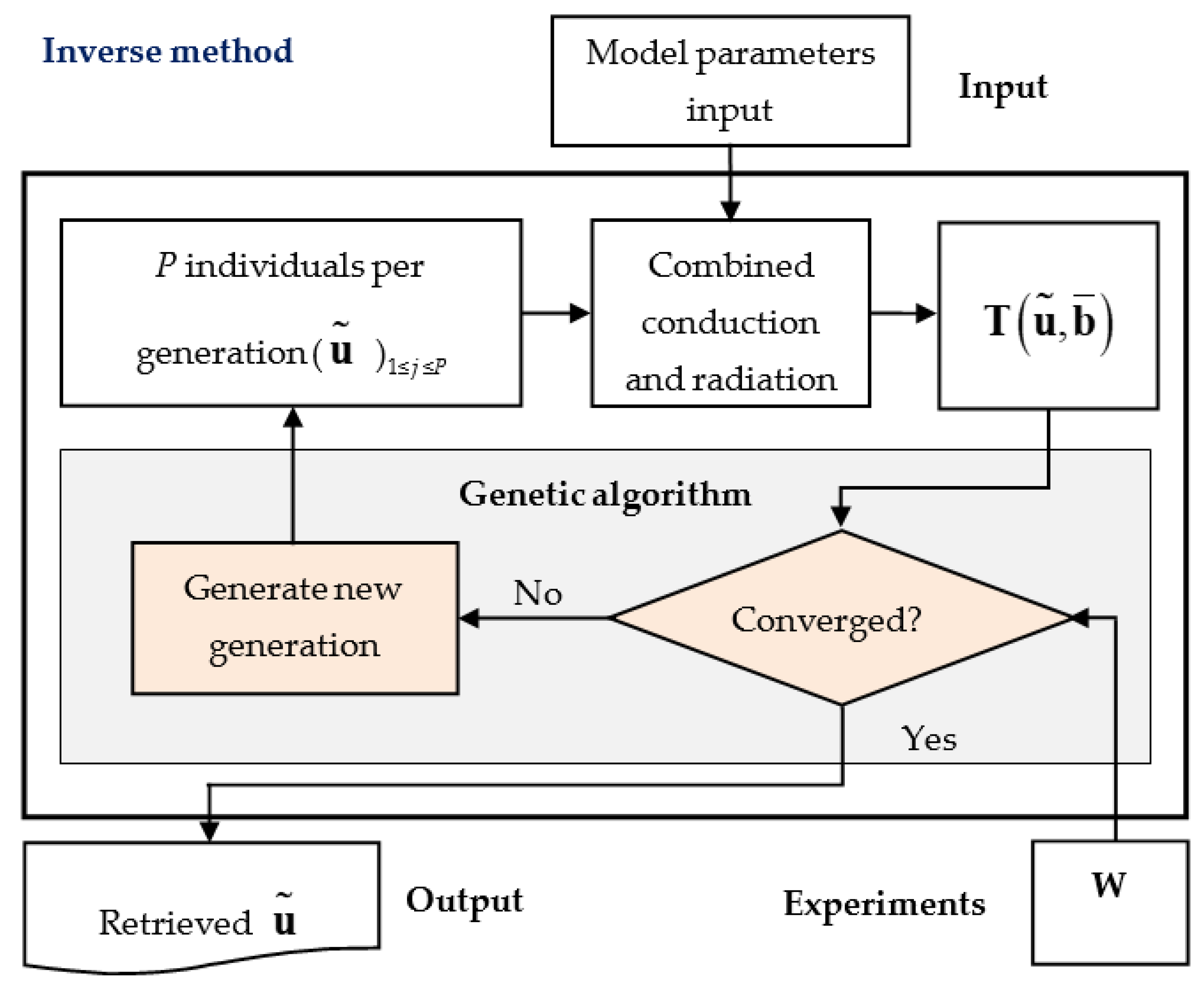
Transient coupled conductive and radiative heat transfer, in an absorbing and isotropic scattering gray solid slab with a thickness of L, were considered. The physical model of the slab, as well as the associated coordinate system, are shown in Figure 1. As the geometry considered was a solid slab, convection was not considered in the present study. In addition, the geometry can be three-dimensional but only one direction is relevant; thus, only 1-D combined conductive and radiative heat transfer was investigated. The boundaries of the slab were assumed to be diffuse and gray opaque, with an emissivity of ε₀ for x = 0, and ε_L for x = L, and the temperatures of the two walls were fixed at T_L and T_H, respectively. The extinction coefficient β, the scattering albedo ω, the thermal conductivity k_c, the density ρ, and the specific heat c_p of the slab were assumed to be constant in the present study.

The energy conservation equation for the slab can be written as [23,24]

$$\rho c_{\mathrm{p}}\frac{\partial T}{\partial t}=\frac{\partial }{\partial x}\left(k_{\mathrm{c}}\frac{\partial T\left(x,t\right)}{\partial x}\right)-\frac{\partial q_r^{″}\left(x,t\right)}{\partial x}$$

(1)

where T(x,t) denotes the temperature at position x and time t, and $q_r^{″}\left(x,t\right)$ is the radiative heat flux. The gradient of the radiative heat flux can be calculated from [23,24].

$$\frac{\partial q_r^{″}\left(x,t\right)}{\partial x}=4\pi n^2{I}_{\mathrm{b}}\left[T(x,t)\right]-G\left(x,t\right)$$

(2)

where $I_{\mathrm{b}}\left[T(x,t)\right]$ is the blackbody radiation intensity, and $G$ is the fluence rate defined as $G(\widehat{r})={\displaystyle \underset{4\pi }{\int }I(\widehat{s},\widehat{r})d\mathsf{\Omega }}$. The intensity $I(\widehat{s},\widehat{r})$ at location $\widehat{r}$ in direction $\widehat{s}$ is governed by the radiative transfer equation (RTE), written as [23,24]

$$\widehat{s}\cdot \nabla I=-\left(\kappa +{\sigma }_{\mathrm{s}}\right)I+\kappa n^2{I}_{\mathrm{b}}\left[T(\widehat{r},t)\right]+\frac{{\sigma }_{\mathrm{s}}}{4\pi }{\displaystyle {\int }_{4\pi }\mathsf{\Phi }\left({\widehat{s}}^{\prime },\widehat{s}\right)Id{\mathsf{\Omega }}^{\prime }}$$

(3)

where κ is the absorption coefficient and n is the refractive index, while ${\sigma }_{\mathrm{s}}$ and $\mathsf{\Phi }\left({\widehat{s}}^{\prime },\widehat{s}\right)$ are the scattering coefficient and phase function of scattering, respectively.

Corresponding to the physical model shown in Figure 1, the boundary and initial conditions can be written as

$$T\left(0,t\right)=T_{\mathrm{H}},T\left(L,t\right)=T_{\mathrm{L}}, \mathrm{and} T\left(x,0\right)=T_0$$

(4)

where T_H and T_L are the temperatures at the walls of x = 0 and x = L, respectively, while T₀ is the initial temperature. The transient temperature T(x_s, t) at sensor position x_s can be predicted by solving Equations (1)–(4).

2.2. Inverse Method

In order to maintain the generality of the method, we assumed that the unknown conductive and radiative properties to be retrieved were labeled as $u\in {ℝ}^{N_{\mathrm{P}}\times 1}$, where N_p is the number of unknown parameters. The model parameters were assumed to be $b\in {ℝ}^{N_{\mathrm{q}}\times 1}$, where N_q is the number of model parameters. The predicted transient temperature at location x_s was $T\left(\tilde{u},\overline{b}\right)\in {ℝ}^{N_{\mathrm{S}}\times N_{\mathrm{t}}}$, where $\tilde{u}$ is the retrieved value of u, and $\overline{b}$ is the measured value of parameter b, N_t is the number of sampling points, and N_S is the number of sensor positions. The transient temperature history measured in the ‘experiment’ was expressed as $W\in {ℝ}^{N_{\mathrm{S}}\times N_{\mathrm{t}}}$.

The inverse problem was defined as an optimization problem of finding the parameter vector u, for which the transient temperature history $T\left(\tilde{u},\overline{b}\right)$ at location x_s predicted from combined conduction and radiation was closest to the experimental data W; thus, the parameter vector u could be determined by minimizing an objective function defined as

$$F\left(u\right)=\Vert T\left(u,\overline{b}\right)-W\Vert$$

(5)

Thus,

$$\tilde{u}=\underset{u}{\arg \min }F\left(u\right)=\underset{u}{\arg \min }\Vert T\left(u,\overline{b}\right)-W\Vert$$

(6)

The genetic algorithm (GA), which is widely used for complex, ill-posed problems [25,26,27], was employed to solve the inverse identification problem. Figure 2 shows the block diagram of the GA-based inverse method used to determine parameter vector $\tilde{u}$.

2.3. Uncertainty Estimation and Design of Experiment

In the present study, a mathematical technique based on the stochastic Cramér–Rao lower bound (sCRB) is presented; the method aimed to take the measurement noise and the model parameter uncertainties of combined conduction and radiation into account for an a priori uncertainty estimation of the retrieved properties. Assuming that u* is the actual value of parameter vector u, the actual measurement W can be expressed as

$$W=T\left(u^{*},\overline{b}\right)+e_{\mathrm{tot}}$$

(7)

where $e_{\mathrm{tot}}\in {ℝ}^{N_{\mathrm{S}}\times N_{\mathrm{t}}}$ is the total error vector, and the total error vector at time t_k can be expressed as

$$e_{\mathrm{tot},k}=\left[W_k-T_k\left(u^{*},\overline{b}\right)\right]-E\left[W_k-T_k\left(u^{*},\overline{b}\right)\right], k=1,2,\dots ,N_{\mathrm{t}}$$

(8)

where $E\left[W_k-T_k\left(u^{*},\overline{b}\right)\right]$ is the expected value of quantity $\left[W_k-T_k\left(u^{*},\overline{b}\right)\right]$. The total error vector, $e_{\mathrm{tot}}$, contains two components, i.e., $e_{\mathrm{tot}}=e_{\exp }+e_{\mathrm{pred}}$, where $e_{\exp }$ and $e_{\mathrm{pred}}$ are the error vectors due to measurement noise and modeling uncertainties, respectively. The measurement error $e_{\exp }$ is composed of systematic and random components, as the state-of-the-art techniques and devices used for temperature measurement provide a rather low level of systematic error, and the reproducible nature of the systematic error makes it possible to estimate the bias on the measured data by means of a calibration procedure; this manuscript restricts discussions that the measurements contain only the random component of uncertainties, and the random error is assumed to be Gaussian while distributed with a mean of zero and a variance of ${\sigma }_{\exp ,k}^2$. The modeling error, $e_{\mathrm{pred}}$, can also be divided into two parts: the modeling error due to the use of inaccurate model parameter vector b, and the modeling error due to the use of inaccurate physical models (such as simplification of the physical models, or the use of inaccurate numerical methods). In this study, we assumed that the physical model was perfect; thus, the modeling error was affected only by the inaccurate model parameters.

The Cramér–Rao inequality theorem states that the covariance matrix of the deviation between the true and the estimated parameters is bounded from below by the inverse of the Fisher information matrix M [15,16,17]

$$E\left[\left(\tilde{u}-u^{*}\right){\left(\tilde{u}-u^{*}\right)}^{\mathrm{T}}\right]\ge M^{-1}$$

(9)

where, the Fisher information matrix can be calculated from

$$M=E\left\{\left[\frac{\partial }{\partial u}\ln L\left(W|u\right)\right] {\left[\frac{\partial }{\partial u}\ln L\left(W|u\right)\right]}^T\right\}$$

(10)

where M is a matrix with $N_{\mathrm{p}}\times N_{\mathrm{p}}$ dimensions, and $\ln L\left(W|u\right)$ is the log-likelihood of W given the parameter vector u; the likelihood of the data is normally distributed and is given by [15,16,17]

$$\begin{array}{l}L\left(W|u\right)={\left[{\left(2\pi \right)}^{N_{\mathrm{t}}{N}_{\mathrm{S}}}{\displaystyle \prod }_{k=1}^{N_{\mathrm{t}}}\mathrm{Det}\left(V_k\right)\right]}^{-1/2}\\ \times \exp \left\{{\displaystyle \sum _{k=1}^{N_{\mathrm{t}}}-\frac{1}{2}{\left[T_k\left(u^{*},\overline{b}\right)-W_k\right]}^{\mathrm{T}}{V}_k^{-1}\left[T_k\left(u^{*},\overline{b}\right)-W_k\right]}\right\}\end{array}$$

(11)

where $V_k$ is the total error variance, expressed as

$$V_k=E\left(e_{\mathrm{tot},k}{e}_{\mathrm{tot},k}^{\mathrm{T}}\right)$$

(12)

The total error includes contributions of both the measurement noise and the modeling error

$$V_k={\Theta }_{k}G{\Theta }_k^{\mathrm{T}}+S_k$$

(13)

where $S_k=E\left(e_{\exp ,k}{e}_{\exp ,k}^{\mathrm{T}}\right)=E\left\{\left[W_k-E\left(W_k\right)\right]{\left[W_k-E\left(W_k\right)\right]}^{\mathrm{T}}\right\}$ is the measurement variance, while ${\Theta }_{k}G{\Theta }_k^{\mathrm{T}}$ is the contribution of the uncertain model parameters, where $G\in {ℝ}^{N_{\mathrm{q}}\times N_{\mathrm{q}}}$ is the covariance matrix of the uncertain modal parameter vector b, and ${\Theta }_k$ is the sensitivity matrix of the temperature prediction $T$ with respect to the uncertain parameter vector b; this can be expressed as

$${\left({\Theta }_k\right)}_{i,q}=\frac{\partial T_i\left(t_k,u,b\right)}{\partial b_q}, i=1, 2, \dots , N_{\mathrm{S}}, q=1, 2, \dots , N_{\mathrm{q}}$$

(14)

Equation (11) can be rewritten as

$$\begin{array}{l}\ln L\left(W|u\right)=-\frac{1}{2}{N}_{\mathrm{t}}{N}_{\mathrm{S}}\ln \left(2\pi \right)-\frac{1}{2}{\displaystyle \sum _{k=1}^{N_{\mathrm{t}}}\ln \left[\mathrm{Det}\left(V_k\right)\right]}\\ -\frac{1}{2}{\displaystyle \sum _{k=1}^{N_{\mathrm{t}}}{\left[T_k\left(u^{*},\overline{b}\right)-W_k\right]}^{\mathrm{T}}{V}_k^{-1}\left[T_k\left(u^{*},\overline{b}\right)-W_k\right]}\end{array}$$

(15)

The first term of the right side is constant, thus

$$\begin{array}{l}\ln L\left(W|u\right)=\mathrm{const}-\frac{1}{2}{\displaystyle \sum _{k=1}^{N_{\mathrm{t}}}\ln \left[\mathrm{Det}\left(V_k\right)\right]}\\ -\frac{1}{2}{\displaystyle \sum _{k=1}^{N_{\mathrm{t}}}{\left[T_k\left(u^{*},\overline{b}\right)-W_k\right]}^{\mathrm{T}}{V}_k^{-1}\left[T_k\left(u^{*},\overline{b}\right)-W_k\right]}\end{array}$$

(16)

Therefore, the Fisher information matrix can be calculated from

$$\begin{array}{l}{\left(M\right)}_{lm}={\displaystyle \sum _{k=1}^{N_{\mathrm{t}}}\{{\left[\frac{\partial T_k\left(u^{*},\overline{b}\right)}{\partial u_m}\right]}^{\mathrm{T}}{V}_k^{-1}\left[\frac{\partial T_k\left(u^{*},\overline{b}\right)}{\partial u_l}\right]} \\ +\frac{1}{2}Tr\left[V_k^{-1}\frac{\partial V_k\left(u\right)}{\partial u_l}{V}_k^{-1}\frac{\partial V_k\left(u\right)}{\partial u_m}\right]\}, l,m=1,2,\dots ,N_{\mathrm{P}}\end{array}$$

(17)

The effect of the trace term is very small and can be neglected [17]; thus, the Fisher information matrix can be approximated by

$${\left(M\right)}_{lm}\approx {\displaystyle \sum _{k=1}^{N_{\mathrm{t}}}\left\{{\left[\frac{\partial T_k\left(u^{*},\overline{b}\right)}{\partial u_m}\right]}^{\mathrm{T}}{V}_k^{-1}\left[\frac{\partial T_k\left(u^{*},\overline{b}\right)}{\partial u_l}\right]\right\},} l,m=1,2,\dots ,N_{\mathrm{P}}$$

(18)

The lower bound for the variances of the parameters to be retrieved can be estimated as

$${\sigma }_{u_i,\mathrm{LB}}^2={\left(M^{-1}\right)}_{ii}, i=1, 2, \dots , N_{\mathrm{p}}$$

(19)

The ${\sigma }_{u_i,\mathrm{LB}}^2$ values could be used to qualitatively evaluate the retrieved results as well as the inverse identification models, and thus, could be employed in the method used to design the experiment. For inverse problems with only one parameter to be retrieved, the Fisher information matrix M can be reduced to a scalar M, ${\sigma }_{u,\mathrm{LB}}^2=1/M$.

The algorithm for determining the optimal sensor position for inverse conductive and radiative heat transfer is shown in Figure 3 as follows:

Step 1: Identify the mean value $\overline{b}$ of b and the corresponding covariance matrix G;

Step 2: Identify possible sensor positions, and chose an initial sensor position;

Step 3: Solve the forward problem, predict $T\left(u,\overline{b}\right)$ and the corresponding sensitivity $\Theta$, then estimate the experimental error ${\sigma }_{\exp }^2$;

Step 4: Estimate ${\sigma }_{u,\mathrm{LB}}^2$ for the retrieved parameter $\tilde{u}$;

Step 5: Update the sensor position and go to step 3, then estimate ${\sigma }_{u,\mathrm{LB}}^2$ for all sensor positions;

Step 6: Evaluate the different sensor positions and find the optimal sensor position.

3. Results and Discussion

We ‘simulated’ the measurements by using the output of the forward model with the actual values of the unknown parameters to be retrieved, and the measurements were corrupted by Gaussian noise with a mean and standard deviation of zero. In this way, we were able to perform numerical experiments to illustrate the uncertainty of the method of analysis, and to show the designed optimal sensor position.

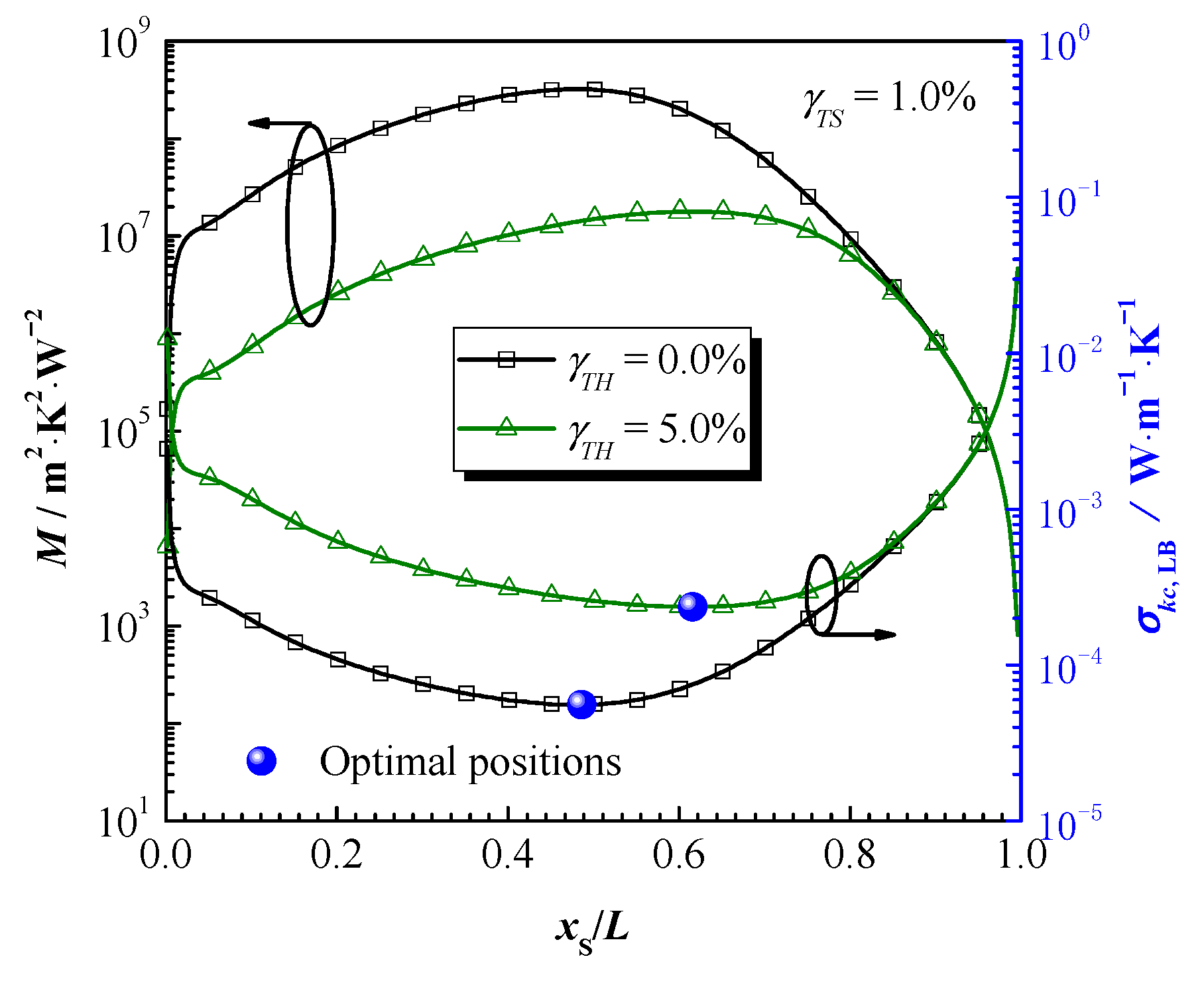
3.1. Identification of Conductive Thermal Conductivity: The Optimal Experimental Design

For the first example, we considered an absorbing and isotropic scattering gray slab, as shown in Figure 1. The slab had volumetric heat capacity c_v = 4×10⁵ J/(m³∙K), refractive index n = 1.0, extinction coefficient β = 2000 m⁻¹, and scattering albedo ω = 0.8; furthermore, the thickness of the slab was L = 0.02 m, and the boundary emissivities for x = 0 and for x = L were ε₀ = ε_L = 0.8. The initial temperature of the slab was T₀ = 300 K; the temperature of the two slab walls were fixed at T_H = 1000 K for x = 0, and T_L = 300 K for x = L, respectively. The conductive thermal conductivity k_c was assumed to be unknown and needed to be retrieved, and the actual value of k_c was 0.02 W/(m∙K). The ‘measured temperature’ was simulated by adding Gaussian noise to the solution of combined conduction and radiation, and various noise levels, ${\gamma }_{T\mathrm{S}}\%$, were considered in the present study. The standard deviation, ${\sigma }_{\exp ,k}$, of the ‘measured temperature’, at time t_k, could be calculated from

$${\sigma }_{\exp ,k}={\gamma }_{T\mathrm{S}}\% \cdot T\left(x_{\mathrm{S}},t_k\right)\cdot \xi$$

(20)

where $\xi$ is a normal distribution number with a mean of zero and a standard deviation of unity. We also considered that the boundary temperature T_H at x = L was not accurate, and its value was distributed about the mean value of T_H = 1000 K with a normally distributed noise ${\gamma }_{TH}\%$; similarly, the standard deviation ${\sigma }_{TH}$ of T_H could be calculated from ${\sigma }_{TH}={\gamma }_{TH}\% \cdot T_{\mathrm{H}}\cdot \xi$. Here, the considered time duration of the ‘experiment’ was t_S = 200 s, and the sampling increment of time was Δt = 2 s.

Figure 4 shows the estimated lower bound, ${\sigma }_{k_c,\mathrm{LB}}$, for the standard deviation of the conductive thermal conductivity, k_c, with respect to various measurement noise ${\gamma }_{T\mathrm{S}}\%$ and boundary temperature error ${\gamma }_{TH}\%$ values; the values considered for ${\gamma }_{T\mathrm{S}}\%$ and ${\gamma }_{TH}\%$ ranged from 1% to 9%, with an increment of 2%, and the temperature sensor was located at x_s = L/2.

First, it was obvious that the ${\sigma }_{k_c,\mathrm{LB}}$ values increased with the increasing measurement noise ${\gamma }_{T\mathrm{S}}\%$, as well as the increasing ${\gamma }_{TH}\%$ values, which indicated that the accuracy of the retrieved parameters could be improved by performing an accurate experiment, and by using accurate model parameters. It is also interesting to note that the ${\sigma }_{k_c,\mathrm{LB}}$ value for ${\gamma }_{T\mathrm{S}}\%$ = 3% and ${\gamma }_{TH}\%$ = 1% was smaller than that for ${\gamma }_{T\mathrm{S}}\%$ = 1% and ${\gamma }_{TH}\%$ = 9%; the decrease in measurement noise ${\gamma }_{T\mathrm{S}}\%$ (from 3% to 1%) did not result in a lower value of ${\sigma }_{k_c,\mathrm{LB}}$. This indicated that the accuracy of the retrieved parameter was affected comprehensively by the measurement noise and the model parameter uncertainty, and neither of the two factors could be neglected. Therefore, for some inverse identification problems, only trying to perform accurate experiments may not be sufficient in terms of improving the accuracy of the retrieved parameters.

Figure 5 presents the estimated Fisher information matrix M (M is reduced to a scalar M as M has only one element), and the lower bound ${\sigma }_{k_c,\mathrm{LB}}$, for the standard deviation of the conductive thermal conductivity k_c as a function of the dimensionless sensor position x_s/L. The measurement noise was assumed to be ${\gamma }_{T\mathrm{S}}\%$ = 1%, and two different boundary temperature noise values, ${\gamma }_{TH}\%$ = 0% and ${\gamma }_{TH}\%$ = 5%, were investigated separately.

It can be seen from Figure 5 that the ${\sigma }_{k_c,\mathrm{LB}}$ values first decreased, and then presented an increasing tendency with the increasing of the dimensionless sensor position x_s/L. For ${\gamma }_{TH}\%$ = 0%, the optimal sensor position was in the vicinity of x_s/L = 0.5, and the minimum value of ${\sigma }_{k_c,\mathrm{LB}}$ was about $5.5\times {10}^{-5}$ W/(m∙K). Compared with the results for ${\gamma }_{TH}\%$ = 0%, the minimum value of ${\sigma }_{k_c,\mathrm{LB}}$ for ${\gamma }_{TH}\%$ = 5% was increased to about $2.4\times {10}^{-4}$ W/(m∙K); furthermore, the optimal sensor position moved from x_s/L = 0.5 to a position in the vicinity of x_s/L = 0.6, due to the fact that the boundary temperature error ${\gamma }_{TH}\%$ affected the solution of the forward problem, especially for positions that were close to the boundary x = 0. Therefore, the sensor should be placed far away from the boundary to reduce its error effect.

The time-consuming Monte Carlo (MC) technique was employed to validate the designed sensor positions. We assumed that the three potential positions, x_s/L = 0.5, 0.6, and 0.9, were available to place the temperature sensor for both ${\gamma }_{TH}\%$ = 0% and ${\gamma }_{TH}\%$ = 5%, respectively. For each sensor position and boundary temperature error ${\gamma }_{TH}\%$, 1000 independent inverse identifications were performed to retrieve k_c; thus, the standard deviations of the retrieved k_c were calculated and compared with the ${\sigma }_{k_c,\mathrm{LB}}$ value estimated via the CRB-based error analysis method. The results are presented in

Table 1. Comparison of standard deviation of the retrieved conductive thermal conductivity estimated from the CRB method and MC simulations for various boundary temperature error values of ${\gamma }_{TH}\%$ = 0% and 0.5, and various dimensionless sensor positions of x_s/L = 0.5, 0.6 and 0.9, respectively.

Sensor Position	Standard Deviation of Thermal Conductivity, W/(m∙K)
	${\mathit{\gamma }}_{\mathit{T}\mathit{H}}\%$ = 0% and ${\mathit{\gamma }}_{\mathit{T}\mathit{S}}\%$ = 1%		${\mathit{\gamma }}_{\mathit{T}\mathit{H}}\% =5\% \mathbf{and} {\mathit{\gamma }}_{\mathit{T}\mathit{S}}\%=1\%$
	CRB	MC	CRB	MC
xs/L = 0.5	0.55 × 10−4	1.0 × 10−4	2.6 × 10−4	5.2 × 10−4
xs/L = 0.6	0.70 × 10−4	1.3 × 10−4	2.4 × 10−4	4.1 × 10−4
xs/L = 0.9	11.1 × 10−4	18.7 × 10−4	11.2 × 10−4	19.3 × 10−4

.

It can be seen that a large discrepancy between the values estimated from the two methods was observed. This was due to the fact that the CRB-based method gave the lower bound of the uncertainty of the retrieved k_c; however, the aim of the present study was not to prove the correct quantitative error values. According to the MC simulation results, the best sensor position was x_s/L = 0.5 and x_s/L = 0.6 for ${\gamma }_{TH}\%$ = 0% and ${\gamma }_{TH}\%$ = 5%, respectively, while the worst position was x_s/L = 0.9 for both ${\gamma }_{TH}\%$ = 0% and ${\gamma }_{TH}\%$ = 5%; this is consistent with the positions estimated using the CRB method. It indicates that the CRB method can be used to estimate the optimal experimental design for identification problems related to thermal properties.

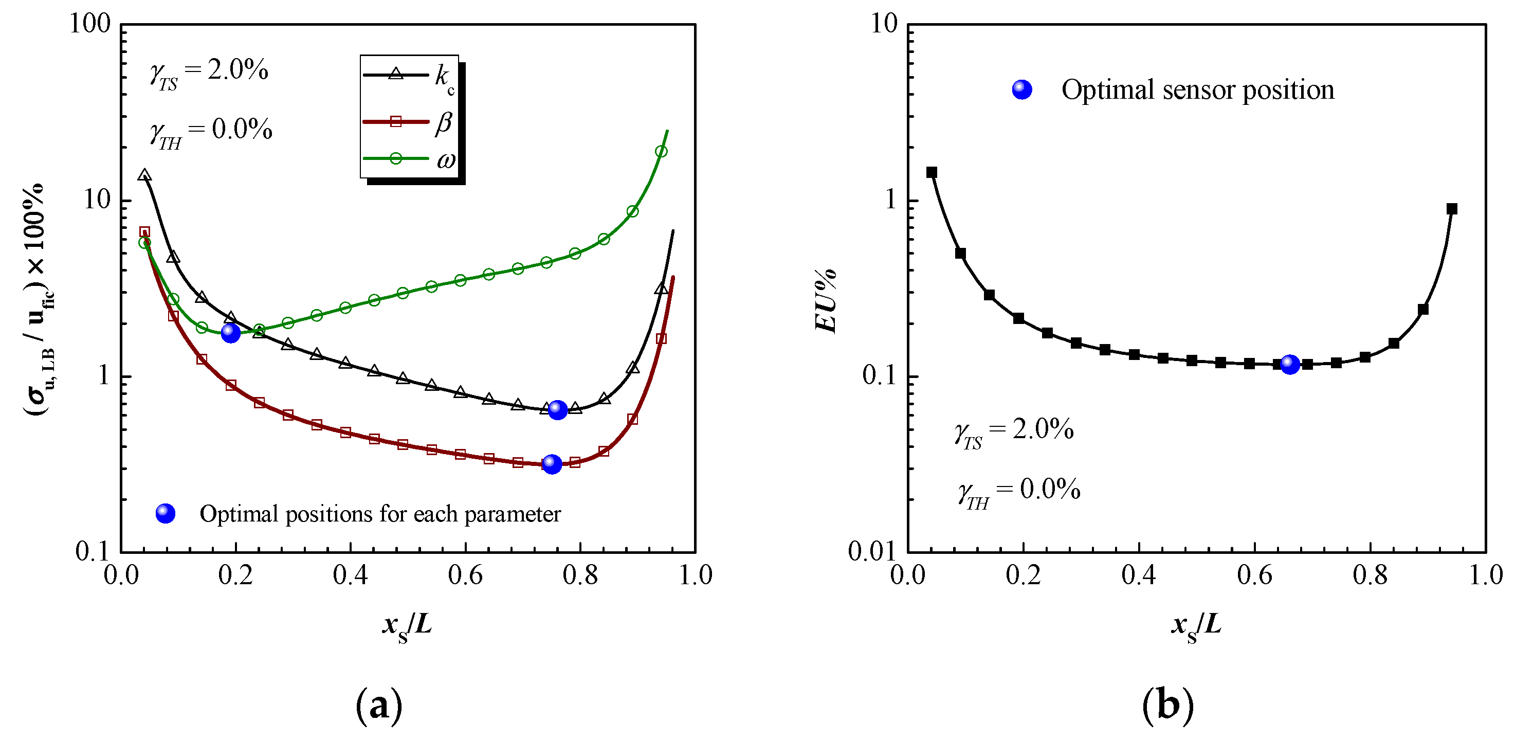
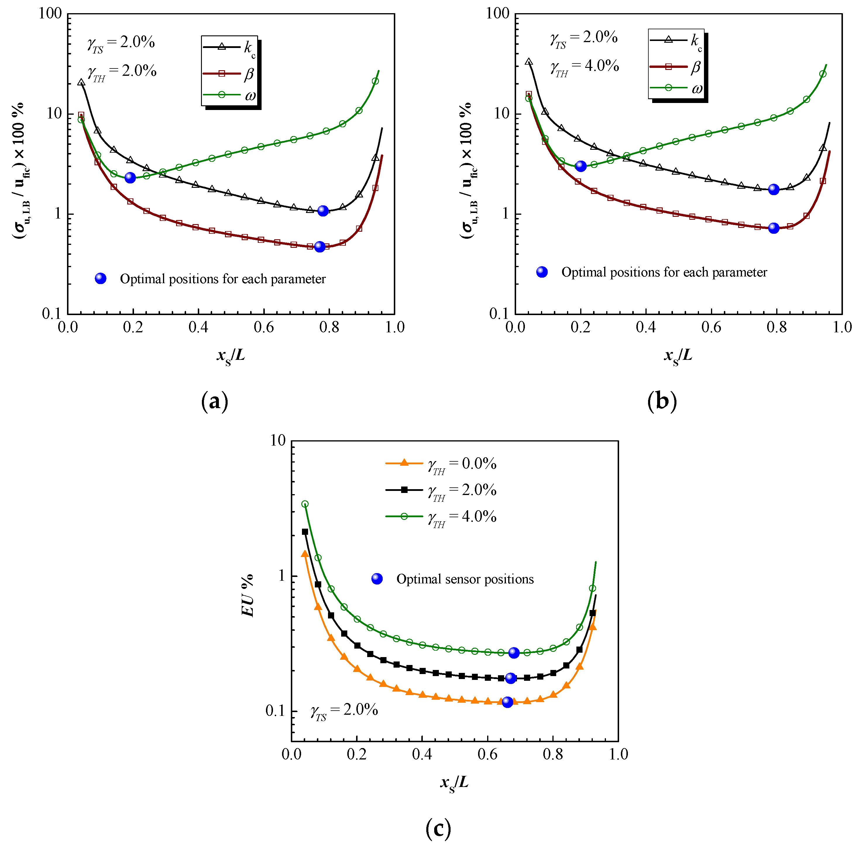
3.2. Identification of Conductive and Radiative Properties: The Optimal Experimental Design

For problems regarding identification of conductive and radiative multiple properties, we considered the same physical model that was discussed in Section 3.1. The conductive thermal conductivity k_c, extinction coefficient β, and scattering albedo ω of the slab were assumed to be unknown, and thus, needed to be retrieved, and their actual values were such that k_c = 0.02 W/(m∙K), β = 2000 m⁻¹, and ω = 0.8, respectively. The time duration of the ‘experiment’ was t_S = 1000 s, and the sampling increment of time was Δt = 2 s. The other parameters including the geometry parameter, the boundary condition parameters, and other properties were the same as those presented in Section 3.1.

For optimal experimental design problems involving the retrieving of only one parameter, the optimal sensor position could be easily identified according to the lower bound for the standard deviation values of the parameter to be retrieved. The optimal sensor position for multiple-parameter identification problems could not be determined directly from the lower bound for the standard deviation ${\sigma }_{u_i,\mathrm{LB}}^2$ of the parameter to be retrieved, as the minimum ${\sigma }_{u_i,\mathrm{LB}}^2$ for each parameter would not necessarily lead to the same sensor location. For this reason, it was necessary to define a new parameter to evaluate the retrieved parameters; in the present study, the parameter EU% was defined

$$EU\%={\displaystyle \sum _{i=1}^{N_{\mathrm{p}}}\left|\frac{\sqrt{\frac{1}{N_{\mathrm{t}}}{\displaystyle \sum _{k=1}^{N_{\mathrm{t}}}{\left[T_{\mathrm{S},\mathrm{pred}}\left(u_{i,\mathrm{fic}}+{\sigma }_{u_i,\mathrm{LB}},x_{\mathrm{e}}, t_k\right)\right]}^2}}}{\sqrt{\frac{1}{N_{\mathrm{t}}}{\displaystyle \sum _{k=1}^{N_{\mathrm{t}}}{\left[T_{\mathrm{S},\mathrm{pred}}\left(u_{i,\mathrm{fic}},x_{\mathrm{e}}, t_k\right)\right]}^2}}}-1\right|\times 100\%}$$

(21)

where $N_{\mathrm{t}}$ is the number of sampling points, $T_{\mathrm{S},\mathrm{pred}}\left(u_{i,\mathrm{fic}},x_{\mathrm{e}}, t_k\right)$ is the predicted temperature at time t_k and location x_e using the fictitious parameter value $u_{i,\mathrm{fic}}$, and in the present study, we assumed that x_e = L/2. The parameter EU% measured the integrated uncertainty of the recovered transient temperature response; the lower the EU%, the better the retrieved parameters. Thus, the best sensor position was the one that featured the lowest EU%.

Figure 6 presents the estimated EU% with respect to various measurement noise ${\gamma }_{T\mathrm{S}}\%$ and boundary temperature error ${\gamma }_{TH}\%$ values. The values considered for ${\gamma }_{T\mathrm{S}}\%$ and ${\gamma }_{TH}\%$ ranged from 1 to 5%, with an increment of 1%. The temperature sensor was located at x_s/L = 0.5. As with those used for one-parameter identification problems, the accuracy of the retrieved parameters could have been improved by performing more accurate experiments, and by using accurate model parameters when solving inverse conductive and radiative heat transfer problems.

Figure 7a presents the values of ${\sigma }_{u,\mathrm{LB}}/u_{\mathrm{fic}}$ with respect to dimensionless sensor location x_s/L; the measurement noise considered here was ${\gamma }_{TS}\%$ = 2.0%. It is obvious that smaller ${\sigma }_{u,\mathrm{LB}}/u_{\mathrm{fic}}$ values led to better retrieved results. The dimensionless positions corresponding to the minimum value of ${\sigma }_{u,\mathrm{LB}}/u_{\mathrm{fic}}$ for k_c, β and ω were x_s/L = 0.76, 0.75, and 0.19, respectively, and the positions should have been the optimal sensor position for each parameter. It is interesting to note that the positions for each parameter were not consistent; therefore, the overall optimal sensor position could not be directly determined.

Figure 7b shows the EU% values with respect to the dimensionless sensor location x_s/L; the position corresponding to the minimum value of EU% was x_s/L = 0.66, and the position should have been the optimal sensor position for the multiple-property identification problem. In fact, as the variation of x_s/L between 0.4 and 0.8 led to only slight changes in the EU% values, the temperature sensor could have been placed at any position within this range. Therefore, the main consideration for researchers or engineers should be the ease and reliability of sensor installation.

Figure 8a,b show the values of ${\sigma }_{u,\mathrm{LB}}/u_{\mathrm{fic}}$ with respect to the dimensionless sensor position x_s/L for the measurement noise value of ${\gamma }_{TS}\%$ = 2.0%, and the boundary temperature error of ${\gamma }_{TH}\%$ = 2.0% and ${\gamma }_{TH}\%$ = 4.0%, respectively. Compared with the results reported in Figure 7a, the ${\sigma }_{u,\mathrm{LB}}/u_{\mathrm{fic}}$ increased with the increasing of the ${\gamma }_{TH}\%$ values. The optimal sensor positions for k_c, β and ω moved slightly further away from the boundary x = 0 as ${\gamma }_{TH}\%$ increased. Figure 8c reports the EU% as a function of the dimensionless sensor location for various ${\gamma }_{TH}\%$ values of 0.0%, 2.0%, and 4.0%, respectively. It is obvious that the EU% values increased dramatically with the increasing of ${\gamma }_{TH}\%$, which means that the uncertainty of the boundary temperature had an obvious effect on the retrieved results. Furthermore, the optimal sensor position displayed a tendency to move slightly further away from the boundary x = 0. As the EU% values corresponding to x_s/L between 0.4 and 0.8 changed slightly within this range, the temperature sensor could have been placed at any position within the range.

As only one sensor position was designed, the total error variance $V_k$ and the experimental error variance $S_k$, shown in Equation (13), were reduced to scalar V_k and S_k; thus, if O_k = V_k − S_k, the quantity O_k could then be used to measure the error variance caused by an inaccurate boundary temperature T_H. Therefore, the S_k/V_k and O_k/V_k values could be used to measure the relative contribution of the experimental noise and boundary temperature error to the total error at time t_k, and thus, the integrated error contribution of experimental noise and boundary temperature T_H over the whole time duration could be expressed as

$${{\rm E}}_{\mathrm{f}}\left(W_k\right)={\displaystyle \sum _{k=1}^{N_{\mathrm{t}}}{S}_k}/{\displaystyle \sum _{k=1}^{N_{\mathrm{t}}}{V}_k}, {{\rm E}}_{\mathrm{f}}\left(T_{\mathrm{H}}\right)={\displaystyle \sum _{k=1}^{N_{\mathrm{t}}}{O}_k\left(T_{\mathrm{H}}\right)}/{\displaystyle \sum _{k=1}^{N_{\mathrm{t}}}{V}_k}$$

(22)

Figure 9a presents S_k/V_k and O_k/V_k as a function of time t. At this point, the measurement noise was still ${\gamma }_{TS}\%$ = 2.0%, and the boundary temperature error considered in the present study was such that ${\gamma }_{TH}\%$ = 2.0% and ${\gamma }_{TH}\%$ = 4.0%, respectively. The value of ${\gamma }_{TH}\%$ affected the contribution of the boundary temperature uncertainty to the overall error, and the O_k/V_k values for ${\gamma }_{TH}\%$ = 2.0% were always smaller than those for ${\gamma }_{TH}\%$ = 4.0%. The S_k/V_k and O_k/V_k values varied with time; first, the experimental error predominated, but, as time went on, the contribution of the boundary temperature error gradually increased, and started to become predominant, indicating that the main contribution factors changed in an alternating manner during the entirety of the time duration.

Figure 9b shows the integrated error contribution of the two error resources. First, it can be seen that the boundary error contribution was predominant for both ${\gamma }_{TH}\%$ = 2.0% and ${\gamma }_{TH}\%$ = 4.0%, and the error contribution was about 67% and 88%, respectively. Therefore, in order to improve the accuracy of the retrieved conductive and radiative properties, an effective method would involve trying to improve the accuracy of the boundary temperature, T_H, rather than concentrating on transient temperature measurements.

4. Conclusions

In the present work, we proposed a stochastic Cramér–Rao bound (sCRB)-based numerical methodology to estimate the error of the conductive and radiative properties of participating medium that was recovered from transient temperature measurements by solving inverse heat transfer problems. The measurement noise and the inaccurate model parameters were both taken into account in the analysis. The inverse identification problems of retrieving only one parameter and retrieving multiple parameters were illustrated separately. The proposed sCRB-based method was numerically validated by the time-consuming Monte Carlo simulations, and it was shown that the method was able to determine, a priori, the error of the retrieved parameters. Based on the method, the optimal temperature sensor positions were designed to improve the accuracy of the retrieved parameters, and the relative error contributions of the error sources were also estimated.

The results show that: (1) the optimal sensor position is comprehensively determined by the factors of measurement noise as well as the uncertainties of inaccurate model parameters, and the optimal position varies with the levels of the error sources; (2) for problems regarding multiple parameter identification, the optimal position for each parameter may not be consistent, and thus, the optimal sensor position for the identification problem should be evaluated by the comprehensive parameter EU%, which is defined in Equation (21); and (3) the relative error contributions for each error source vary according to their error level, and the estimated relative error contributions can provide suggestions for improving the accuracy of the retrieved parameters.

References

1. Coquard, R.; Rochais, D.; Baillis, D. Experimental investigations of the coupled conductive and radiative heat transfer in metallic/ceramic foams. Int. J. Heat Mass Transf. 2009, 52, 4907–4918. [Google Scholar] [CrossRef]
2. Das, R.; Mishra, S.C.; Uppaluri, R. Inverse analysis applied to retrieval of parameters and reconstruction of temperature field in a transient conduction-radiation heat transfer problem involving mixed boundary conditions. Int. Commun. Heat Mass Transf. 2010, 37, 52–57. [Google Scholar] [CrossRef]
3. Li, H.Y. Estimation of thermal properties in combined conduction and radiation. Int. J. Heat Mass Transf. 1999, 42, 565–572. [Google Scholar] [CrossRef]
4. Zmywaczyk, J.; Koniorczyk, P. Numerical solution of inverse radiative-conductive transient heat transfer problem in a grey participating medium. Int. J. Thermophys. 2009, 30, 1438–1451. [Google Scholar] [CrossRef]
5. Qi, H.; Niu, C.Y.; Gong, S.; Ren, Y.T.; Ruan, L.M. Application of the hybrid particle swarm optimization algorithms for simultaneous estimation of multi-parameters in a transient conduction-radiation problem. Int. J. Heat Mass Transf. 2015, 83, 428–440. [Google Scholar] [CrossRef]
6. Braiek, A.; Adili, A.; Albouchi, F.; Karkri, M.; Nasrallah, S.B. Estimation of radiative and conductive properties of a semitransparent medium using genetic algorithms. Meas. Sci. Technol. 2016, 27, 65601. [Google Scholar] [CrossRef]
7. Liu, Y.; Billaud, Y.; Saury, D.; Lemonnier, D. Simultaneous identification of thermal conductivity and absorption coefficient of a homogeneous medium. Int. Heat Transf. Conf. 2018, 8834–8841. [Google Scholar] [CrossRef]
8. Lazard, M.; Andre, S.; Maillet, D.; Baillis, D.; Degiovanni, A. Flash experiment on a semitransparent material: Interest of a reduced model. Inverse Probl. Eng. 2001, 9, 413–429. [Google Scholar] [CrossRef] [Green Version]
9. Zhao, S.Y.; Zhang, B.M.; Du, S.Y.; He, X.D. Inverse identification of thermal properties of fibrous insulation from transient temperature measurements. Int. J. Thermophys. 2009, 30, 2021–2035. [Google Scholar] [CrossRef]
10. Zhao, S.; Sun, X.; Li, Z.; Xie, W.; Meng, S.; Wang, C.; Zhang, W. Simultaneous retrieval of high temperature thermal conductivities, anisotropic radiative properties, and thermal contact resistance for ceramic foams. Appl. Therm. Eng. 2019, 146, 569–576. [Google Scholar] [CrossRef]
11. Sun, K.K.; Jung, B.S.; Kim, H.J.; Lee, W.I. Inverse estimation of thermophysical properties for anisotropic composite. Exp. Therm. Fluid Sci. 2003, 27, 697–704. [Google Scholar]
12. Sawaf, B.; Ozisik, M.N.; Jarny, Y. An inverse analysis to estimate linearly temperature dependent thermal conductivity components and heat capacity of an orthotropic medium. Int. J. Heat Mass Transf. 1995, 38, 3005–3010. [Google Scholar] [CrossRef]
13. Neto, A.J.S.; Özişik, M.N. An inverse problem of simultaneous estimation of radiation phase function, albedo and optical thickness. J. Quant. Spectrosc. Radiat. Transf. 1995, 53, 397–409. [Google Scholar] [CrossRef]
14. Lazard, M.; André, S.; Maillet, D.; Degiovanni, A. Radiative and conductive heat transfer: A coupled model for parameter estimation. High Temp.-High Press. 2000, 32, 9–17. [Google Scholar] [CrossRef]
15. Fadale, T.D.; Nenarokomov, A.V.; Emery, A.F. Uncertainties in parameter estimation: The inverse problem. Int. J. Heat Mass Transf. 1995, 38, 511–518. [Google Scholar] [CrossRef]
16. Fadale, T.D.; Nenarokomov, A.V.; Emery, A.F. Two approaches to optimal sensor locations. J. Heat Transf. 1995, 117, 373–379. [Google Scholar] [CrossRef]
17. Emery, A.F.; Nenarokomov, A.V.; Fadale, T.D. Uncertainties in parameter Estimation: The optimal experiment design. Int. J. Heat Mass Transf. 2000, 43, 3331–3339. [Google Scholar] [CrossRef]
18. Skog, I.; Nilsson, J.O.; Händel, P.; Nehorai, A. Inertial sensor arrays, Maximum Likelihood, and Cramér-Rao bound. IEEE Trans. Signal Process. 2016, 64, 4218–4227. [Google Scholar] [CrossRef] [Green Version]
19. Radich, B.M.; Buckley, K.M. EEG dipole localization bounds and MAP algorithms for head models with parameter uncertainties. IEEE Trans. BioMed. Eng. 1995, 42, 233–241. [Google Scholar] [CrossRef]
20. Abdallh, A.A.; Crevecoeur, G.; Dupré, L. Optimal needle placement for the accurate magnetic material quantification based on uncertainty analysis in the inverse approach. Meas. Sci. Technol. 2010, 21, 115703. [Google Scholar] [CrossRef]
21. Abdallh, A.A.; Crevecoeur, G.; Dupré, L. A priori experimental design for inverse identification of magnetic material properties of an electromagnetic device using uncertainty analysis. Compel-Int. J. Comput. Math. Electr. Electron. Eng. 2012, 31, 972–984. [Google Scholar] [CrossRef] [Green Version]
22. Abdallh, A.A.; Crevecoeur, G.; Dupré, L. Selection of measurement modality for magnetic material characterization of an electromagnetic device using stochastic uncertainty analysis. IEEE Trans. Magn. 2011, 47, 4564–4573. [Google Scholar] [CrossRef]
23. Modest, M.F. Radiative Heat Transfer; Academic Press: San Diego, CA, USA, 2003. [Google Scholar]
24. Howell, J.R.; Siegel, R.; Mengüç, M.P. Thermal Radiation Heat Transfer; Taylor and Francis: New York, NY, USA, 2011. [Google Scholar]
25. Czél, B.; Gróf, G. Genetic algorithm-based method for determination of temperature-dependent thermophysical properties. Int. J. Thermophys. 2009, 30, 1975–1991. [Google Scholar] [CrossRef]
26. Czél, B.; Gróf, G. Inverse identification of temperature-dependent thermal conductivity via genetic algorithm with cost function-based rearrangement of genes. Int. J. Heat Mass Transf. 2012, 55, 4254–4263. [Google Scholar] [CrossRef]
27. Czél, B.; Gróf, G. Simultaneous identification of temperature-dependent thermal properties via enhanced genetic algorithm. Int. J. Thermophys. 2012, 33, 1023–1041. [Google Scholar] [CrossRef]
Figure 1. Schematic of coupled conductive and radiative heat transfer in an absorbing and scattering slab.
Energies 14 06593 g001
Figure 2. Block diagram of the inverse method.
Energies 14 06593 g002
Figure 3. Flow chart of the optimal design of experiments based on the a priori estimation of the variance of the parameters to be retrieved.
Energies 14 06593 g003
Figure 4. The σ k c , LB values with respect to various ‘measured temperature’ error γ T S %   and various boundary temperature error γ T H %   values.
Energies 14 06593 g004
Figure 5. The values of M and σ k c , LB of conductive thermal conductivity to be retrieved as a function of the dimensionless sensor position xs/L.
Energies 14 06593 g005
Figure 6. The EU% values based on the CRB method at various errors of γ T H % and γ T S % .
Energies 14 06593 g006
Figure 7. The values of (a) σ u , LB / u fic and (b) EU% as a function of the dimensionless sensor location for γ T S % = 2.0% and γ T H % = 0.0%.
Energies 14 06593 g007
Figure 8. (a) The values of σ u , LB / u fic corresponding to γ T H % = 2.0%, (b) the values of σ u , LB / u fic corresponding to γ T H % = 4.0%, and (c) the EU% as a function of the dimensionless sensor location for various γ T H % values.
Energies 14 06593 g008
Figure 9. (a) The values of Sk/Vk and Ok/Vk with respect to different γ T H % values, and (b) the error contributions of TS,exp(t) and TH.
Energies 14 06593 g009