Numerical Simulation of Gas-Solid Two-Phase Erosion for Elbow and Tee Pipe in Gas Field

Abstract

Erosion caused by solid particles in a pipeline is one of the main problems endangering the safety production of the oil and gas industry, which may lead the equipment to malfunction or even fail. However, most of the previous studies focused on the standard elbow, and the erosion law of right-angle elbow and blind tee is rarely reported in the literature. This work aims to investigate the erosion law of different pipeline structures including 90° elbow, right-angle pipe, and tee pipe based on the production characteristics and engineering parameters of the gas field. An integrated CFD-DPM method is established including a realizable k-ε turbulence model, discrete phase model, and erosion rate prediction model. The accuracy of the model is evaluated by a series of experimental data of flow conditions of our previous work. Further, the erosion rate, pressure distributions, and particle trajectories in 90° elbow, right-angle pipe, and tee pipe under different flow velocities, particle mass flow rate, pipe diameter are investigated by applying the presented model. The results show that the blind tee has the most obvious growth rate, and the most serious erosion is located in the blind end of the pipe wall. The maximum erosion rate of the 1.5D is greater than that of the 3D elbow as a whole, and the 1.5D elbow is more concentrated in the serious erosion area. Furthermore, the erosion rate of the bend weld is much greater than that of the straight pipe weld. This study can provide a basis for the selection of different structural pipe fittings, thereby reducing the pipeline erosion rate and improving the integrity of the management of gas pipelines.

1. Introduction

Shale gas is a kind of unconventional natural gas existing in shale and mainly composed of methane, regarding as a clean and efficient energy resource [1]. In the process of shale gas exploitation, there are many challenges, one of which is the erosion of sand and gravel [2,3]. Although some filtering measures are taken to filter out solid particles in the produced gas during shale gas exploitation, it still cannot completely prevent the passage of some small particles [4]. In the shale gas gathering and transportation pipeline, the produced gas is driven by the energy of the reservoir, and the gas flow rate is fast [5]. The solid particles are carried by high-speed flowing gas and continuously impact the pipe wall, causing pipeline erosion, especially in the position where the flow direction changes, such as elbows, tees, etc. [6,7].

The erosion of solid particles in single-phase or multiphase flow is a very complex process. There are many factors that affect erosion, including fluid properties, particle properties (particle shape, particle size, particle material), particle impact speed and impact angle, etc. [4,8,9]. It is a great challenge to accurately predict the erosion of particles on the pipe wall. With the rise of computers and ever-growing computational power, the field of Computational Fluid Dynamics (CFD) became a commonly applied tool for generating solutions for fluid flows with or without solid interaction [10]. CFD is the process of mathematically modeling a physical phenomenon involving fluid flow and solving it numerically using computational prowess [11]. CFD has shown reliable performance in solving real-life problems, and it has been widely used in industrial applications. Therefore, CFD methods have gradually become one of the important methods for studying flow problems [12].

Many scholars have studied the erosion in the pipeline system under different operating conditions based on the CFD method with the help of computers [13,14,15]. The main advantage of CFD-based erosion analysis is that different factors affecting corrosion can be studied separately or in proper combination to find out the area where is more likely to suffer serious material loss. In addition, CFD-based erosion analysis can even predict the maximum erosion rate in the geometric structure that is difficult to analyze erosion by setting up an experimental device. Peng et al. [16] simulated elbow erosion of water pipe, including using a standard k-ε turbulent model for liquid flow, the DPM model for particle movement, and the E/CRC erosion model with particle-wall rebound model for particle erosion. The results show that the erosion rate increases with the increase of the flow rate, mass flow rate, and bending angle, and decreases with the increase of the diameter of the pipe or R/D. With the increase of particle size, the erosion rate decreases first and then increases, and there is a minimum when the particle size is 150 μm. Ejeh et al. [17] used Reynolds averaging navigator–stocks (RAS) and particle tracking modeling (PTM) to simulate fluid flow and track particle trajectory for crude pipeline 45°, 90°, 135°, and 180° elbows. The results show that the erosion rate is relatively higher at the elbows, and the serious degree of erosion area changes with the curvature of the pipe. In addition, the erosion rate is affected by the velocity, mass, and density of particles. The higher the particle velocity, mass, and density, the higher the erosion rate predicted. Laín et al. [18] used the Euler Lagrange method and Oka erosion model to study erosion of 90° elbows of the gas pipeline under the different factors. The results show that the increase of wall roughness significantly reduces the erosion rate, and the particles larger than the average particle size lead to a higher erosion rate. Moreover, the erosion rate decreases with the increase of particle mass flow rate. Parsi et al. [19] studied sand and gravel erosion in gas-dominant multiphase flow. They used three different apparent gas velocities, which were 10.1, 18.3, and 27.1 m/s, respectively, while the apparent velocity of liquid remained constant at 0.3 m/s. The sizes of sand and gravel used were 150 μm and 300 μm. Ogunsesan et al. [20] simulated the air-water multiphase flow and particle erosion behavior in a 76.2 mm diameter pipe. The minimum and maximum superficial velocity of the gas phase were 0.07 m/s and 40 m/s respectively, and the constant apparent velocity of the liquid phase was 0.3 m/s. The erosion under different flow patterns was considered. In our previous work [3], an integrated CFD-DPM model was established to investigate the erosion of the 90° elbow in a shale gas field under gas-solid two-phase flow, including the realizable k-ε turbulence model, discrete phase model, and erosion rate prediction model. A new correlation was developed, which included four dimensionless groups, namely Reynolds number, diameter ratio, density ratio, and particle number.

The above research promotes the understanding and quantitative calculation of gas-solid two-phase erosion law. However, the structure is mostly 90° elbow in the study of particle erosion in the pipeline. There is a lack of research on the erosion of other structures, such as right-angle pipe, and tee pipe, as well as the erosion comparison of different structures. In addition, the parameters selected in the study of multiphase flow erosion do not conform to the actual working conditions of shale gas production. Aiming at these research gaps above, the erosion rates of different pipeline structures including 90° elbow, right-angle pipe and tee pipe were compared, and the erosion simulation results of pipe wall in different production stages were given according to the production characteristics and engineering parameters of shale gas. This study can provide a basis for the selection of different structural pipe fittings, thereby reducing the pipeline erosion rate and improving the integrity of the management of gas pipelines.

2. Numerical Model

2.1. Gas Control Equations

There is a gas-solid two-phase flow in the pipeline, and the gas phase is a continuous phase. The governing equation is as follows:

$$\frac{\partial u_i}{\partial x_i}=0$$

(1)

$$u_j\frac{\partial u_i}{\partial x_j}=-\frac{1}{\rho }\frac{\partial p}{\partial x_i}+\frac{1}{\rho }\frac{\partial }{\partial x_j}\left[\left(\mu +{\mu }_{\mathrm{t}}\right)\left(\frac{\partial u_i}{\partial x_j}+\frac{\partial u_j}{\partial x_i}-\left.\left.\frac{2}{3}\frac{\partial u_k}{\partial x_k}{\delta }_{ij}\right)\right]-f_i\right.\right.$$

(2)

where: $x_i$, $x_j$ is the spatial coordinate value in the flow field, m; $u_i$, $u_j$ is the local velocity of the fluid, m/s; ρ Is the fluid density, kg/m³; $p$ is the local pressure in the flow field, Pa; $\mu$ is the molecular viscosity coefficient, Pa·s; ${\mu }_{\mathrm{t}}$ is the turbulent viscosity coefficient, which is determined by the turbulence model.

2.2. Turbulence Model

A Realizable k-ε turbulence model was selected in this paper. The dissipation rate and turbulent kinetic energy were calculated as follows:

$$\frac{\partial }{\partial x_j}\left(\rho k{u}_j\right)=\frac{\partial }{\partial x_j}\left[(\mu +\frac{{\mu }_t}{{\sigma }_{\epsilon }})\frac{\partial k}{\partial x_j}\right]+G_k+G_b-\rho \epsilon -Y_M+S_k$$

(3)

$$\frac{\partial }{\partial x_j}\left(\rho \epsilon u_j\right)=\frac{\partial }{\partial x_j}\left[(\mu +\frac{{\mu }_t}{{\sigma }_{\epsilon }})\frac{\partial \epsilon }{\partial x_j}\right]+\rho C_{1}S\epsilon -\rho C_2\frac{{\epsilon }^2}{k+\sqrt{v\epsilon }}+C_{1\epsilon }\frac{\epsilon }{k}{C}_{3\epsilon }{G}_b+S_{\epsilon }$$

(4)

where C₁, η, S are defined as follows:

$$C_1=\max \left[0.43,\frac{\eta }{\eta +5}\right],\hspace{0.33em}\eta =S\frac{k}{\epsilon },\hspace{0.33em}S=\sqrt{2S_{ij}{S}_{ij}}$$

(5)

where: $C_2$ and $C_{1\epsilon }$ are constants; G_k is the turbulent kinetic energy caused by the average velocity gradient; $G_b$ is the turbulent kinetic energy caused by buoyancy; Y_M is the effect of pulsating expansion on the total dissipation rate of incompressible turbulence; ${\sigma }_k$ is turbulent Prandtl constant of turbulent kinetic energy k; ${\sigma }_{\epsilon }$ is the turbulent Prandtl constant of dissipation rate $\epsilon$; $S_{ij}$ is the average velocity strain rate tensor.

2.3. Discrete Phase Model

The motion trajectory of the discrete phase is solved by integrating the force equations on the particles in the Lagrangian coordinate system. The various forces acting on the particle are balanced by the inertial force of the particle, which can be written as:

$$m_p\frac{d{\overrightarrow{u}}_p}{dt}=m_p\frac{\overrightarrow{u}-{\overrightarrow{u}}_p}{{\tau }_p}+m_p\frac{\overrightarrow{g}\left({\rho }_p-\rho \right)}{{\rho }_p}+\overrightarrow{F}$$

(6)

where $m_p$ is particle mass, $\overrightarrow{u}$ is gas flow velocity, ${\overrightarrow{u}}_p$ is particle velocity, $\rho$ is fluid density, ${\rho }_p$ is particle density, $\overrightarrow{F}$ is other forces, and $m_p\frac{\overrightarrow{u}-{\overrightarrow{u}}_p}{{\tau }_p}$ is fluid drag force, where ${\tau }_p$ is particle relaxation time [21], calculated as follows:

$${\tau }_p=\frac{{\rho }_p{d}_p^2}{18\mu }\frac{24}{C_d{\mathrm{Re}}_r}$$

(7)

where $\mu$ is the hydrodynamic viscosity, $d_p$ is the particle diameter, ${\mathrm{Re}}_r$ is the relative Reynolds number, and $C_d$ is the drag coefficient. For non-spherical particles, the calculation formula proposed by Haider and Levenspiel [22] is as follows:

$$C_d=\frac{24}{{\mathrm{Re}}_r}\left(1+b_1{\mathrm{Re}}_r^{b_2}\right)+\frac{b_3{\mathrm{Re}}_r}{b_4+{\mathrm{Re}}_r}$$

(8)

The rotation of the particles has an important influence on the trajectory of the particles in the fluid. If the rotation of the particles is neglected in the simulation, the obtained particle trajectory may be obviously inconsistent with the actual trajectory. In order to describe the rotation of the particle, it is necessary to solve the ordinary differential equation of the particle angular momentum:

$$I_p\frac{d{\overrightarrow{\omega }}_p}{dt}=\frac{{\rho }_f}{2}{\left(\frac{dp}{2}\right)}^5{C}_{\omega }\left|\overrightarrow{\Omega }\right|\cdot \overrightarrow{\Omega }=\overrightarrow{T}$$

(9)

where $I_p$ is the moment of inertia, ${\overrightarrow{\omega }}_p$ is the angular velocity of the particles, ${\rho }_f$ is the fluid density, $d_p$ is the particle diameter, $C_{\omega }$ is the rotational resistance coefficient, $\overrightarrow{T}$ is the torque applied to particles in watershed, $\overrightarrow{\Omega }$ is the relative angular velocity between the particles and the fluid.

2.4. Erosion Modeling

The general form of the predictive erosion model [23] can be written as follows:

$$R_{erosion}={\displaystyle \sum _{p=1}^{N_{particles}}\frac{{\dot{m}}_{p}C\left(d_p\right)f\left(\gamma \right)v^{b\left(v\right)}}{A_{face}}}$$

(10)

where R_erosion is the erosion rate given in units of mass of wall material removed per unit area per unit time, N_particles is the number of particles which impact the wall in the unit superficial surface, ${\dot{m}}_p$ is the mass flow of particles, A_face is the unit superficial area of the wall, C(d_p) is the particle diameter function, $\gamma$ is the impact angle between the particle trajectory and the pipe wall, f(γ) is the impact angle function, v is the particle impact velocity, b(ν) is the particle impact velocity function. In this paper, the particle diameter function C(d_p) is 1.8 × e^–9, and the particle impact velocity exponent function b(ν) is 2.6 [24]. The impact angle function f(γ) is defined in a segmented linear function, and the data are shown in

Table 1. Parameters of the impact angle function.

Point	1	2	3	4	5
Angle	0	20	30	45	90
Value	0	0.8	1	0.5	0.4

.

During the movement inside the elbow, the particle might collide with the pipe wall and then rebound back to the fluid field. The standard wall equation was used to deal with the near-wall problems, and the normal rebound coefficient and tangential rebound coefficient were set as follows by Forder et al. [23,25]:

$$\begin{array}{l}{e}_n=0.988-0.78\alpha +0.19{\alpha }^2-0.024{\alpha }^3+0.027{\alpha }^4\\ e_t=1-0.78\alpha +0.84{\alpha }^2-0.21{\alpha }^3+0.028{\alpha }^4-0.022{\alpha }^5\end{array}$$

(11)

where $e_n$ and $e_t$ are the normal and tangential restitution coefficient, respectively, α is the particle impact angle (the angle between the incident velocity and the tangent to the surface).

The erosion rate in this paper refers to the mass of the inner wall of the pipeline that is eroded away by particles per unit area per unit time. In order to facilitate on-site application, the result based on Equation (10) is converted into the annual erosion depth mm/a at the most severe point of the pipe wall erosion. The erosion degree of different areas in the pipeline is different, and the maximum erosion rate refers to the erosion rate of the most serious position. The material erosion perforation often occurs at the point of the most serious erosion, so the maximum erosion rate can better characterize the risk degree than the total amount of erosion.

2.5. Model Validation

We have carried out erosion experiments in the previous research and the specific experimental parameters are shown in our previous work [3]. The above numerical models are compared and verified with experimental data, as shown in Figure 1. The variation law of each parameter calculated by the proposed numerical model is basically consistent with the experimental results, and the erosion rate error is less than 10%.

3. CFD Modeling

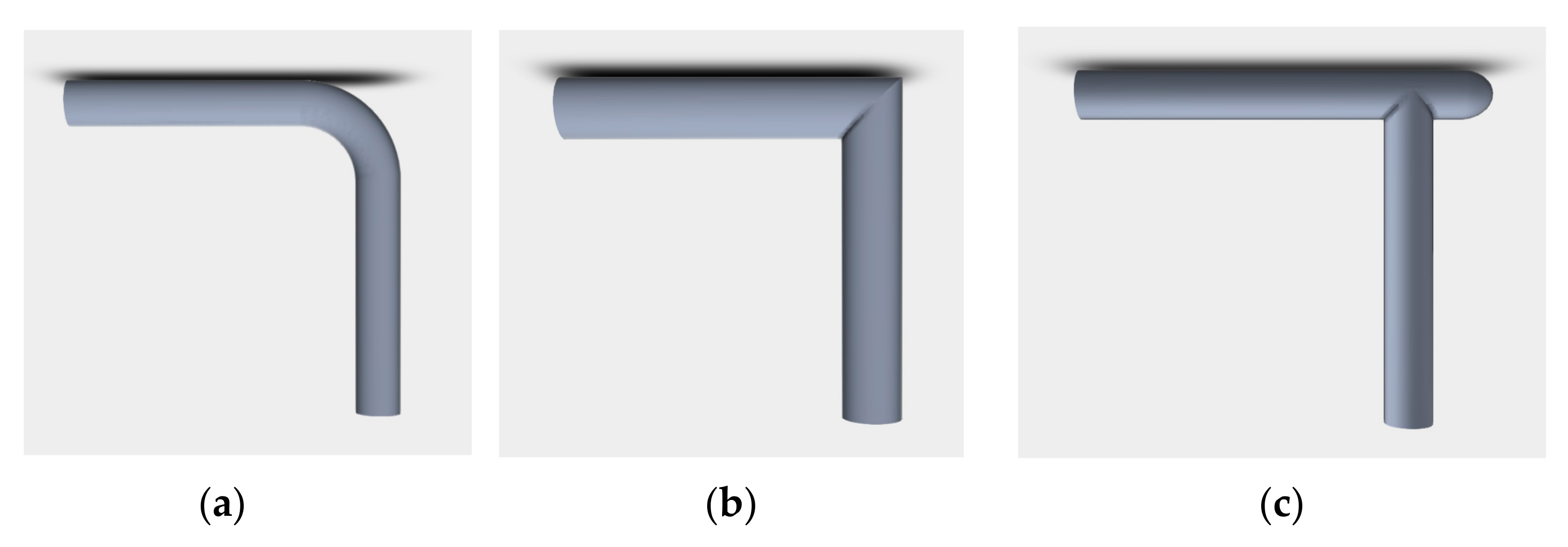
3.1. Geometric Model

Three typical elbow structures, 90° elbow, right-angle elbow. and blind tee, which are widely used in the actual gathering pipeline network, were selected for numerical simulation of erosion. The geometric models of 90° elbow, right-angle elbow, and blind tee were established by selecting 80 mm pipe diameter, as shown in Figure 2.

The above main research objects are seamless steel pipe and elbow, while the pipeline is welded from different pipe segments in the actual engineering. Hence, the erosion rate simulation study is also done on the weld seam of straight pipe and elbow pipe in the engineering. The diameter of 80 mm and 150 mm was selected, and the weld seam was set to 2.5 mm high and 1 mm wide, according to the data provided in the field. The geometric models of the two weld structures of the straight pipe weld and the bend weld were established respectively, as shown in Figure 3.

For all the above geometries, ICEM CFD is used to extract and mesh the computational domain of the established geometric model, and a non-structural mesh is adopted. The inner flow channel is selected as the calculation domain to simulate the gas flow. In order to simulate the boundary layer effect and make the mesh and surface orthogonal, a 3-layer prismatic layer mesh is added to the outer surface of the computational domain. The minimum mesh quality is 0.36, which can be used for CFD calculations. In addition, the standard wall function is used near the wall, and the condition of 30 < y+ < 300 for the first grid cell is set for mesh quality. The stationary wall boundary condition is set as the no-slip. The standard wall roughness model is adopted, the roughness thickness value Ks is set to 0.05 mm, and the roughness constant Cs keeps the default value 0.5, which means that the pipe wall roughness is evenly distributed. In addition, the wall boundary condition type of DPM is set as reflect.

3.2. Parameter Settings

The proposed numerical model above is employed to investigate gas-solid erosion of three typical elbow structures: 90° elbow, right-angle elbow, and blind tee in a shale gas field. The influence of six important factors on the maximum erosion rate was studied. The values of these factors were determined according to the actual production and operation conditions, as shown in

Table 2. Parameters of influencing factor.

Influencing Factors	Variable Value
Gas flow rate (m/s)	1/2/3/4/5/6/7
Sand mass flow (kg/s)	0.001/0.0008/0.0006/0.0004/0.0002/0.0001
Sand particle size (μm)	60
Inner diameter (mm)	80/150
Curvature radius of elbow	1.5D/3D
Structure type	90° elbow/right angle elbow/blind tee
Weld type	straight pipe weld/elbow weld

.

ANSYS Fluent software is employed for steady-state calculation. The Pressure-Based solver based on the SIMPLE algorithm is used for pressure-velocity coupling. The convergence criterion of the calculation result is that the residual amount of each governing equation is less than 0.001. The number of iterations is 1000. In addition, the steady-state calculation is performed, so the governing equations for the pressure-based solver do not contain time-dependent terms. The CFL number is calculated by the sub-relaxation factor, and the default sub-relaxation factor value in Fluent is used. The default values of the sub-relaxation factor for pressure, momentum, turbulent kinetic energy k, and dissipation rate e are 0.3, 0.7, 0.8, and 0.8, respectively.

The quality of the grid directly affects the accuracy and speed of the calculation, in general, the dense grid improves the accuracy of the results, but it also requires more computer resources. Mesh independent verification is carried out on each geometric structure. The mesh system with a mesh quantity of 316,649 is selected.

4. Results and Discussion

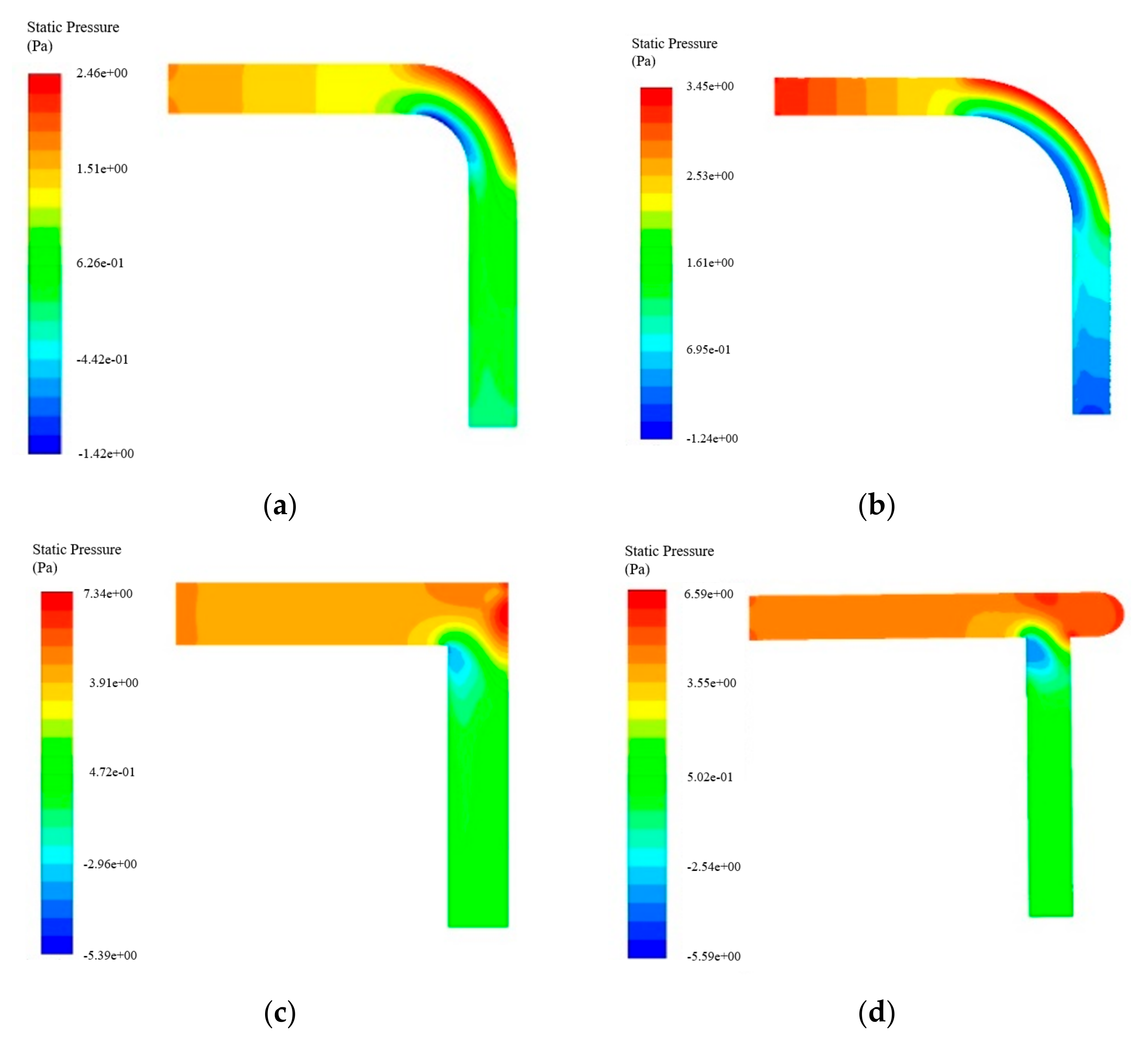
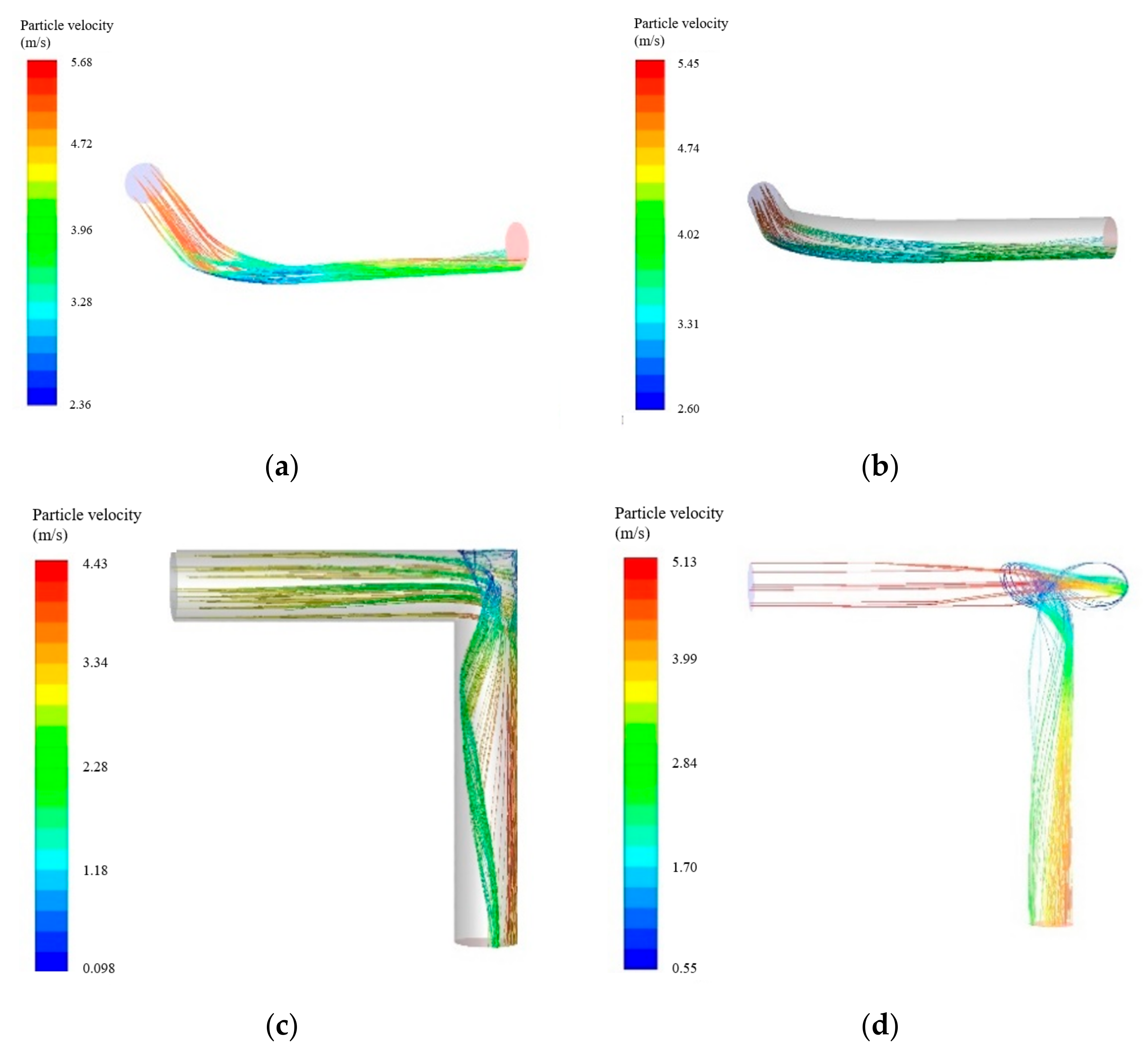
4.1. Erosion Analysis of Right Angle/Elbow/Blind Tee

The maximum erosion rates of the pipe wall under different incident velocities and different sand mass flow rates were simulated and calculated respectively under the condition that other influencing factors were fixed (pipe diameter 80 mm, sand diameter 60 μm). The mass flow rate and gas velocity of the particles were fixed at 0.001 kg/s and 7 m/s, respectively. The trends of different bend structures with gas velocity and mass flow rate were compared, as shown in Figure 4.

As can be seen from Figure 4, the maximum erosion rate of the pipe wall increases exponentially with the increase of the gas velocity. The exponential growth rate of the blind tee is the most obvious, and the erosion rates of 1.5D elbow, 3D elbow, and right-angle elbow are close to each other. The maximum erosion rate of the right-angle elbow is slightly larger than that of the 90° elbow when the gas velocity is below 5 m/s, and when the gas velocity is greater than or equal to 5 m/s, the maximum erosion rate of the right-angle elbow is smaller. The maximum erosion rate of the pipe wall increases linearly with the increase of sand mass flow rate, and the maximum erosion rate of the blind tee is the largest and fastest, while the maximum erosion rate of the right-angle elbow is the smallest.

Figure 5, Figure 6 and Figure 7 show the detailed flow field information. As can be seen from Figure 5, Figure 6 and Figure 7, the flow direction has changed abruptly at the 90° elbow of the right-angle bend. Due to the compression of the outside fluid, the fluid near the inside diffuses, resulting in the generation of vortex flow at the bend; simultaneously, the flow velocity distribution is seriously uneven, and at the 90° elbow near the outside wall, the pressure rises sharply, the corresponding flow velocity decreases sharply. There is an obvious low-velocity zone, while the center and the inner region is a low-pressure, high-velocity zone, respectively. The flow field path lines show the formation of vortices. The airflow in the downstream tube of the bend shows a certain spiral flow pattern. The distribution of erosion area is related to the flow state. Compared with the elbow, the flow field near the blind end in the tee is complex, and the particles will rebound to the upstream, so the severely impacted areas are dispersed. However, due to the high energy of particles impacting the wall, the erosion rate at the most serious point of erosion is high. Near the 90° bend, the solid particles directly collide with the outer side of the back section of the bend, and wall erosion occurs, forming an erosion wear area with a concentrated area and the largest amount of erosion. In the flow separation area, some solid particles rebound from the wall surface and collide with the inner side of the downstream pipe wall, but the rebound speed is significantly reduced, so the erosion is not obvious. The maximum erosion rate of the 3D elbow is obviously smaller than that of the 1.5D elbow. Therefore, in the production practice, the elbow with a large curvature radius should be selected to reduce the erosion wear at the elbow.

This paper mainly focuses on the movement of particles and the erosion rate on the wall. The pressure drops, pressure coefficient, and so on can be obtained after the simulation. The pressure drops of the 1.5D elbow, 3D elbow, right-angle elbow, and blind tee are 1.71 pa, 3.38 pa, 5.39 pa, and 5.65 pa, respectively. We provide contours of pressure to intuitively show the changes of the pressure field, such as Figure 6.

For the blind tee, part of the incoming flow directly into the blind end due to inertia, and part of the gas flows out from the blind end to the downstream. In the blind end area, the flow field is more complex. There are different degrees of vortex phenomenon among which the blind end is more significant and has a larger effect range. Because the blind end area does not have an outlet, the fluid flow velocity is reduced, and a high-pressure area is formed at the blind end. At the T-junction, the fluid velocity and flow direction change dramatically, and the outer fluid velocity is low while the inner fluid velocity is high. After passing through the T-junction, the fluid velocity in the downstream straight section gradually becomes uniform. From the trajectory nephogram of solid particles, it can be seen that most of the particles entering at the inlet enter the blind end area directly due to inertia, and these particles collide directly with the wall of the blind end and subsequently rebound. Due to some factors, such as the opposite direction to the airflow and the collisional energy dissipation of the inlet inflow particles, the particle velocity is greatly reduced after the rebound. A large number of vortices generate at the blind end, so the residence time of particles at the blind end is prolonged. The particles may collide with the wall of the blind end several times, resulting in increased energy dissipation of the particles. Therefore, particles are very easy to gather at the blind end, forming a particle accumulation layer. Another part of the particles flows directly downstream with the airflow, with low-velocity energy loss. The vortex effect makes most of the particles concentrate near the blind end area, which causes the velocity energy and the number of particles entering the downstream pipeline from this area to become smaller. From the erosion rate graph, we can see that the most serious erosion is at the wall of the blind end. When using blind tees in actual projects, attention should be paid to the design of the wall thickness at the blind end, sufficient allowance for erosion should be considered, and erosion testing should be carried out regularly at the blind end to avoid the formation of safety hazards.

4.2. Erosion Analysis of 1.5D/3D Elbow Erosion

The curvature radius of 90° bends used in the gas field are mostly 1.5D and 3D, so we focus on comparing the erosion of these two different curvature radii under the gas field conditions. Under the condition that other influencing factors are certain (90° bend, pipe diameter 80 mm, sand diameter 60 μm), the simulated flow velocity range is determined according to the actual field conditions, and the flow velocity is taken from 1 m/s to 7 m/s, the simulated sand mass flow rate is taken from 0.0001 kg/s to 0.001 kg/s. The maximum erosion rates of the pipe wall under the simulated conditions are shown in Figure 8.

From Figure 8, it can be seen that the trend of the maximum erosion rate of the tube wall is approximately the same in the 1.5D and 3D cases, and the variation area of the maximum erosion rate of the tube wall is nearly the same in both turning radii. There is an interesting phenomenon in Figure 8 that the erosion rate difference between 3 m/s and 4 m/s is small, but a big difference occurs from 5 m/s. This is because there is a nonlinear relationship between velocity and erosion rate according to Equation (10). Therefore, when the flow velocity is low, the maximum erosion rate increases relatively slowly with the increase of flow velocity. Fixing the mass flow rate and gas velocity of particles at 0.001 kg/s and 7 m/s, respectively, the trend of the wall erosion rate with the gas velocity and mass flow rate in the 1.5D and 3D cases are compared as shown in Figure 9. As can be seen from Figure 9, the maximum erosion rate of the pipe wall increases exponentially with the increase of the gas velocity, and the maximum erosion rate of the inner wall of the 1.5D elbow is slightly larger than that of the 3D elbow; the maximum erosion rate of the pipe wall increases linearly with the increase of the sand mass flow rate. In addition, the maximum erosion rate of the inner wall of the 1.5D elbow is larger than that of the 3D elbow on the whole.

As shown in Figure 5a,b and Figure 7a,b, with the increase of bend radius, the bending path becomes longer and the erosion area becomes larger but the erosion degree is weakened. When the bend radius is 3D, the particles collide with the wall twice at the bend, resulting in a larger erosion area; while the bend radius is 1.5D, the particles collide with the wall more intensively, so the erosion area is more concentrated. As the curvature radius of the 1.5D bend is smaller, the particles change direction faster when passing through the bend, while the particles change speed more smoothly when passing through the 3D bend. Therefore, the maximum erosion rate of the 1.5D bend is larger than that of 3D bend, while the erosion of the 3D bend affects a wider area.

As can be seen in Figure 6a,b, it can be observed that the gas pressure inside the small curvature radius elbow decreases faster after passing the turning place. The pressure difference makes the speed of the particles faster when passing the elbow, resulting in the particles collide with the inner surface of the elbow faster. In contrast, the pressure change inside the large curvature radius elbow is smoother, and the velocity change process is relatively smoother when the particles pass through the large curvature radius elbow. It can also be concluded that the maximum erosion rate of the small curvature radius elbow is greater than that of the large curvature radius elbow.

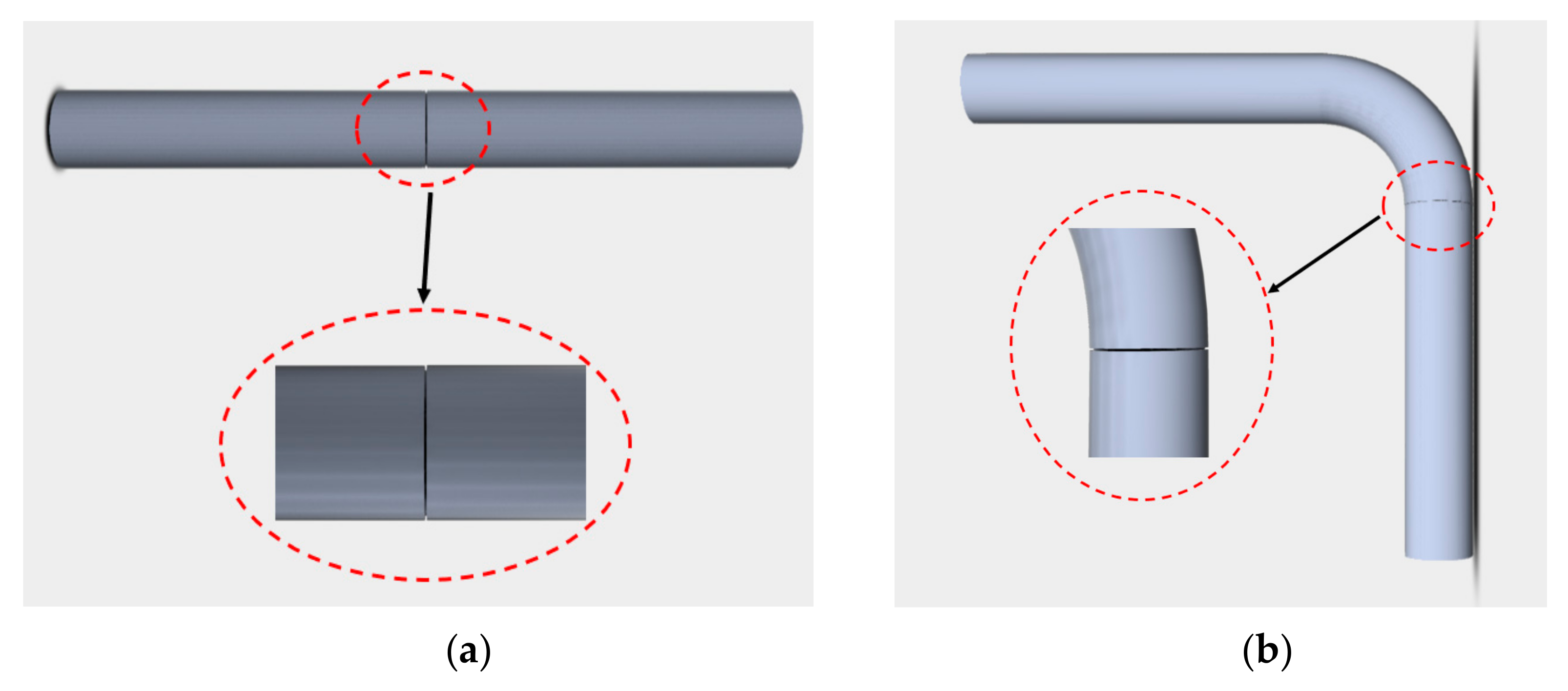
4.3. Erosion Analysis of Straight Pipe Weld/Elbow Weld

The maximum erosion rates of straight and elbow welds under different gas velocities and sand mass flow rates were simulated under the condition that other influencing factors were fixed (pipe diameter 80 mm, sand diameter 60 μm). The variation trends of different weld types with gas velocity and mass flow rate were compared, as shown in Figure 10. Due to the existence of weld, the trajectory of particles in the pipe is complex and changeable, resulting in the inconsistency between the results of individual simulation working conditions and the law of pipe without weld. Therefore, under some working conditions, the maximum erosion rate of pipe wall when the gas flow rate is 5 m/s is greater than that when the gas flow rate is 6 m/s.

As can be seen from Figure 11, the maximum erosion rate of both straight pipe welds and bent pipe welds increases linearly with the increase of mass flow rate, with the erosion rate of bent pipe welds increasing faster. Under the same conditions, the erosion rate of bent pipe welds is much greater than that of straight pipe welds.

From Figure 12, it can be seen that the maximum erosion rates of both the straight pipe and the bent pipe are located in the weld seam. Due to the consideration of gravity, the number of particles in the lower part of the straight pipe is greater than the upper part, so the maximum erosion rate of the straight pipe weld is located in the lower part of the weld; while in the bent pipe, due to the pressure difference between the inner and outer sides of the inner wall of the bend and the inertia of the particles, the particle velocity as well as the particle density on the outer side of the bend is much greater than that on the inner side. Therefore, the position of maximum erosion rate of the bend weld is located in the weld on the outer side of the inner wall of the bend.

The pressure distribution of different welds is shown in Figure 13, which indicates that there is an obvious difference between the pressure inside the straight pipe and the bend before and after the weld. Due to the fact that the weld is equivalent to a small throttling device, the velocity of the gas suddenly increases when passing through the weld, resulting in a large pressure difference before and after the weld. Under the effect of pressure difference, the collision speed of particles with the weld increases, and the erosion rate is also greater when particles pass through the weld. It can be seen that the weld is also a part of the pipeline which is easy to be eroded. Welding operation should be carried out in strict accordance with the engineering specifications during construction. Meanwhile, regular erosion detection should be carried out on the weld to avoid the formation of safety risks.

Figure 14 shows the comparison of an elbow pipe without welding and an elbow pipe with welding. It can be seen that for pipe fittings of the same specification, the maximum erosion rate of elbows with welds is larger. This is because the existence of the weld will greatly increase the probability of the weld colliding with solid particles.

5. Conclusions

In this paper, steady state numerical simulations were conducted for 1.5D elbow, 3D elbow, right angle elbow and blind tee under gas field conditions to investigate the flow field characteristics and the erosion law of particles. An integrated CFD-DPM method is established including realizable k-ε turbulence model, discrete phase model, and erosion rate prediction model.

(1)

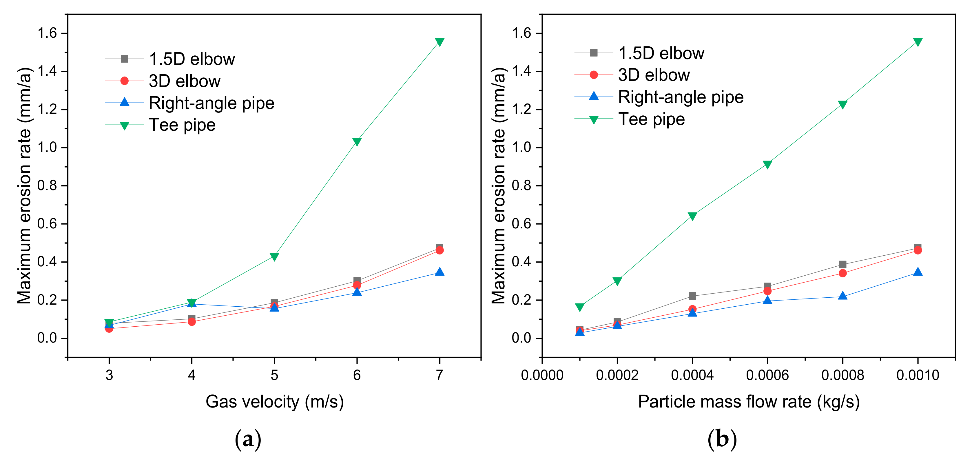
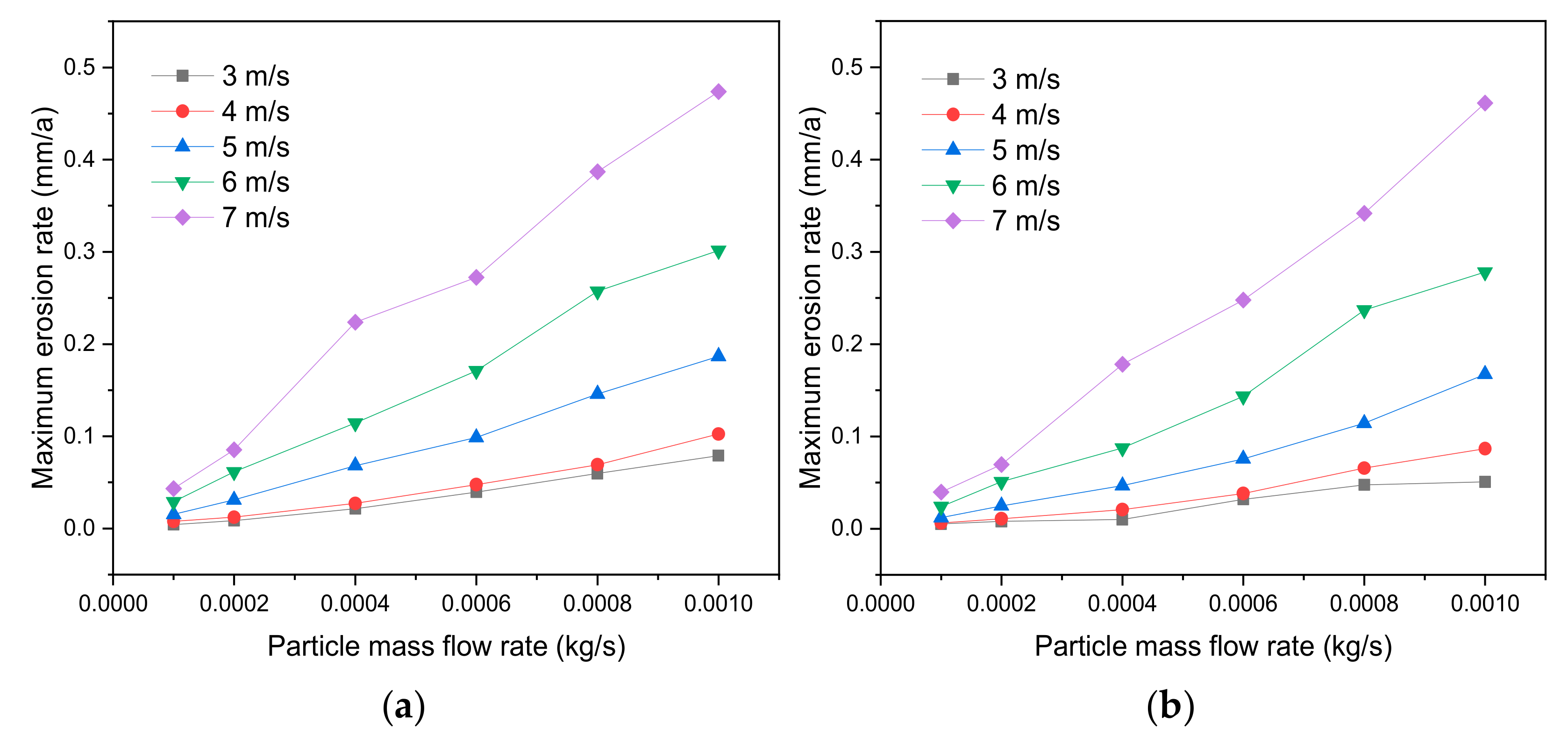
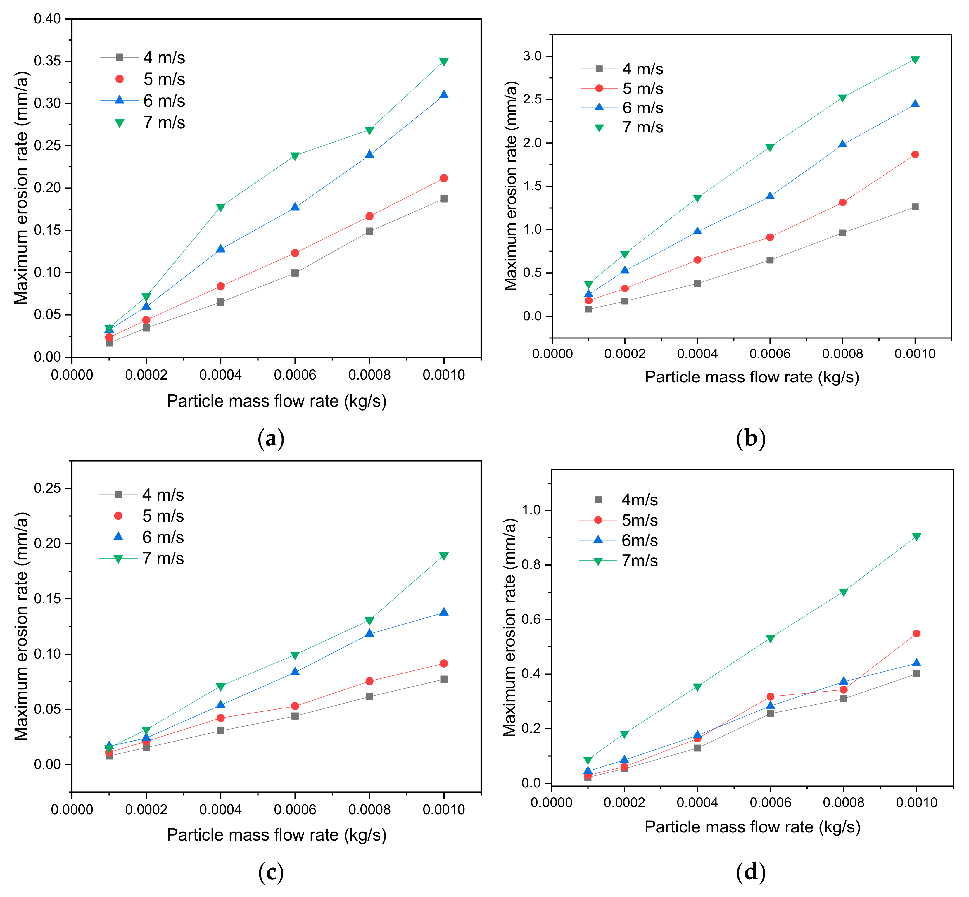
The maximum erosion rate of the pipe wall is positively nonlinear with the incident velocity and increases linearly with the increase of sand mass flow rate. The blind tee has the most obvious growth rate followed by the erosion rates of 1.5D elbow and 3D elbow, while the maximum erosion rate of the right-angle elbow is the smallest.

(2)

The most serious erosion of the blind tee is located in the blind end of the pipe wall. Compared with elbows, the flow field near the blind end of the tee is complicated, and particles will rebound to the upstream, thereby dispersing the severely affected area. However, due to the high energy of the particles hitting the wall, the erosion rate is high at the point where the erosion is most severe. When using blind tees in actual engineering, attention should be paid to the design of the blind end wall thickness, sufficient erosion margin should be considered, and erosion tests should be carried out on the blind end regularly to avoid potential safety hazards.

(3)

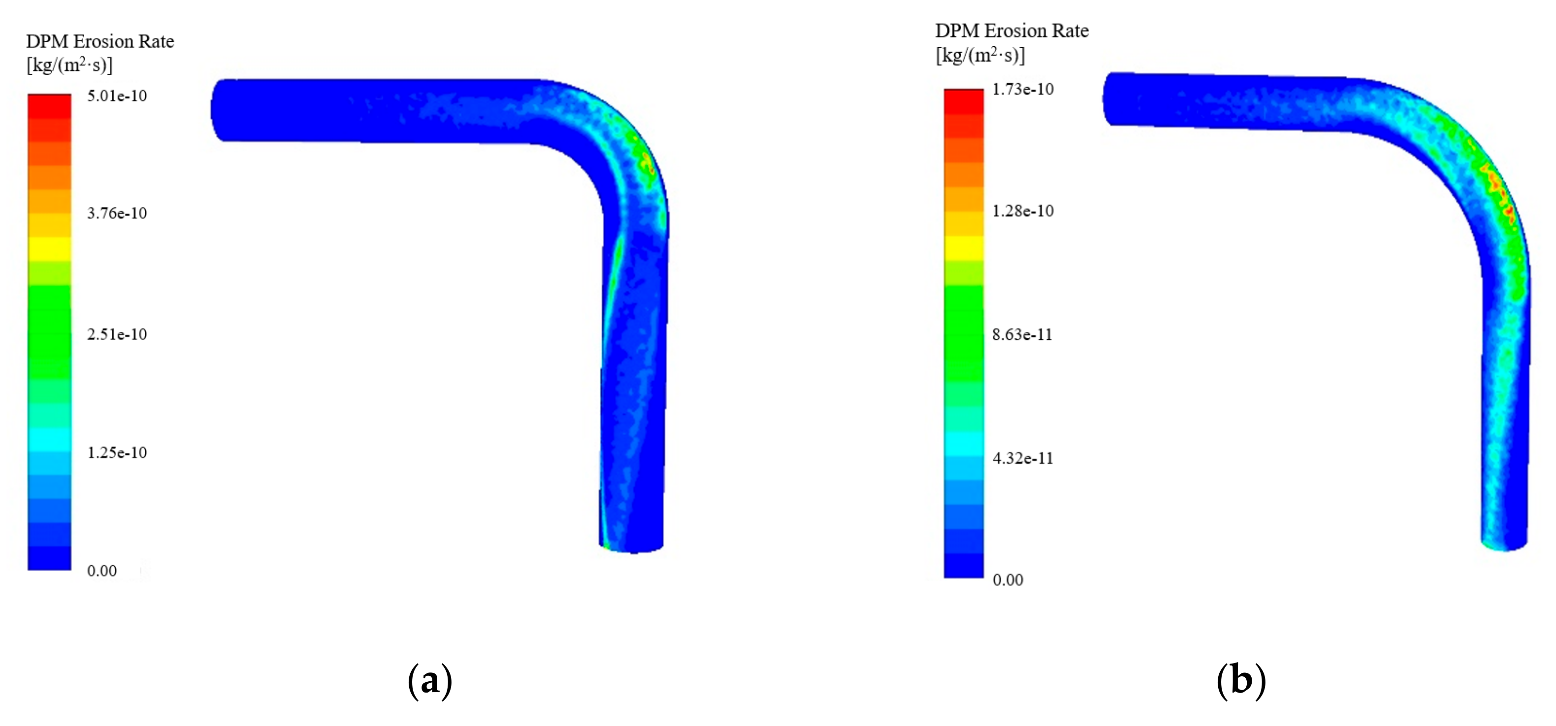
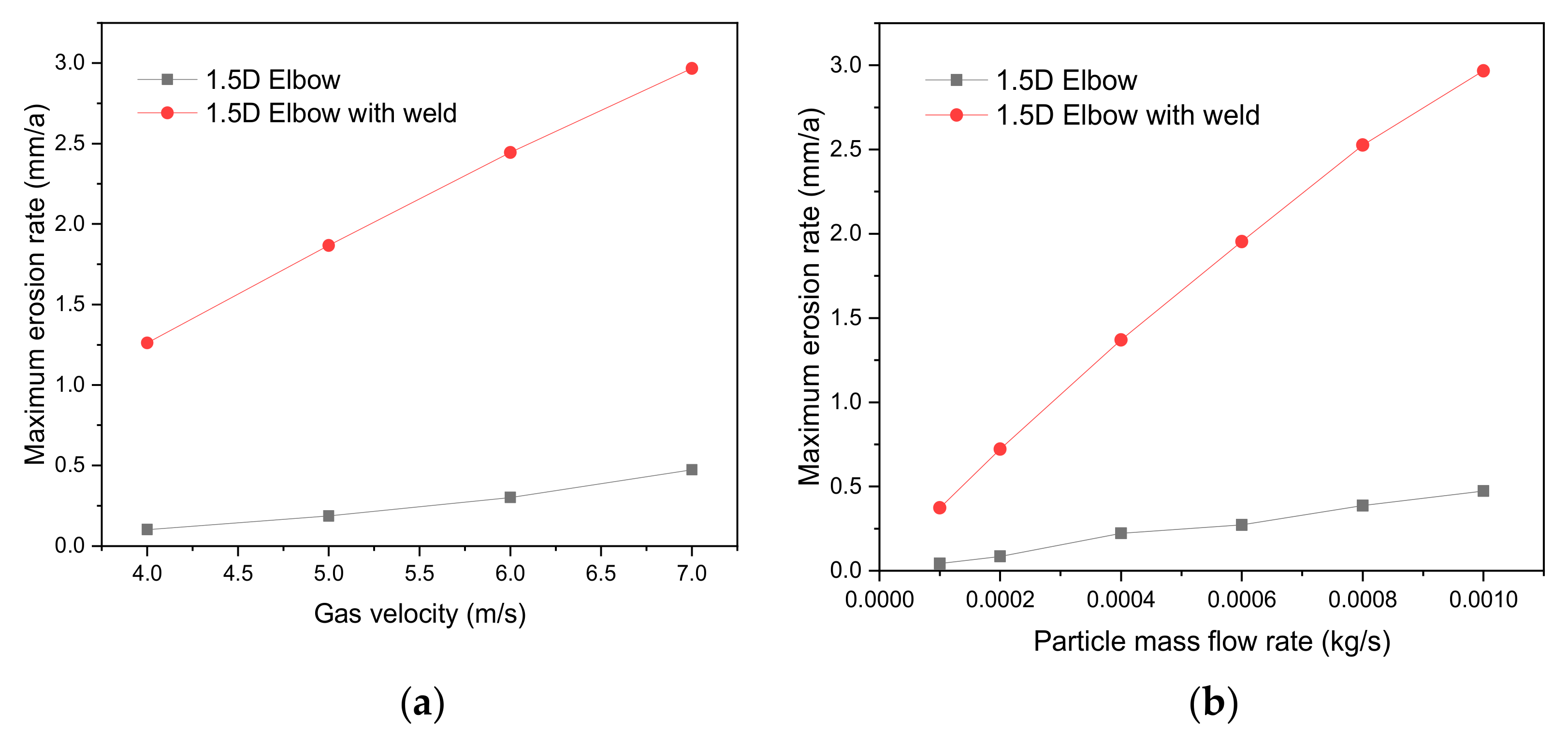
The most serious erosion area of the right-angle elbow is located outside of the downstream pipe wall. The maximum erosion rate of the inner wall of the elbow tube of 1.5D is greater than that of the 3D elbow as a whole, and the 1.5D elbow is more concentrated in the serious erosion area. Therefore, in the production practice, the elbow with a large curvature radius should be selected to reduce the erosion wear at the elbow.

(4)

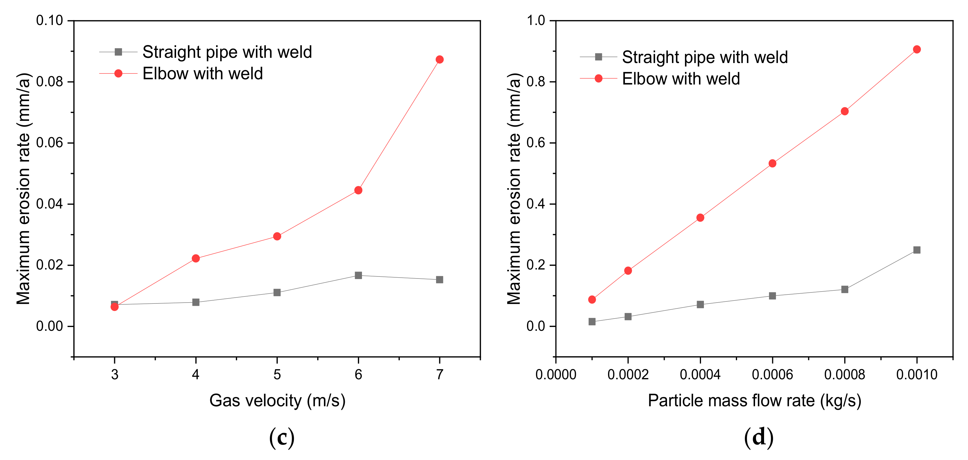
The maximum erosion position of the straight pipe weld is located in the near-ground part of the weld due to gravity, and the maximum erosion rate of the bend weld is located in the weld on the outside of the inner wall of the bend. Under the same conditions, the erosion rate of the bend weld is much greater than that of the straight pipe weld, and the increasing trend is more obvious with the increase of the incidence speed and mass flow rate of sand particles.

(5)

For pipe fittings of the same specification, the maximum erosion rate of elbows with welds is larger than without welds. The weld is a part of the pipeline that is prone to erosion. Therefore, the welding operation must be carried out in strict accordance with the engineering specifications during the construction.

References

1. Hong, B.; Li, X.; Song, S.; Chen, S.; Zhao, C.; Gong, J. Optimal planning and modular infrastructure dynamic allocation for shale gas production. Appl. Energy 2020, 261. [Google Scholar] [CrossRef]
2. Peng, S.; Chen, Q.; Shan, C.; Wang, D. Numerical analysis of particle erosion in the rectifying plate system during shale gas extraction. Energy Sci. Eng. 2019, 7, 1838–1851. [Google Scholar] [CrossRef]
3. Hong, B.; Li, X.; Li, Y.; Li, Y.; Yu, Y.; Wang, Y.; Gong, J.; Ai, D. Numerical Simulation of Elbow Erosion in Shale Gas Fields under Gas-Solid Two-Phase Flow. Energies 2021, 14, 3804. [Google Scholar] [CrossRef]
4. Parsi, M.; Najmi, K.; Najafifard, F.; Hassani, S.; McLaury, B.S.; Shirazi, S.A. A comprehensive review of solid particle erosion modeling for oil and gas wells and pipelines applications. J. Nat. Gas Sci. Eng. 2014, 21, 850–873. [Google Scholar] [CrossRef]
5. Hong, B.; Li, X.; Di, G.; Song, S.; Yu, W.; Chen, S.; Li, Y.; Gong, J. An integrated MILP model for optimal planning of multi-period onshore gas field gathering pipeline system. Comput. Ind. Eng. 2020. [Google Scholar] [CrossRef]
6. Andrews, D.R. An analysis of solid particle erosion mechanisms. J. Phys. D. Appl. Phys. 1981, 14, 1979–1991. [Google Scholar] [CrossRef]
7. Chen, X.; McLaury, B.S.; Shirazi, S.A. A comprehensive procedure to estimate erosion in elbows for gas/liquid/sand multiphase flow. J. Energy Resour. Technol. Trans. ASME 2006, 128, 70–78. [Google Scholar] [CrossRef]
8. Kang, R.; Liu, H. An integrated model of predicting sand erosion in elbows for multiphase flows. Powder Technol. 2020, 366, 508–519. [Google Scholar] [CrossRef]
9. Farokhipour, A.; Mansoori, Z.; Saffar-Avval, M.; Ahmadi, G. 3D computational modeling of sand erosion in gas-liquid-particle multiphase annular flows in bends. Wear 2020, 450–451, 203241. [Google Scholar] [CrossRef]
10. Ferng, Y.M.; Lin, B.H. Predicting the wall thinning engendered by erosion-corrosion using CFD methodology. Nucl. Eng. Des. 2010, 240, 2836–2841. [Google Scholar] [CrossRef]
11. Zhu, H.; Lin, Y.; Zeng, D.; Zhou, Y.; Xie, J.; Wu, Y. Numerical analysis of flow erosion on drill pipe in gas drilling. Eng. Fail. Anal. 2012, 22, 83–91. [Google Scholar] [CrossRef]
12. Messa, G.V.; Wang, Y.; Negri, M.; Malavasi, S. An improved CFD/experimental combined methodology for the calibration of empirical erosion models. Wear 2021, 476, 203734. [Google Scholar] [CrossRef]
13. Alghurabi, A.; Mohyaldinn, M.; Jufar, S.; Younis, O.; Abduljabbar, A.; Azuwan, M. CFD numerical simulation of standalone sand screen erosion due to gas-sand flow. J. Nat. Gas Sci. Eng. 2021, 85, 103706. [Google Scholar] [CrossRef]
14. Bilal, F.S.; Sedrez, T.A.; Shirazi, S.A. Experimental and CFD investigations of 45 and 90 degrees bends and various elbow curvature radii effects on solid particle erosion. Wear 2021, 476, 203646. [Google Scholar] [CrossRef]
15. Duarte, C.A.R.; de Souza, F.J. Innovative pipe wall design to mitigate elbow erosion: A CFD analysis. Wear 2017, 380–381, 176–190. [Google Scholar] [CrossRef]
16. Peng, W.; Cao, X.; Hou, J.; Ma, L.; Wang, P.; Miao, Y. Numerical prediction of solid particle erosion under upward multiphase annular flow in vertical pipe bends. Int. J. Press. Vessel. Pip. 2021, 192, 104427. [Google Scholar] [CrossRef]
17. Ejeh, C.J.; Boah, E.A.; Akhabue, G.P.; Onyekperem, C.C.; Anachuna, J.I.; Agyebi, I. Computational fluid dynamic analysis for investigating the influence of pipe curvature on erosion rate prediction during crude oil production. Exp. Comput. Multiph. Flow 2020, 2, 255–272. [Google Scholar] [CrossRef] [Green Version]
18. Laín, S.; Sommerfeld, M. Numerical prediction of particle erosion of pipe bends. Adv. Powder Technol. 2019, 30, 366–383. [Google Scholar] [CrossRef]
19. Parsi, M.; Agrawal, M.; Srinivasan, V.; Vieira, R.E.; Torres, C.F.; McLaury, B.S.; Shirazi, S.A. CFD simulation of sand particle erosion in gas-dominant multiphase flow. J. Nat. Gas Sci. Eng. 2015, 27, 706–718. [Google Scholar] [CrossRef]
20. Ogunsesan, O.A.; Hossain, M.; Iyi, D.; Dhroubi, M.G. CFD Modelling of Pipe Erosion Due to Sand Transport BT. In Numerical Modelling in Engineering; Abdel Wahab, M., Ed.; Springer: Singapore, 2019; pp. 274–289. [Google Scholar]
21. Gosman, A.D.; Ionnides, S.I. Aspects of computer simulation of liquid-fuelled combustors. J. Energy 1983, 7, 482–490. [Google Scholar] [CrossRef]
22. Haider, A.; Levenspiel, O. Drag coefficient and terminal velocity of spherical and nonspherical particles. Powder Technol. 1989, 58, 63–70. [Google Scholar] [CrossRef]
23. Forder, A.; Thew, M.; Harrison, D. A numerical investigation of solid particle erosion experienced within oilfield control valves. Wear 1998, 216, 184–193. [Google Scholar] [CrossRef]
24. Vieira, R.E.; Mansouri, A.; McLaury, B.S.; Shirazi, S.A. Experimental and computational study of erosion in elbows due to sand particles in air flow. Powder Technol. 2016, 288, 339–353. [Google Scholar] [CrossRef]
25. Liu, P.; Wang, Y.; Yan, F.; Nie, C.; Ouyang, X.; Xu, J.; Gong, J. Effects of Fluid Viscosity and Two-Phase Flow on Performance of ESP. Energies 2020, 13, 5486. [Google Scholar] [CrossRef]
Figure 1. Comparison of simulation and experiment results.
Energies 14 06609 g001
Figure 2. Schematic diagram of geometric structure. (a) 90° elbow; (b) Right-angle elbow; (c) Blind tee.
Energies 14 06609 g002
Figure 3. Geometric models of different welds. (a) Straight pipe weld; (b) Elbow pipe weld.
Energies 14 06609 g003
Figure 4. Maximum erosion rate of different pipe component structure. (a) Particle mass flow rate 0.001 kg/s; (b) Gas velocity 7 m/s.
Energies 14 06609 g004
Figure 5. Contours of erosion rate distribution. (a) 1.5D elbow; (b) 3D elbow; (c) Right angle elbow; (d) Blind tee.
Energies 14 06609 g005aEnergies 14 06609 g005b
Figure 6. Contours of pressure. (a) 1.5D elbow; (b) 3D elbow; (c) Right angle elbow; (d) Blind tee.
Energies 14 06609 g006
Figure 7. Particle trajectories. (a) 1.5D elbow; (b) 3D elbow; (c) Right angle elbow; (d) Blind tee.
Energies 14 06609 g007
Figure 8. Maximum erosion rate. (a) 1.5D elbow; (b) 3D elbow.
Energies 14 06609 g008
Figure 9. Maximum erosion rate. (a) Particle mass flow rate 0.001 kg/s; (b) Gas velocity 7 m/s.
Energies 14 06609 g009
Figure 10. Erosion rate of different weld. (a) Straight pipe weld DN80; (b) Bend pipe weld DN80; (c) Straight pipe weld DN150; (d) Bend pipe weld DN150.
Energies 14 06609 g010
Figure 11. Erosion rate of different weld. (a) DN80, 0.001 kg/s; (b) DN80, 7 m/s; (c) DN150, 0.001 kg/s; (d) DN150, 7 m/s.
Energies 14 06609 g011aEnergies 14 06609 g011b
Figure 12. Contours of erosion distribution of different weld. (a) Straight pipe weld; (b) Bend pipe weld; (c) Straight pipe weld (local enlargement); (d) Bend pipe weld (local enlargement); (e) Straight pipe weld particle trajectory; (f) Bend pipe weld particle trajectory.
Energies 14 06609 g012aEnergies 14 06609 g012b
Figure 13. Contours of pressure distribution of different welds. (a) Straight pipe weld; (b) Bend pipe weld.
Energies 14 06609 g013
Figure 14. Erosion rate of DN80, 1.5D elbow pipe without welding and with welding. (a) 0.001 kg/s; (b) 7 m/s.
Energies 14 06609 g014