PSO Self-Tuning Power Controllers for Low Voltage Improvements of an Offshore Wind Farm in Taiwan

Abstract

A de-loaded real power control strategy is proposed to decrease the real power output and increase the reactive power output of a grid-connected offshore wind farm in order to improve the voltage profile when the wind farm is subject to a grid fault. A simplified linear model of the wind farm is first derived and a fixed-gain proportional-integral (PI) real power controller is designed based on the pole-zero cancellation method. To improve the dynamic voltage response when the system is subject to a major disturbance such as a three-phase fault in the grid, a self-tuning controller based on particle swarm optimization (PSO) is proposed to adapt the PI controller gains based on the on-line measured system variables. Digital simulations using MATLAB/SIMULINK were performed on an offshore wind farm connected to the power grid in central Taiwan in order to validate the effectiveness of the proposed PSO controller. It is concluded from the simulation results that a better dynamic voltage response can be achieved by the proposed PSO self-tuning controller than the fixed-gain controller when the grid is subject to a three-phase fault. In addition, low voltage ride through (LVRT) requirements of the local utility can be met by the wind farm with the proposed power controller.

1. Introduction

According to the nuclear-free energy policy in Taiwan, more than 20% of the electrical energy will come from renewable energy by 2025. Furthermore, the installed capacities of the island and offshore wind farms will reach 1.2 GW and 5.7 GW, respectively. With the increasing percentage of wind power generation, how to improve the fault ride through (FRT) capability of a wind farm when it is subject to a grid fault very close to the wind farm has received much attention in recent years [1].

Doubly fed induction generators (DFIGs) have been widely employed for wind energy conversion due to their variable speed operation capability, low converter cost, and independent controllability of real and reactive power. However, the DFIG is sensitive to grid voltage variations as its stator is directly connected to the grid [2,3,4]. Numerous papers have been published to protect the DFIG and the power electronic devices in the rotor side converter (RSC) and grid side converter (GSC) from over-current and over-voltage under disturbance conditions [5,6,7,8,9,10,11,12,13,14,15,16,17,18,19,20,21]. A rotor side crowbar circuit [5,6] has been proposed to divert transient rotor over-currents to prevent the RSC power semiconductor devices from being damaged under grid fault conditions. A DC-link brake chopper across the converter dc link was presented in [7] to ensure satisfactory dc link voltage during a fault. In [8], a series dynamic resistor (SDR) combined with a crowbar resistor and a DC-link brake chopper was designed. A proper value for the SDR was derived. A series voltage compensator in the stator was proposed in [9] to provide the required compensation voltage such that rotor over-current could be avoided. In [10], a dc-link chopper-controlled braking resistor and a series dynamic braking resistor were studied. A passive resistive network consisting of shunt and series elements was installed at the stator [11,12] in order to achieve grid-fault tolerant operation. In [13], a protection scheme using series dynamic braking resistor was proposed to reach a desirable terminal voltage under voltage dip conditions. Grid side dynamic voltage restorers have been proposed in [14,15,16,17] to avoid rotor over-current and provide voltage support for the stator voltage. Although the aforementioned works are effective in protecting the DFIG and the associated power electronic devices under grid fault conditions, additional hardware components are required in order to implement these fault ride through techniques.

Another way to attain an improved fault ride through operation of DFIG is the software improvement and control algorithm method which requires no additional cost. In [22], a virtual damping strategy was proposed to control the stator transient flux under disturbance conditions. A control strategy that temporarily stored the output power in the generator rotor during grid faults was presented in [23] in which a pitch angle control was activated when the rotor speed exceeds its upper limit. In [24], a fuzzy controller was designed to control the real and reactive powers of the wind farm in order to maintain constant voltage at the point of common coupling (PCC). An optimal controller designed using a genetic algorithm was proposed in [25] to prevent over-currents during faults.

In this paper, a novel de-loaded power control algorithm without additional hardware components is proposed to improve the terminal voltage and to increase the reactive power output of a DFIG subject to grid faults. When a low voltage is detected at the DFIG stator, the real power command $P_e^{*}$ is de-loaded from maximum power point tracking (MPPT) value to a level proportional to terminal voltage. After a simplified linear model of the wind farm is derived, a fixed-gain proportional-integral power controller is designed based on pole-zero cancellation method to yield the desired quadrature axis (q-axis) rotor current command $i_{qr}^{*}$ from the real power command. To prevent rotor current from overloading, the direct axis (d-axis) rotor current command $i_{dr}^{*}$ is selected such that the rotor current is equal to its rated value (1 pu). By decreasing the real power command $P_e^{*}$ and q-axis rotor current command $i_{qr}^{*}$, the d-axis rotor current command $i_{dr}^{*}$ and the reactive power output of DFIG can be increased. As a result, the terminal voltage is improved. Since the gains for the fixed-gain proportional-integral (PI) controllers have been designed based on a particular operating point, the dynamic responses of the PI controller may deteriorate when there is a drastic change in system variables due to a major disturbance such as a three-phase fault in the grid. In this work, a self-tuning controller based on particle swarm optimization (PSO) [26,27,28] is presented to adapt the real power controller gains $K_p$ and $K_i$ in real-time.

MATLAB/SIMULINK was employed to simulate the dynamic performance of an offshore wind farm connected to the power grid in central Taiwan under grid fault conditions. The simulation results indicate the proposed PSO self-tuning power controller can reach better voltage profile than the fixed-gain PI controller. It is also observed that the wind farm with the proposed controller meets the low voltage ride through (LVRT) requirements of the local utility in Taiwan. Based on the simulation results, it is concluded that a better voltage profile can be achieved by the proposed PSO self-tuning power controller than the fixed-gain PI controller. It is also observed from the simulation results that the wind farm with the proposed controller meets the low voltage ride through (LVRT) requirements of the local utility in Taiwan.

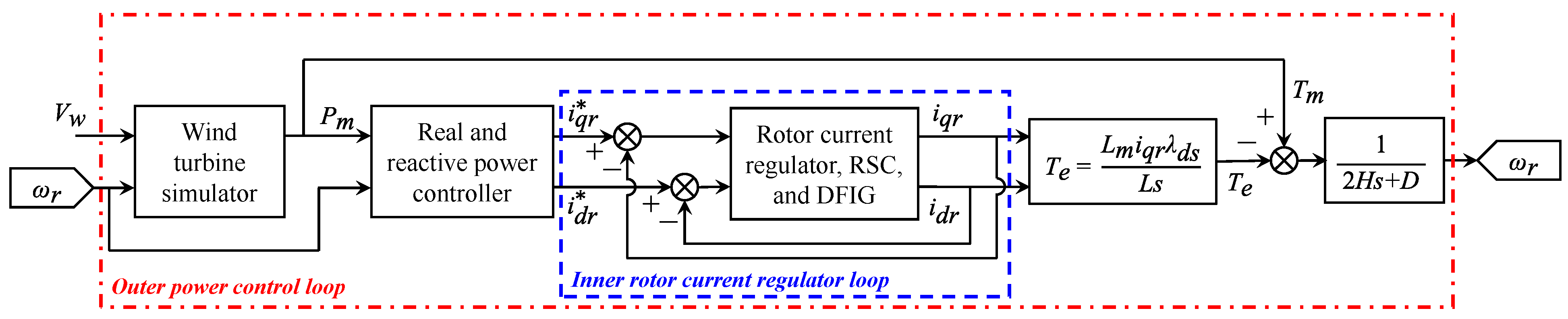
2. System Model

The system under study is an offshore wind farm connected to the utility grid in central Taiwan as shown in Figure 1.

The wind farm comprises 80 wind generators, each rated 2.5 MW. These wind generators are lumped as an equivalent 200 MW DFIG generator in order to reduce the computational burden of MATLAB/SIMULINK simulations. In addition, the system beyond Chung-Liao South substation is modeled as an infinite bus since its capacity is much higher than the wind farm. As a result, only the portion of the system surrounded by the dashed line in Figure 1 is simulated by MATLAB/SIMULINK.

The real and reactive power outputs of the wind farm are controlled by the RSC. By aligning the d-axis to stator flux linkage, the real power is controlled by the q-axis rotor current $i_{qr}$ while the reactive power is controlled by the d-axis rotor current $i_{dr}$ [29,30].

Figure 2 depicts the functional block diagram for real and reactive power control of a DFIG using a dq-axis rotor current regulator. As shown in Figure 2, a wind turbine simulator is employed to yield the DFIG mechanical torque $T_m$ and mechanical power $P_m$ under the specified wind speed $V_w$ and rotor speed ${\mathsf{\omega }}_r$.

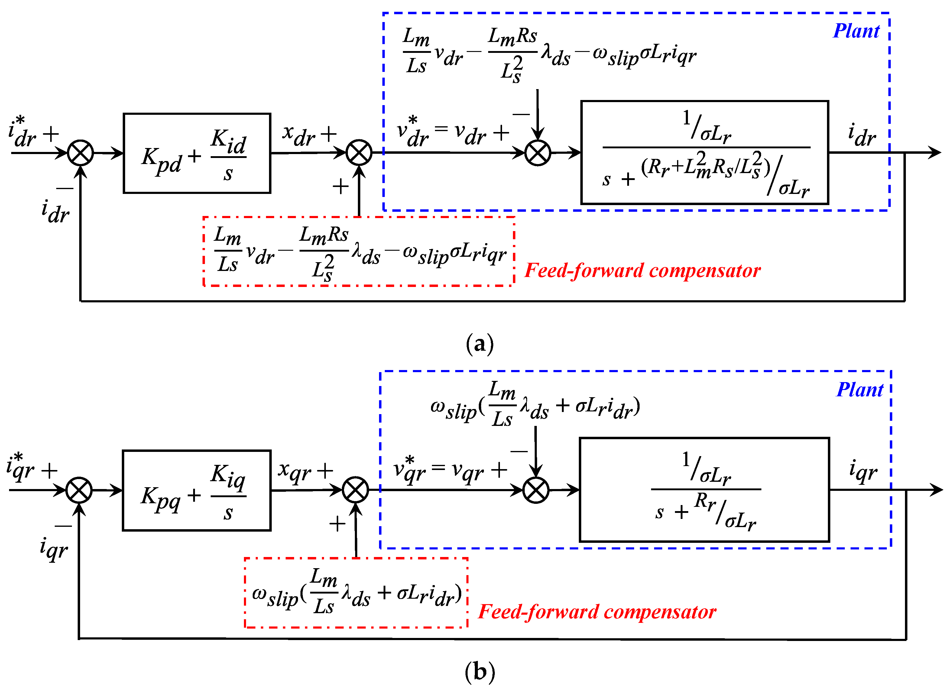
2.1. Non-Linear Model of the Doubly Fed Induction Generator (DFIG) Current Regulator

Under stator flux orientation, the DFIG state equations with stator flux variations being considered can be written as follows [29].

$$\frac{d}{dt}\left[\begin{array}{c}{i}_{dr}\\ i_{qr}\\ {\lambda }_{ds}\end{array}\right]=\left[\begin{array}{ccc}\frac{-(R_r+L_m^2{R}_s/L_s^2)}{\sigma L_r}& {\omega }_{slip}& \frac{L_m{R}_s}{\sigma L_r{L}_s^2}\\ -{\omega }_{slip}& -\frac{R_r}{\sigma L_r}& -\frac{{\omega }_{slip}{L}_m}{\sigma L_r{L}_S}\\ \frac{L_m}{L_S}{R}_s& 0& -\frac{R_s}{L_S}\end{array}\right]\left[\begin{array}{c}{i}_{dr}\\ i_{qr}\\ {\lambda }_{ds}\end{array}\right]+\left[\begin{array}{c}\frac{v_{dr}}{\sigma L_r}-\frac{L_m{v}_{ds}}{\sigma L_r{L}_s}\\ \frac{v_{qr}}{\sigma L_r}\\ v_{ds}\end{array}\right]$$

(1)

To achieve dq-axis decoupling, feed-forward compensators are included in the d-axis and q-axis current regulators as described below:

$$v_{dr}=x_{dr}+\frac{L_m}{L_s}(v_{ds}-\frac{{\lambda }_{ds}}{L_s}{R}_s)-{\omega }_{slip}\sigma L_r{i}_{qr}$$

(2)

$$v_{qr}=x_{qr}+{\omega }_{slip}(\frac{L_m}{L_s}{\lambda }_{ds}+\sigma L_r{i}_{dr})$$

(3)

where $x_{dr}$ and $x_{qr}$ are the d-axis and q-axis control signal from the PI current regulators as shown in Figure 3.

2.2. Non-Linear Model of the Real and Reactive Power Controller

The commands for d-axis and q-axis current regulators, $i_{dr}^{*}$ and $i_{qr}^{*}$, in Figure 3 are determined by the real and reactive power controller as described in Figure 4.

As shown in Figure 4, the real power output command $P_e^{*}$ of the DFIG in normal operation is determined based on MPPT as follows [29]:

$$P_e^{*}=P_{e,opt}^{*}=K_{opt}{\omega }_r^3$$

(4)

where $K_{opt}$ is a constant. When there is a fault in the grid causing a voltage dip at PCC ($\left|V_{PCC}\right| \le 0.8$ pu), the real power output command $P_e^{*}$ is decreased to a level proportional to the voltage at PCC, i.e.,

$$P_e^{*}=P_{e,opt}^{*}{V}_{PCC}=K_{opt}{\omega }_r^3{V}_{PCC}$$

(5)

where $V_{PCC}$ is the PCC voltage per unit. Based on the error ${\mathsf{\Delta }P}_e^{*}$ between the real power output command $P_e^{*}$ and the actual real power output $P_e$, a PI real power controller is proposed to generate the desired q-axis rotor current command $i_{qr}^{*}$. In order to improve the dynamic power and voltage responses under fault conditions, the gains of the PI real power controller are adapted in real time using PSO based on on-line measured wind speed $V_w$, real power $P_e$, PCC voltage $V_{PCC}$, rotor speed ${\mathsf{\omega }}_r$, stator and rotor currents, voltages, and flux linkages. Details on the design of the fixed-gain PI real power controller and PSO self-tuning controller will be described in the following sections.

It is also observed in Figure 4 that the d-axis rotor current command $i_{dr}^{*}$ is usually set to be zero [29] in order for the DFIG to have the largest q-axis rotor current command $i_{qr}^{*}$ and maximum real power output as the following constraint must be satisfied by the two rotor current commands $i_{dr}^{*}$ and $i_{qr}^{*}$:

$$i_{dr}^{*}{}^2+i_{qr}^{*}{}^2\le {\left|i_r{}_{,\max }\right|}^2=1$$

(6)

When there is a fault causing a voltage dip, the real power output command $P_e^{*}$ and the resultant q-axis rotor current command $i_{qr}^{*}$ are decreased and the d-axis rotor current command $i_{dr}^{*}$ is increased to a level as described below:

$$i_{dr}^{*}=\sqrt{1-{(i_{qr}^{*})}^2}$$

(7)

Thus, by increasing the d-axis rotor current according to Equation (7), the DFIG reactive power output can be increased and the voltage at PCC can be improved under fault conditions.

3. Design of Fixed-Gain Real Power Controllers

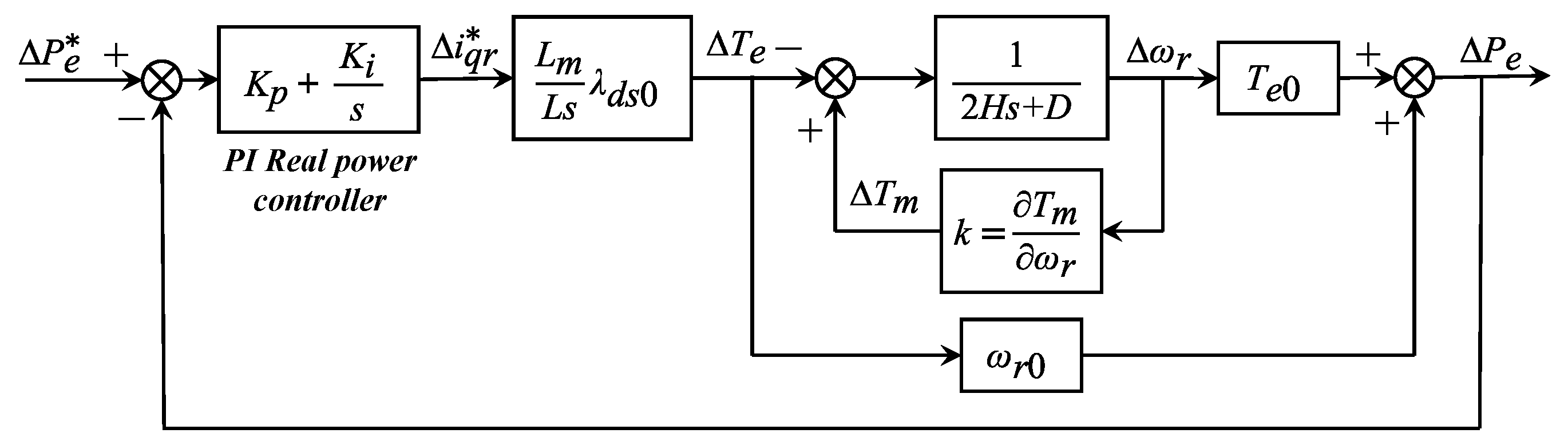
3.1. Linearized Model of the DFIG Gain Real Power Controller

In the design of the fixed-gain real power controller, the non-linear power equation $P_e{=T}_e{\mathsf{\omega }}_r$ is first linearized as follows:

$$\Delta P_e(s)=T_{e0}\Delta {\omega }_r(s)+{\omega }_{r0}\Delta T_e(s)$$

(8)

where the rotor speed deviation can be derived from the block diagram in Figure 2 as follows:

$$\Delta {\omega }_r(s)=(\frac{1}{2Hs+D})(\Delta T_m(s)-\Delta T_e(s))$$

(9)

The increment in mechanical torque can be estimated using the following formula:

$$\Delta T_m(s)=\frac{\partial T_m}{\partial {\omega }_r}\Delta {\omega }_r(s)=k\Delta {\omega }_r(s)$$

(10)

Note that the constant k can be estimated from the wind turbine mechanical torque using the curve fitting technique around the maximum power point [28].

The increment in stator flux linkage, ${\mathsf{\Delta }\mathsf{\lambda }}_{ds}$, can be derived from Equation (1) as follows:

$$\Delta {\lambda }_{ds}(s)=\frac{1}{s+\raisebox{1ex}{$R_s$}\!\left/ \!\raisebox{-1ex}{$L_s$}\right.}(\Delta v_{ds}(s)+\frac{L_m}{L_s}{R}_s\Delta i_{dr}(s))$$

(11)

The electromagnetic torque $T_e$ can be expressed as follows:

$$T_e=\frac{L_m}{L_s}{i}_{qr}{\lambda }_{ds}$$

(12)

By linearizing the torque equation in Equation (12), we get the increment in electromagnetic torque as follows:

$$\Delta T_e(s)=\frac{L_m}{L_s}{\lambda }_{ds0}\Delta i_{qr}(s)+\frac{L_m}{L_s}{i}_{qr0}\Delta {\lambda }_{ds}(s)$$

(13)

From the block diagrams in Figure 3 for d-axis and q-axis current regulators, the following transfer functions can be derived:

$$\frac{\Delta i_{dr}(s)}{\Delta i_{dr}^{*}(s)}=\frac{(K_{pd+}+\frac{K_{id}}{s})\frac{1}{\sigma L_{rs}s+R_r+\raisebox{1ex}{$L_m^2{R}_s$}\!\left/ \!\raisebox{-1ex}{$L_s^2$}\right.}}{1+(K_{pd+}+\frac{K_{id}}{s})\frac{1}{\sigma L_{r}s+R_r+\raisebox{1ex}{$L_m^2{R}_s$}\!\left/ \!\raisebox{-1ex}{$L_s^2$}\right.}}$$

(14)

$$\frac{\Delta i_{qr}(s)}{\Delta i_{qr}^{*}(s)}=\frac{(K_{pq+}+\frac{K_{iq}}{s})\frac{1}{\sigma L_{r}s+R_r}}{1+(K_{pq+}+\frac{K_{iq}}{s})\frac{1}{\sigma L_{r}s+R_r}}$$

(15)

From Equation (7), we obtain:

$$2i_{dr0}^{*}\Delta i_{dr}^{*}+2i_{qr0}^{*}\Delta i_{qr}^{*}=0$$

(16)

Therefore, the increment in d-axis rotor current command $\Delta i_{dr}^{*}$ is related to the increment in q-axis rotor current command $i_{qr}^{*}$ as follows:

$$\Delta i_{dr}^{*}=-\frac{i_{qr0}^{*}}{i_{dr0}^{*}}\Delta i_{qr}^{*}$$

(17)

Based on Equations (8)–(11) and (13)–(17), the complete linearized model of the DFIG real power controller can be depicted by the block diagram of Figure 5.

3.2. Simplified Linear Model of the DFIG Real Power Controller

To compare the response speeds of the inner current regulator loop and outer power controller loop in Figure 2, the dynamic response curves to step changes in the inputs to the current regulator loop and power controller loop are compared in Figure 6a. Note that the current regulator gains were determined by using the method in [30]. It is observed from the response curves in Figure 6a that the rise time for the current regulator is about 0.1 s, which is much smaller than 5 s for the power controller. Thus, it is concluded that the response speed of the current regulator is much faster than the power controller.

In addition, only a very insignificant change in the dynamic response of the power controller is observed in Figure 6b when the transfer function of the current regulator is simplified to be unity as done in the simplified linearized model for power controller design.

When the change in stator flux linkage ${\mathsf{\Delta }\mathsf{\lambda }}_{ds}$ is neglected [29], the simplified linear model as shown in Figure 7 can be reached for DFIG real power control.

Details on the design of the gains $K_p$ and $K_i$ for the PI controller are described below.

3.3. Design of the Fixed-Gain Proportional-Integral (PI) Real Power Controller

The open-loop transfer function of Figure 7 can be expressed as:

$$G(s)=\frac{K_p(s+\raisebox{1ex}{$K_i$}\!\left/ \!\raisebox{-1ex}{$K_p$}\right.)}{s}(\frac{L_m{\lambda }_{ds0}}{L_s})(\frac{{\omega }_{r0}(2Hs+D-k)-T_{e0}}{2H(s+\raisebox{1ex}{$(D-k)$}\!\left/ \!\raisebox{-1ex}{$2H$}\right.)})$$

(18)

To avoid oscillations and overshoots in a second order system, the gains of the PI controller, $K_p$ and $K_i$, are selected as follows to achieve first-order system response through pole-zero cancellation:

$$\frac{K_i}{K_p}=\frac{D-k}{2H}$$

(19)

From Equations (18) and (19), the closed-loop transfer function is given by:

$$T(s)=\frac{G(s)}{1+G(s)}=\frac{2H{K}_p{\omega }_{r0}(\frac{L_m{\lambda }_{ds0}}{L_s})s+K_p(\frac{L_m{\lambda }_{ds0}}{L_s})({\omega }_{r0}(D-k)-K_p{T}_{e0})}{2H(1+K_p{\omega }_{r0}(\frac{L_m{\lambda }_{ds0}}{L_s})s+K_p(\frac{L_m{\lambda }_{ds0}}{L_s})({\omega }_{r0}(D-k)-T_{e0}))}$$

(20)

The proportional gain $K_p$ can be determined from Equation (20) based on the selected bandwidth ${\mathsf{\omega }}_p$ of $\left|T\left(s\right)\right|$. As evidenced by the response curves in Figure 6a, the response speed of the current regulator is much faster than that of the power controller. Therefore, the bandwidth ${\mathsf{\omega }}_p$ of the power controller is chosen as follows:

$${\omega }_p=0.01{\omega }_i$$

(21)

where ${\omega }_i$ is the bandwidth of the current regulator as described below:

$${\omega }_i=7{\omega }_{slip}=7slip\times {\omega }_e$$

(22)

where ${\mathsf{\omega }}_e$ is the synchronous speed. The wind speed $V_{w0}$, rotor speed ${\mathsf{\omega }}_{r0}$, electromagnetic torque $T_{e0}$, the constants k, D, H, and the reached PI controller gains under the steady-state operating point are listed in

Table 1. System constants and proportional-integral (PI) controller gains under the steady-state operating point.

${\mathit{V}}_{\mathit{w}0}$	${\mathsf{\omega }}_{\mathit{r}0}$	${\mathit{T}}_{\mathit{e}0}$	k	D	H	${\mathit{K}}_{\mathit{p}}$	${\mathit{K}}_{\mathit{i}}$
11	0.9417	0.76	−0.845	0	1.75	1.181	0.2851

.

4. Design of Particle Swarm Optimization (PSO) Self-Tuning Controllers

As mentioned in the previous section, the gains $K_p$ and $K_i$ for the fixed-gain real power controller in Figure 7 have been determined based on a particular operating point. In other words, the gains $K_p$ and $K_i$ are functions of system variables such as q-axis rotor current $i_{qr}$, stator flux linkage ${\mathsf{\lambda }}_{ds}$, rotor speed ${\mathsf{\omega }}_r$ and electromagnetic torque $T_e$. Therefore, these controller gains must be updated based on the on-line measured system variables $i_{qr}$, ${\mathsf{\lambda }}_{ds}$, ${\mathsf{\omega }}_r$, $T_e$, …, etc., in order to maintain best performance when there are significant changes in system variables due to a major disturbance such as a three-phase fault in the grid. In this paper, a PSO self-tuning controller as shown in Figure 4 is proposed in order to adapt the real power controller gains $K_p$ and $K_i$ in real-time. A better voltage profile can thus be achieved by the proposed PSO self-tuning controller than the fixed-gain PI controller.

The procedures to adjust the desired controller gains $K_p$ and $K_i$ followed by the proposed PSO self-tuning real power controller are summarized in Figure 8 [26,27,28]. The details of these procedures are described as follows.

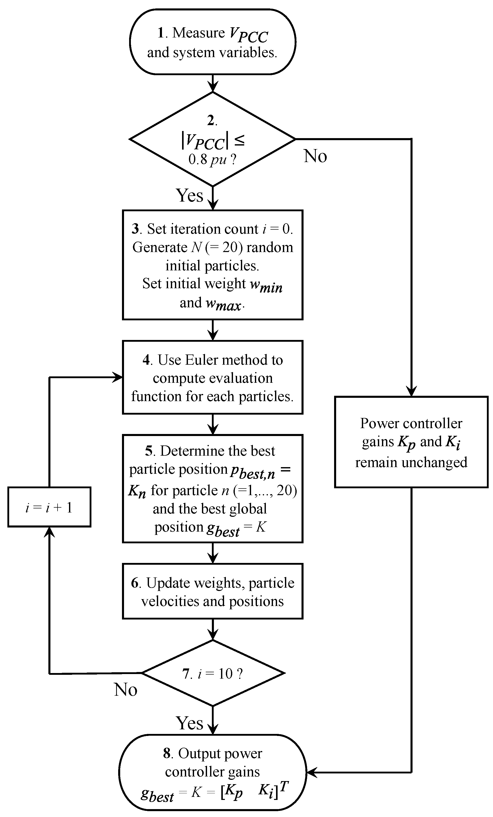
Step (1):

Measure PCC voltage $V_{PCC}$, wind speed $V_w$, rotor speed ${\mathsf{\omega }}_r$, stator currents $i_{ds}$, $i_{qs}$, rotor currents $i_{dr}$, $i_{qr}$, stator voltages $v_{ds}$, $v_{qs}$, rotor voltages $v_{dr}$, $v_{qr}$, stator flux linkages ${\mathsf{\lambda }}_{ds}$, ${\mathsf{\lambda }}_{qs}$, and rotor flux linkages ${\mathsf{\lambda }}_{dr}$, ${\mathsf{\lambda }}_{qr}$ every 0.2 s.

Step (2):

The PSO self-tuning controller is initiated when $\left|V_{PCC}\right| \le 0.8$ pu.

Step (3):

Set initial iteration count i = 0. Generate N (= 20) random initial particles with position vector $K_n^{\left(0\right)}={\left[\begin{array}{cc}{K}_{n,p}^{\left(0\right)}& K_{n,i}^{\left(0\right)}\end{array}\right]}^T$ and velocity vector $V_n^{\left(0\right)}={\left[\mathsf{\Delta }\begin{array}{cc}{K}_{n,p}^{\left(0\right)}& {\mathsf{\Delta }K}_{n,i}^{\left(0\right)}\end{array}\right]}^T$ for particle n (=1,···, 20). Set initial weight $w_n^{\left(0\right)}$=$w_{\max }$= 0.1.

Step (4):

Compute the evaluation function as defined below for each particle.

$$E={\displaystyle \underset{0}{\overset{0.5}{\int }}\left|P_e^{*}-P_e(t)\right|} dt\cong {\displaystyle \sum _{h=1}^{10}\left|P_e^{*}-P_e(t)\right|\Delta t}$$

(23)

where P_e(t) is the predicted real power in the future 0.5 s which can be estimated by the following equation:

$$P_e(t)=-(v_{ds}(t)i_{ds}(t)+v_{qs}(t)i_{qs}(t)+v_{dr}(t)i_{dr}(t)+v_{qr}(t)i_{qr}(t))$$

(24)

A subroutine based on Euler method is developed to estimate the voltages and currents in Equation (24) in the future 0.5 s.

In order to make real power $P_e\left(t\right)$ as close to the desired value $P_e^{*}$ as possible, the evaluation function is selected as the integral of $\left|P_e^{*}-P_e\left(t\right)\right|$dt in the future 0.5 s, as shown in Equation (23).

Step (5):

The best particle position is updated as $K_n{=K}_n^{\left(i\right)}$ when the evaluation function E for particle n with position $K_n^{\left(i\right)}$ at iteration i is less than that for the best particle position $p_{\mathrm{best},n}{=K}_n$ for particle n. Otherwise, $K_n$ remains unchanged. Let particle m (1 ≤ m ≤ 20) with position $K_m^{\left(i\right)}$ be the one with smallest evaluation function among the 20 particles at the i-th iteration. The best global position, $K$, is updated as ${K=K}_m^{\left(i\right)}$ at the i-th iteration if E($K_m^{\left(i\right)}$) < E($K$). Otherwise, $K$ remains unchanged.

Step (6):

Update weights, particle velocities, and particle positions for the next iteration using the following Equations (25)–(27):

$$w_n^{(i)}=w_{\max }-\frac{w_{\max }-w_{\min }}{M}i$$

(25)

$$V_n^{(i+1)}=w_n^{(i)}{V}_n^{(i)}+r_1(K_n-K_n^{(i)})+r_2(K-K_n^{(i)})$$

(26)

$$K_n^{(i+1)}=K_n^{(i)}+V_n^{(i+1)}$$

(27)

where $w_{\max }$ = 0.1, $w_{\min }$ = 0.01, $M$ = 10, and $r_1$ and $r_2$ are random numbers between 0 and 1.

Step (7) and (8):

The PSO algorithm is repeated for M (= 10) iterations in order to reach the desired optimal power controller gains $g_{best}=K={\left[\begin{array}{cc}{K}_p& K_i\end{array}\right]}^T$.

5. Simulation Results

To demonstrate the effectiveness of the proposed PSO self-tuning real power, the dashed position of the system in Figure 1 was simulated using MATLAB/SIMULINK. The parameters for the DFIG are given in the Nomenclature. The simulated dynamic responses of the wind farm subject to a three-phase fault at point “Fault” in Figure 1 are presented as follows. As the settling time reduces with increasing integral gain $K_i$, the gain $K_i$ for the fixed-gain PI controller in Table 1 was tripled in the simulations in order to reduce the simulation time.

5.1. Dynamic Responses for a Fault Voltage of 0.5 pu

Figure 9 compares the dynamic response curves by using MPPT operation mode and by using the proposed de-loaded power control method with fixed-gain PI controller when the wind farm is subject to a three-phase fault at the PCC causing a voltage drop from 1 pu to 0.5 pu.

Based on the response curves in Figure 9, the following observations are in order:

(1)

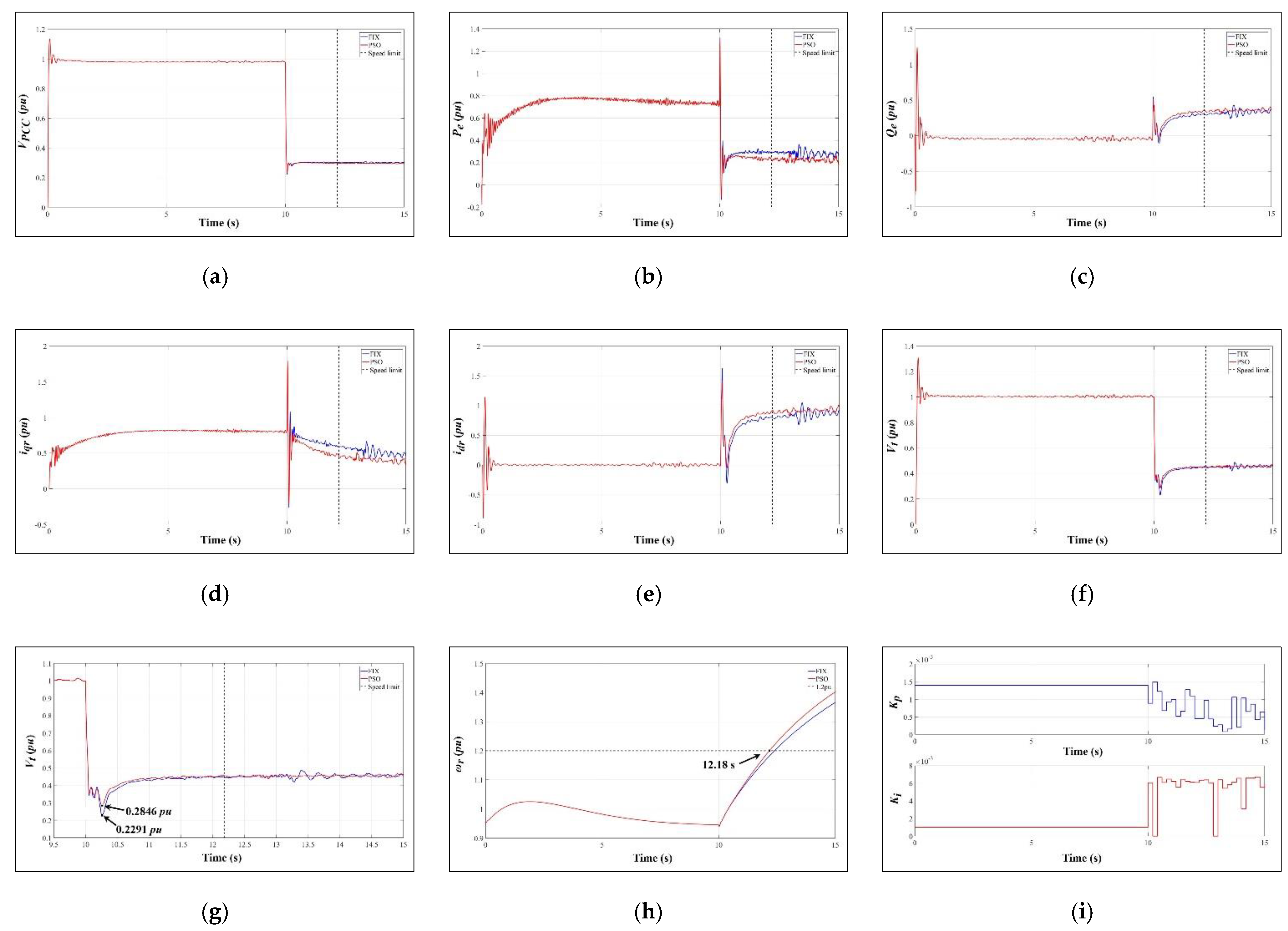
When a low voltage due to a fault is detected at t = 10 s, the real power in Figure 9b for the de-loaded control method with fixed-gain PI controller is reduced by 50% according to Equation (5) through the reduction in q-axis rotor current $i_{qr}$ as shown in Figure 9d. According to Equation (7), the d-axis rotor current $i_{dr}$ in Figure 9e can be increased as a result of the decrease in $i_{qr}$. Thus, the reactive power in Figure 9c is increased and the wind farm terminal voltage in Figure 9f is improved.

(2)

To compare wind farm terminal voltages from the proposed fixed-gain PI de-loaded controller and MPPT operation mode, the dynamic voltage response curves in Figure 9f are enlarged and depicted in Figure 9g. It is observed from Figure 9g that the lowest voltage from the MPPT operation mode is 0.3044 pu while that from the fixed-gain PI de-loaded controller is 0.4083 pu. The lowest voltage is improved by 34.13% when MPPT operation mode is replaced by the fixed-gain de-loaded controller during the faulted period.

Figure 10 compares the dynamic response curves of the wind farm with fixed-gain PI de-loaded controller and PSO self-tuning controller when the grid is subject to a fault of 0.5 pu. Based on the response curves in Figure 10, the following observations can be made:

(1)

To compare the wind farm terminal voltages from the proposed fixed-gain PI de-loaded controller and PSO controller in Figure 4, the dynamic voltage response curves in Figure 10f are enlarged and depicted in Figure 10g. It is observed from Figure 10g that the lowest voltage from the fixed-gain PI controller is 0.4083 pu while that from the PSO controller is improved to 0.4759 pu. A 16% improvement in the lowest voltage can be achieved by the proposed PSO controller than the fixed-gain PI controller.

(2)

The PSO self-tuning controller can yield a better voltage response than the fixed-gain PI controller since its gains $K_p$ and $K_i$ are updated in real time every 0.2 s based on on-line measurements, as shown in Figure 10i.

As the real power output is decreased in the proposed de-loaded power controller in Figure 4 in order to increase the reactive power output and to improve wind farm terminal voltage, generator speed increases during the faulted period. It is thus essential to ensure that the wind farm meets the LVRT requirement set by the local utility (Taiwan Power Company) as depicted in Figure 11.

It is observed from Figure 10h that the generator exceeds the speed limit of 1.2 pu at t = 13.63 s and t = 13.13 s, respectively, for the proposed fixed-gain PI controller and PSO self-tuning controller. This means that the wind farm will remain in a stable operation for a period of 3.63 s and 3.13 s for the fixed-gain controller and self-tuning PI controller, respectively.

Since the required operation time for a fault voltage level of 0.5 pu in Figure 11 is 1.733 s, it is concluded that both the proposed fixed-gain PI controller and the proposed PSO self-tuning controller meet the LVRT requirement.

5.2. Dynamic Responses for a Fault Voltage of 0.3 pu

To examine the effectiveness of the proposed fixed-gain PI controller and PSO self-tuning controller under very low grid voltage, the dynamic responses for the wind farm subject to a 0.3 pu fault voltage at PCC were simulated using MATLAB/SIMULINK and the results are illustrated in Figure 12.

It is observed from Figure 12g that the lowest voltage from the fixed-gain PI controller is 0.2291 pu while that from the PSO controller is improved to 0.2846 pu. A 24.23% improvement in the lowest voltage has been achieved by the proposed PSO controller than the fixed-gain PI controller.

It is also observed from Figure 12h that the durations for the generator to run within the speed limit of 1.2 pu are 2.4 s and 2.18 s for the wind farm with fixed-gain PI controller and PSO self-tuning controller, respectively. Since the minimal operation time is 1.1 s from Figure 11, both controllers meet the LVRT requirement.

6. Conclusions

To improve the wind farm terminal voltage and to provide reactive power support to the system under grid fault situations, a de-loaded real power control strategy implemented with both a fixed-gain PI controller and a PSO self-tuning controller has been proposed. The effectiveness of the proposed de-loaded real power control strategy has been demonstrated on an offshore wind farm in Taiwan using MATLAB/SIMULINK simulations. Specific conclusions are as follows:

(1)

When the wind farm is subject to a grid fault, the wind farm terminal voltage drops to a very low level if the wind farm remains in MPPT operation mode. The terminal voltage can be improved if the wind farm is operated using the proposed real power de-loaded control strategy with a fixed-gain PI controller. The reactive power output of the wind farm can also be increased. Further improvement in voltage profile can be achieved if the fixed-gain PI controller is replaced by the proposed PSO self-tuning controller.

(2)

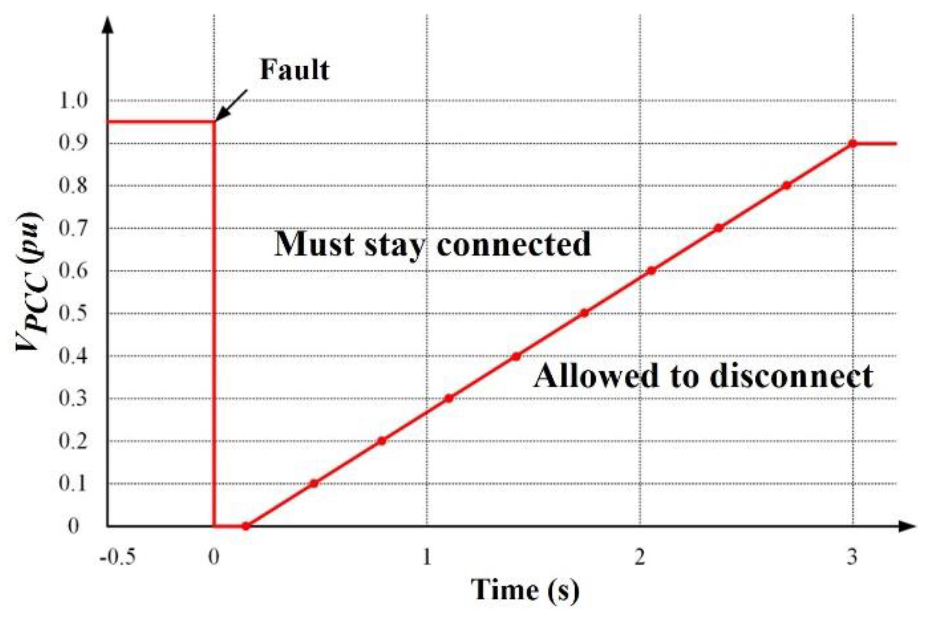
Since the improvement in voltage profile is achieved by increasing reactive power output and decreasing real power output, generator speed will increase at a higher rate than that in the MPPT operation mode. In addition, the de-loaded strategy with a PSO self-tuning controller, which gives a better voltage profile than that with a fixed-gain PI controller, has a higher rate of increase in generator speed and a shorter duration for the generator to operate within the speed limit of 1.2 pu. However, the LVRT requirement is met by both the fixed gain and PSO controllers.

(3)

Future works will be devoted to the coordination of pitch angle controller and de-loaded strategy in order to improve the voltage profile and duration of stable operation further.

(4)

Only the design of the rotor side converter is investigated in this work. Proper design of the grid side converter may help improve the voltage profile.

(5)

Only LVRT is studied in this work. The high-voltage ride through (HVRT) will be investigated in future works.

References

- Liu, W.; Wu, Y.; Lee, C.; Chen, C. Effect of low-voltage-ride-through technologies on the first Taiwan offshore wind farm planning. IEEE Trans. Sustain. Energy 2011, 2, 78–86. [Google Scholar] [CrossRef]
- López, J.; Sanchis, P.; Roboam, X.; Marroyo, L. Dynamic behavior of the doubly fed induction generator during three-phase voltage dips. IEEE Trans. Energy Convers. 2007, 22, 709–717. [Google Scholar] [CrossRef]
- López, J.; GubÍa, E.; Sanchis, P.; Roboam, X.; Marroyo, L. Wind turbines based on doubly fed induction generator under asymmetrical voltage dips. IEEE Trans. Energy Convers. 2008, 23, 321–330. [Google Scholar] [CrossRef]
- Marques, G.D.; Sousa, D.M. Understanding the doubly fed induction generator during voltage dips. IEEE Trans. Energy Convers. 2012, 27, 421–431. [Google Scholar] [CrossRef]
- Pannell, G.; Atkinson, D.J.; Zahawi, B. Minimum-threshold crowbar for a fault-ride-through grid-code-compliant DFIG wind turbine. IEEE Trans. Energy Convers. 2010, 25, 750–759. [Google Scholar] [CrossRef]
- López, J.; GubÍa, E.; Olea, E.; Ruiz, J.; Marroyo, L. Ride through of wind turbines with doubly fed induction generator under symmetrical voltage dips. IEEE Trans. Ind. Electron. 2009, 56, 4246–4254. [Google Scholar] [CrossRef]
- Pannell, G.; Zahawi, B.; Atkinson, D.J.; Missailidis, P. Evaluation of the performance of a DC-link brake chopper as a DFIG low-voltage fault-ride-through device. IEEE Trans. Energy Convers. 2013, 28, 535–542. [Google Scholar] [CrossRef]
- Yang, J.; Fletcher, J.E.; O’Reilly, J. A series-dynamic-resistor-based converter protection scheme for doubly-fed induction generator during various fault conditions. IEEE Trans. Energy Convers. 2010, 25, 422–432. [Google Scholar] [CrossRef] [Green Version]
- Zhang, S.; Tseng, K.; Choi, S.S.; Nguyen, T.D.; Yao, D.L. Advanced control of series voltage compensation to enhance wind turbine ride through. IEEE Trans. Power Electron. 2012, 27, 763–772. [Google Scholar] [CrossRef]
- Okedu, K.E.; Muyeen, S.M.; Takahashi, R.; Tamura, J. Wind farms fault ride through using DFIG with new protection scheme. IEEE Trans. Sustain. Energy 2012, 3, 242–254. [Google Scholar] [CrossRef] [Green Version]
- Yan, X.; Venkataramanan, G.; Wang, Y.; Dong, Q.; Zhang, B. Grid-fault tolerant operation of a DFIG wind turbine generator using a passive resistance network. IEEE Trans. Power Electron. 2011, 26, 2896–2905. [Google Scholar] [CrossRef]
- Yan, X.; Venkataramanan, G.; Flannery, P.S.; Wang, Y.; Dong, Q.; Zhang, B. Voltage-sag tolerance of DFIG wind turbine with a series grid side passive-impedance network. IEEE Trans. Energy Convers. 2010, 25, 1048–1056. [Google Scholar] [CrossRef]
- Huang, P.; Moursi, M.S.E.; Hasen, S.A. Novel fault ride-through scheme and control strategy for doubly fed induction generator-based wind turbine. IEEE Trans. Energy Convers. 2015, 30, 635–645. [Google Scholar] [CrossRef]
- Ibrahim, A.O.; Nguyen, T.H.; Lee, D.; Kim, S. A fault ride-through technique of DFIG wind turbine systems using dynamic voltage restorers. IEEE Trans. Energy Convers. 2011, 26, 871–882. [Google Scholar] [CrossRef]
- Wessels, C.; Gebhardt, F.; Fuchs, F.W. Fault ride-through of a DFIG wind turbine using a dynamic voltage restorer during symmetrical and asymmetrical grid faults. IEEE Trans. Power Electron. 2011, 26, 807–815. [Google Scholar] [CrossRef] [Green Version]
- Abdel-Baqi, O.; Nasiri, A. Series voltage compensation for DFIG wind turbine low-voltage ride-through solution. IEEE Trans. Energy Convers. 2011, 26, 272–280. [Google Scholar] [CrossRef]
- Amalorpavaraj, R.A.J.; Kaliannan, P.; Padmanaban, S.; Subramaniam, U.; Ramachandaramurthy, V.K. Improved fault ride through capability in DFIG based wind turbines using dynamic voltage restorer with combined feed-forward and feed-back control. IEEE Access 2017, 5, 20494–20503. [Google Scholar] [CrossRef]
- Ambati, B.; Kanjiya, P.; Khadkikar, V. A low component count series voltage compensation scheme for DFIG WTs to enhance fault ride-through capability. IEEE Trans. Energy Convers. 2015, 30, 208–217. [Google Scholar] [CrossRef]
- Kanjiya, P.; Ambati, B.B.; Khadkikar, V. A novel fault-tolerant DFIG-based wind energy conversion system for seamless operation during grid faults. IEEE Trans. Power Syst. 2014, 29, 1296–1305. [Google Scholar] [CrossRef]
- Flannery, P.; Venkataramanan, G. Unbalanced voltage sag ride-through of a doubly fed induction generator wind turbine with series grid side converter. In Proceedings of the 2008 IEEE Industry Applications Annual Meeting, Edmonton, AB, Canada, 5–9 October 2008; pp. 1–8. [Google Scholar] [CrossRef]
- Flannery, P.S.; Venkataramanan, G. A fault tolerant doubly fed induction generator wind turbine using a parallel grid side rectifier and series grid side converter. IEEE Trans. Power Electron. 2008, 23, 1126–1135. [Google Scholar] [CrossRef]
- Zhu, R.; Chen, Z.; Wu, X.; Deng, F. Virtual damping flux-based LVRT control for DFIG-based wind turbine. IEEE Trans. Energy Convers. 2015, 30, 714–725. [Google Scholar] [CrossRef]
- Yang, L.; Xu, Z.; Ostergaard, J.; Dong, Z.Y.; Wong, K.P. Advanced control strategy of DFIG wind turbines for power system fault ride through. IEEE Trans. Power Syst. 2012, 27, 713–722. [Google Scholar] [CrossRef] [Green Version]
- Mokryani, G.; Siano, P.; Piccolo, A.; Chen, Z. Improving fault ride- through capability of variable speed wind turbines in distribution networks. IEEE Syst. J. 2013, 7, 713–722. [Google Scholar] [CrossRef]
- Vieira, J.P.A.; Nunes, M.V.A.; Bezerra, U.H.; do Nascimento, A.C. Designing optimal controllers for doubly fed induction generators using a genetic algorithm. IET Gener. Transm. Distrib. 2009, 3, 472–484. [Google Scholar] [CrossRef]
- Kennedy, J.; Eberhart, R. Particle swarm optimization. In Proceedings of the ICNN’95-International Conference on Neural Networks, Perth, WA, Australia, 27 November–1 December 1995; Volume 1944, pp. 1942–1948. [Google Scholar]
- Kennedy, J.; Eberhart, R. A new optimizer using particle swarm theory. In Proceedings of the MHS’95 Sixth International Symposium on Micro Machine and Human Science, Nagoya, Japan, 4–6 October 1995; pp. 39–43. [Google Scholar]
- Yang, J.S.; Chen, Y.W.; Hsu, Y.Y. Small-signal stability analysis and PSO self-tuning frequency control for an islanding system with DFIG wind farm. IET Gener. Transm. Distrib. 2019, 13, 563–574. [Google Scholar] [CrossRef]
- Pena, R.; Clare, J.C.; Asher, G.M. Doubly fed induction generator using back-to-back PWM converters and its application to variable-speed wind-energy generation. IEE Proc. Electr. Power Appl. 1996, 143, 231–241. [Google Scholar] [CrossRef] [Green Version]
- Weng, Y.T.; Hsu, Y.Y. Sliding mode regulator for maximum power tracking and copper loss minimisation of a doubly fed induction generator. IET Renew. Power Gener. 2015, 9, 297–305. [Google Scholar] [CrossRef]