Comparison of Energy Prediction Algorithms for Differential and Skid-Steer Drive Mobile Robots on Different Ground Surfaces

Abstract

A detailed literature analysis depicts that artificial neural networks are rarely used for the power consumption estimation in the mobile robotics field. Instead, researchers prefer to develop analytical models of investigated robots. This manuscript presents a comparison of mathematical models and non-complex artificial neural networks in energy prediction tasks for differential and skid-steer drive robots which move over various types of surfaces. The results show that both methods could be used interchangeably but AI methods are more universal, do not depend on the kinematic structure of a robot and are tolerant for designers not having a complex knowledge about the system.

1. Introduction

The objective of energy prediction algorithms is to answer the question about how long a device will stay operational when it is supplied by a power source with a limited amount of energy. Especially in the field of robotics, such knowledge allows to use system management methods to design robust robots (by assuring uninterrupted access to energy during execution of the mission) with implemented optimization methods providing reduction of power consumption [1,2]. As a result, mobile robots can operate longer [3] and the path planners can significantly increase the energy efficiency in comparison to the classical ones based on path length minimalization [4].

In the industrial environment, the most popular robots are differential and skid-steer drive mobile robots; thus, the research introduced in this article focuses on the mentioned types. It is common in energy prediction algorithm development, that researchers, based on an analytical description of robot–ground interaction, create mathematical models of the robots and identify their coefficients as a result of experiments. Creation of models independent of robot’s kinematic structure requires an experimental identification of many parameters [5], such as motor’s coefficients which can be unavailable for the main robot’s computer making the process of automatic calibration almost impossible. Usually, designers of algorithms create a mathematical description of the power consumed during robot’s movement only for a specific drive type because the influence of lateral friction forces acting on skid-steer robots during driving are not negligible [6,7,8].

Therefore, the differential drive models [1,9,10] cannot be used directly for power estimation of skid-steer drive. However, robots for low velocities, not higher than human walking speed [11], can be treated as differential with wheels located in instantaneous centers of rotation (ICR) of the left and right side of the robot’s body [12]. This method simplified the description of skid-steer robots and was used in an energy prediction algorithm [13,14] which is valid for any skid-steer suspension, such as 4-wheels, 6-wheels or tracks [6,15].

The main drawback of abovementioned methods is the necessity of finding an analytical formula describing the system behavior. This can be extremely difficult for complex robotic constructions. To deal with the problem, the mathematical model could be replaced by an artificial neural network as a nonlinear approximation. After the literature review, it seems that the AI techniques are rarely used for power consumption estimation. In [16], it is shown that the usage of feedforward and recurrent neural networks trained offline can be used to find the battery remaining state of a charge based on mission parameters. Another utilization of neural networks is presented in [17] to find out how many mission steps can be completed before the robot’s battery will be fully discharged. In both articles, the authors used precisely known battery data, therefore, the methods cannot be directly used to determine the robot’s energy demand when it is supplied by another power source. The low popularity of the neural network usage in the described field indicates a gap which should be filled by a detailed investigation.

The aim of our research is to use energy prediction algorithms which require as few as possible robotic sensors to provide universality for a wide range of robots. Therefore, there is no exteroceptive sensor used, the presented methods are based on the robot velocity and surface parameters. For calibration purposes, only proprioceptive sensors are used, capable to measure:

• The battery’s power consumption;
• The angular velocity of the wheels;
• The angular velocity of the robot.

The comparative analysis was used to check whether the performance of AI algorithms is good enough for being used as replacement for more complex analytical approaches and determine the sense of deeper research.

The paper is organized as follows. Section 2 introduces the theoretical background explaining the principles of algorithms operation. Section 3 describes the testing setup with an overview of hardware and software used. Section 4 shows the results of mathematical model-based energy prediction algorithms for differential and skid-steer drive robots, the performance of an alternative method of artificial neural network usage, and the comparative analysis. At the end, Section 5 contains the results discussion and Section 6 includes conclusions and proposes future development directions.

2. Background

2.1. Division of Power Consumed by Robots

In mobile robots, the battery energy consumption can be divided into three factors [1]:

• Motion system—the power depends on motion dynamics and robot-ground interactions;
• Sensing system—the power depends on frequency of used sensors;
• Control system—the power consumed by computers and microcontrollers is approximately constant.

When sensors work with an invariant frequency, the power of the sensing system can also be treated as a constant [9], and the total robot power $P_d$ can be formulated as:

$$P_d=P_L+P_m$$

(1)

where $P_m$ is the motion power and $P_L$ is the logical power (sum of sensing and control powers).

The $P_m$ factor is a complex function of the robot’s motion and is described in details in the following sections.

2.2. Mathematical Model of Differential Drive Robot

The scheme of a differential drive mobile robot is shown in Figure 1.

The following description refers to the energy model from the chapter related to modeling in [9].

The power $P_m$ can be written as a sum of kinetic power $P_k$ and friction power $P_f$:

$$P_k\left(t\right)=mv\left(t\right)a\left(t\right)+I{\omega }_z\left(t\right)\beta \left(t\right)$$

(2)

where $m$ denotes the robot mass, $I$ the robot moment of inertia, $v$ and ${\omega }_z$ denote the linear and angular velocities, while $a$ and $\beta$ denote the linear and angular accelerations, respectively.

$$P_f\left(t\right)=\frac{2f_{\mu }}{r} v\left(t\right)+T$$

(3)

where $f_{\mu }$ (Nm) denotes the friction coefficient between wheels and the surface, $r$ denotes the wheel radius, and $T$ (W) denotes the power necessary to overcome the static friction.

The total power $P_d$ of the differential drive robot is equal to:

$$P_d\left(t\right)=P_L+mv\left(t\right)a\left(t\right)+I{\omega }_z\left(t\right)\beta \left(t\right)+\frac{2f_{\mu }}{r}v\left(t\right)+T$$

(4)

When the robot stays motionless, Equation (4) can be written as

$$P_d\left(t\right)=P_L$$

(5)

This allows to find experimentally the power consumed by the logical subsystem.

For a robot moving with the constant, non-zero linear velocity and zero angular velocity, Equation (4) can be written as

$$P_d\left(t\right)-P_L=\frac{2f_{\mu }}{r}v\left(t\right)+T$$

(6)

Using the linear approximation algorithms, the other parameters, i.e., $f_{\mu }$ and $T$ could be found.

2.3. Mathematical Model of Skid-Steer Drive Robot

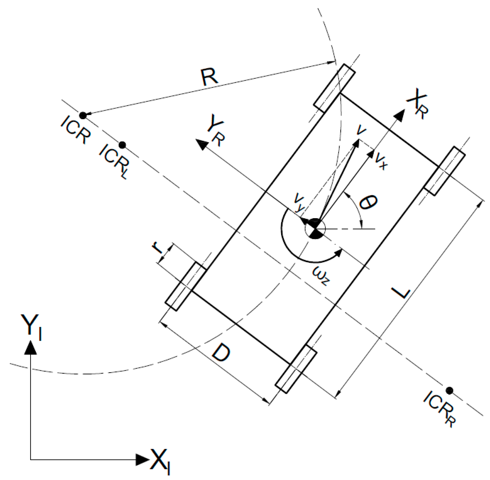
The 4-wheel skid-steer drive mobile robot is shown in Figure 2.

Assume the skid-steer robot is moving with velocity v around the point marked as $ICR$, the curved path radius is equal to R. On the line parallel to the Y_R axis lie instantaneous centers of rotation of the left ($IC{R}_L$) and right ($IC{R}_R$) robot trunk side [18]. The points have following coordinates

$$ICR=\left(x_G, y_G\right)$$

(7)

$$IC{R}_L=\left(x_L, y_L\right)$$

(8)

$$IC{R}_R=\left(x_R, y_R\right)$$

(9)

The robot’s angular velocity related to these points is equal to ${\omega }_z$, so the positions can be determined as

$$x_G=x_L=x_R=-\frac{v_y}{{\mathsf{\omega }}_z}$$

(10)

$$y_G=\frac{v_x}{{\mathsf{\omega }}_z}$$

(11)

$$y_L=\frac{v_x-v_l}{{\mathsf{\omega }}_z}$$

(12)

$$y_R=\frac{v_x-v_r}{{\mathsf{\omega }}_z}$$

(13)

The kinematic dependencies can be established as follows

$$\left[\begin{array}{c}{v}_x\\ v_y\\ {\omega }_z\end{array}\right]=\mathit{A}\left[\begin{array}{c}{v}_l\\ v_r\end{array}\right]$$

(14)

where $\mathit{A}$ is a parameter matrix [12]. Assuming that the wheels have a point contact with a ground, the model is symmetrical, i.e., the distance between robot’s center of gravity (COG) and both $IC{R}_L$ and $IC{R}_R$ are equal, and the COG lies directly in the geometric center point, then, the matrix $\mathit{A}$ can be formulated as

$$\mathit{A}=\frac{1}{2y_0}\left[\begin{array}{cc}{y}_0& y_0\\ 0& 0\\ -1& 1\end{array}\right]$$

(15)

where $y_0$ = $y_L$= −$y_R$.

Then, Equation (14) describes forward kinematics for the differential drive robot where the wheel separation distance is equal to $2y_0$ as shown in Figure 3.

Let us define the steering efficiency coefficient $\chi$ as the inverse of the normalized distance between left and right sides [12]:

$$\chi =\frac{D}{2y_0}, \chi \in \left(0, 1\right]$$

(16)

The maximum value of $\chi$ is equal to 1 what means that no slippage during movement occurs.

Basing on chapter III “Motor power consumption modeling and identification” in [13], the total motion power $P_m$ of the skid-steer robot can be formulated as a sum of slippage power loss $P_s$ and the power loss $P_R$ which is caused by an influence of soil and wheel deformations, the rolling friction and the resistance of mechanical parts of a drive.

$$P_m=P_s+P_R$$

(17)

The approximation of $P_s$ can be written as

$$P_s=\mu |{\mathsf{\omega }}_z|{\displaystyle \sum }_{n=1}^4{p}_{R, L}\left(n\right)\left|{\overline{a}}_{\mathrm{R}, \mathrm{L}}-{\overline{C}}_{\mathrm{R}, \mathrm{L}}\right|$$

(18)

where $\mu$ denotes the friction coefficient, $p\left(n\right)$ denotes the normal force acting on the n-th wheel, $\left|a-C\right|$ denotes the distance between the $ICR$ point and a specific robot wheel as per Figure 4. The R, L subscripts relate to the right and left side of the robot body, respectively.

The approximation of $P_R$ can be formulated as:

$$P_R=G\left(\left|v_l\right|+\left|v_r\right|\right)$$

(19)

where $G$ denotes the proportionality factor, $v_l$ and $v_r$ denote linear velocity of left and right robot side, respectively.

The steering efficiency coefficient $\chi$ can be found by measuring the total robot rotation angle $\phi$ when linear velocities of the left and right robot sides had been opposite [19].

$$\chi =D\phi /\left({{\displaystyle \int }}^{ }{v}_{r}dt-{{\displaystyle \int }}^{ }{v}_{l}dt \right)$$

(20)

where $D$ is the distance between the left and right side wheels.

Using Equation (16), the $y_0$-coordinate can be calculated using the following formula

$$y_0=\frac{D}{2\chi }$$

(21)

The knowledge of $y_0$ determinates the position of $C_L$ and $C_R:$

$$C_L=(0, y_0)$$

(22)

$$C_R=(0,-y_0)$$

(23)

To define the parameters $\mu$ and $G$, the minimum value of the cost function $J\left(\mu , G\right)$ should be found.

$$J\left(\mu , G\right)={\displaystyle \sum }_{\forall t}{\left(P_m\left(t\right)-{\widehat{P}}_m\left(t,\mu , G\right)\right)}^2$$

(24)

where $P_m\left(t\right)$ denotes the real power consumption and ${\widehat{P}}_m\left(t,\mu , G\right)$ denotes the estimated power consumption calculated using Equation (17).

2.4. Artificial Neural Network

As an alternative method, the feedforward neural networks were used to approximate the model of the robot. For learning, validating and testing, a Matlab extension named Deep Learning Toolbox was used. As a performance function during learning, we chose the Mean Squared Error defined as the average squared error between network and target outputs, for the performance function optimalization, we used the Levenberg–Marquardt algorithm, which is one of the fastest methods for small neural networks. Additionally, the learning rate was set to 10⁻⁴ and the learning process was terminated if one of the following assumptions were true:

• The number of epochs exceeded 2000;
• The gradient was lower than 10⁻¹⁵;
• The number of consecutive iterations when the validation error continuously increases exceeded 50;
• The damping factor used in the Levenberg–Marquardt algorithm exceeded 10¹⁰.

The number of inputs depends on the type of robot; for differential drive, the following five inputs were used:

• The linear velocity $v$;
• The angular velocity ${\omega }_z;$
• The $f_{\mu }$ and $T$ coefficients;
• The additional mass.

For the skid-steer drive, there were six inputs:

• The linear velocity $v$;
• The angular velocity ${\omega }_z;$
• The $y_0,$ $\mu$ and $G$ coefficients;
• The additional mass.

Note that for an approximation of the power consumption of the robot moving on a specific type of surface, the coefficients are not necessary but using them allows to create a more versatile neural network which can be used to estimate power during the mission on different types of surfaces.

For both networks, only one hidden layer with 10 neurons was used. As an activation function for the hidden layer, we used radbas and for the output layer—poslin.

The training input data were randomly divided into three subsets as per Deep Learning Toolbox default settings:

• The data used for learning contained 70% of training input data;
• The data used for validation contained 15% of training input data;
• The data used for testing contained 15% of training input data.

Three subsets are required by some of Matlab’s learning termination conditions. Considering a random division of input data for testing purpose, we used a separate test dataset which helps better visualize the quality of the network after offline learning.

3. Test Setup

3.1. The Hardware

In this research, we used a modified TurtleBot3 robot with a different number of wheels and the distances between them. One of the skid-steer robot configurations is shown in Figure 5. A total of four robots have been used and each of them includes the following parts: power supply, microcontroller, drives and main computer.

3.1.1. The Power Supply

The robots were supplied by a lithium-polymer battery with 7 Ah capacity and 812 g weight in a 6SP1 configuration. The total battery voltage range was between 19.2 and 25.2 V.

The battery was connected to the hot swap device LM5066I which has overcurrent and overvoltage protection mechanisms. The maximum operational power is equal to 239 W. The device measures the input current and voltage with an accuracy of 1.75% and 1.25%, respectively, using 12-bit ADC sampling with 1 kHz frequency. To reduce the measurement noise, the measured data are averaged using 16 consecutive samples; thus, the acquisition frequency is about 50 Hz. For communication purposes, the PMBus interface was used.

The output of the LM5066I was connected to the buck–boost converter PI3740 whose maximum power is equal to 140 W. The converter output was configured to deliver 12 V to the system and the efficiency of power transfer was 94%.

3.1.2. The Microcontroller

The OpenCR1.0 board was used as a low-level computer of the robot. It contained the STM32 microcontroller with ARM Cortex-M7 core and IMU ICM-20648 with a 3-axis gyroscope, accelerometer and magnetometer.

The IMU was communicated through SPI with STM32 with 0.8 MHz frequency, the gyroscope worked in the 2000 dps range and the accelerometer’s measurement were in ±2 g range.

The STM32 controlled the drive subsystem using a TTL interface and communicated with the main robot computer through UART.

3.1.3. The Drive

For the differential drive robot, two DC motors XL430-W250 were used with a gear ration equal to 258.5:1, a stall torque 1.4 Nm and a no-load speed of 57 rev/min. Additionally, the motors had integrated encoders with a resolution 4096 pulse/rev, and the microcontroller with an ARM Cortex-M3 core which was responsible for communication with the OpenCR1.0 board and implementing the PID regulators for the wheel angular velocity control.

The drive wheels had a diameter equal to 66 mm, and their linear and angular velocities were limited to 0.22 m/s and 2.84 rad/s, respectively, to provide the torque margin.

3.1.4. The Main Computer

As the main computer of the robot, we used a Raspberry Pi 3 Model B+ with Ubuntu 18.04 OS. The core of the microcomputer based on 64-bit ARM Cortex-A53 working with 1.4 GHz clock frequency. The computer communicates through SSH with the remote PC, controls hot swap device and the OpenCR1.0 board.

3.2. The Software

The software was divided into two parts: the control software responsible for robot steering and data acquisition, and the testing software responsible for collected data postprocessing and energy prediction algorithm usage.

3.2.1. The Control Software

The control software was based on Robot Operating System (ROS) structure which enabled to communicate in a distributed environment. The remote PC created the main core node and was sending the control commands to the robot drive. The Raspberry PI was reading the data from hot swap, encoders and IMU, and was publishing the dataset as ROS topic subscribed by the remote PC.

3.2.2. The Testing Software

The testing software was written as python scripts for preprocessing raw data delivered from ROS environment and the algorithms were implemented in Matlab as described in the previous section.

3.3. The Testing Environment

The energy prediction algorithms were tested on four robots defined by their configuration as per

Table 1. The dimension of tested robots.

Drive Type	Differential	Skid-Steer 1	Skid-Steer 2	Skid-Steer 3
Robot length (mm)	160	160	160	160
Wheel separation (x-axis) L (mm)	-	115	185	245
Wheel separation (y-axis) D (mm)	160
Robot width (mm)	180
Wheel width (mm)	18
Wheel radius (mm)	33
Robot mass (kg)	1.86	2.05	2.08	2.11

.

The robots were moving on five surfaces:

• Gypsum block;
• Linoleum;
• Foam mat;
• Floor panels;
• Rubber door mat.

Each of the surfaces had a dimension of 1.5 × 1.5 m, and they had different hardness and roughness.

4. Results

4.1. The Logic System Power

The logic system power for differential and skid-steer drive robots was calculated basing on the data measured during 5-min intervals for a stationary robot. The output was averaged and the standard deviation of the signal was calculated as an indicator of the signal invariability. The results are shown in

Table 2. The logical power experimental results.

Drive Type	Differential	Skid-Steer
Average power PL (W)	6.03	6.92
Standard deviation (W)	0.16	0.14

.

The acquired data confirm that P_L is approximately constant, the higher value for Skid-steer is related to the demand of supplying logical parts of two more motors in comparison to Differential.

4.2. The Parameters of Differential Drive Robot

To find the f_μ and T parameters, the robot was driving along an approximately 35-cm long straight line, with 9 different constant linear velocities. Each drive delivered an average power value, the coefficients were found by using the linear regression technique. The data collected in the calibration and the parameters calculation process on the Floor panels are shown in Figure 6 and Figure 7 respectively.

The results for all of surfaces are summarized in

Table 3. The calculated coefficients for the differential drive mobile robot.

Surface Type	fμ (Nm)	T (W)
Gypsum block	0.21	1.14
Linoleum	0.17	1.21
Foam mat	0.16	1.35
Floor panels	0.16	1.32
Rubber door mat	0.22	1.13

.

4.3. The Differential Drive Mathematical Model Validation

The mathematical model was tested using data collected by manual robot control on each of the surfaces. To compare the real power consumption and the output of the model, two quality factors were calculated:

• The mean square error (MSE) determining the divergence of signals;
• The relative error δ between the estimated energy and the real energy calculated as an integer of power signals.

The real and the estimated power signals are shown in Figure 8.

The calculated outcomes are shown in

Table 4. The calculated values of quality factors for the mathematical model of the differential drive robot.

Surface Type	MSE (W)	δ (%)
Gypsum block	0.12	1.98
Linoleum	0.13	1.21
Foam mat	0.24	2.11
Floor panels	0.08	0.58
Rubber door mat	0.32	2.43

.

The results confirm that the used algorithm works correctly, the maximum relative error equals to 2.43% for the Rubber door mat surface. Note that this particular surface is characterized by a high roughness and the small passive castor wheel, used in differential drive to provide the static stability, had limited ability to rolling without slippage. The algorithm has the highest quality for hard and smooth surfaces, such as Linoleum and Floor panels.

4.4. The Neural Network Usage for Differential Drive Robot

To assess the quality of neural networks, we used the same data collected for calculations in the previous section. We divided the signals into two subsets: first 60 s as training data and the rest as testing data.

The comparison of the real and estimated power calculated by mathematical model and neural network on the Floor Panels is shown in Figure 9.

The quality of the neural network was validated in the same way as output power signals from the previous section. The results are presented in

Table 5. The calculated values of quality factors for the neural network of the differential drive robot.

Surface Type	MSE (W)	δ (%)
Gypsum block	0.55	4.27
Linoleum	0.17	0.83
Foam mat	0.25	1.20
Floor panels	0.07	0.69
Rubber door mat	0.19	0.56

.

The trained neural network estimates the power as accurate as the mathematical model, the quality depends on a non-deterministic learning process (real training set is chosen randomly from the input data) which can cause a different outcome for each iteration.

4.5. The Parameters of Skid-Steer Drive Robot

The $\chi$ parameter was calculated as per Equation (20), using data collected for different angular velocities. As assumed, the values depended on the surface type but were similar for different velocities (Figure 10). The results are shown in

Table 6. The calculated steering efficiency coefficient $\chi$ for different robot and surface types.

Surface/Drive Type	Skid-Steer 1	Skid-Steer 2	Skid-Steer 3
Gypsum block	0.648	0.423	0.290
Linoleum	0.636	0.431	0.294
Foam mat	0.651	0.424	0.273
Floor panels	0.639	0.430	0.294
Rubber door mat	0.637	0.425	0.260

and are equal to the average values for a specific surface type.

Substituting the values from Table 6 into Equation (21), the y₀ coefficient can be found.

Based on

Table 7. The calculated y₀ coefficient (m) for different robot and surface types.

Surface/Drive Type	Skid-Steer 1	Skid-Steer 2	Skid-Steer 3
Gypsum block	0.123	0.189	0.276
Linoleum	0.126	0.186	0.273
Foam mat	0.123	0.189	0.294
Floor panels	0.125	0.186	0.272
Rubber door mat	0.126	0.188	0.308

, the following conclusions can be drawn:

• Increasing the distance between the front and rear wheels deteriorates steering efficiency what causes the increasing y₀ value;
• The y₀ coefficient is similar for each of tested types of surfaces, maximum standard deviation is approximately equal to 1 cm for the Skid-steer 3 robot. It indicates that the slippage is not significantly different.

To find the μ and G parameters, i.e., to minimize the cost function (24), the fminsearch method of Maltab was used. The input data were collected in the calibration process which included the following robot paths:

• Three squares (~40 cm each side) driven with different velocities in the positive direction;
• Repeated the above combination driven backwards.

To calculate the angular velocities of the wheels, the robot’s open-loop controller used inverse kinematics for the differential drive mobile robot, the classical distance between the left and right wheel was replaced with the previously calculated 2y₀ values. Because there was no feedback signal, the position of the robot was estimated by integrating the linear velocity of the wheels.

The coefficients found in the experiment are presented in

Table 8. The calculated μ and G for different robot and surface types.

Drive Type	Skid-Steer 1		Skid-Steer 2		Skid-Steer 3
Surface/Parameters	μ (-)	G (N)	μ (-)	G (N)	μ (-)	G (N)
Gypsum block	1.55	7.60	1.71	7.64	1.68	7.47
Linoleum	0.53	7.43	0.45	7.92	0.46	8.22
Foam mat	1.90	7.17	1.80	7.76	1.70	7.41
Floor panels	0.66	7.38	0.68	7.47	0.73	7.38
Rubber door mat	1.60	7.35	1.52	7.67	1.43	8.28

.

Based on Table 8, the following conclusions can be drawn:

• The μ and G parameters do not depend on the distance of between front and rear wheels;
• The G coefficient for all of the surfaces is similar what suggests that power loss P_R is approximately the same for all robots;
• The μ parameter determinates the surface type, the least power is consumed when moving on smooth, firm surfaces (Linoleum, Floor panels), more energy is necessary for rough, firm surfaces (Gypsum block, Rubber door mat), the most power is drained from the battery when driving on a soft surface (Foam mat).

4.6. The Skid-Steer Drive Mathematical Model Validation

The mathematical model was tested using data collected by a manual robot control on each of surface. To compare the real power consumption with the output of the model, two quality factors, as per differential drive, were calculated: MSE and δ. The results are gathered in

Table 9. The calculated values of quality factors for the mathematical model of skid-steer drive robots.

Drive Type	Skid-Steer 1		Skid-Steer 2		Skid-Steer 3
Surface/Parameters	MSE (W)	δ (%)	MSE (W)	δ (%)	MSE (W)	δ (%)
Gypsum block	0.29	2.92	0.43	1.79	0.32	0.60
Linoleum	0.29	3.70	0.32	2.65	0.30	2.20
Foam mat	0.32	2.81	0.42	1.04	0.40	0.04
Floor panels	0.36	2.94	0.35	3.07	1.22	3.41
Rubber door mat	0.26	2.75	0.60	1.82	0.40	0.74

.

The used algorithm allows a good estimation of the consumed power, the relative error δ oscillates around 3%. This is a satisfactory outcome considering the set of simplifying assumptions.

4.7. The Neural Network Usage for Skid-Steer Drive Robot

To asses quality of neural networks data collected in Section 4.5, we used the training set and data collected in the previous section as the testing set. The same quality factor was computed for the estimated power signal.

Based on

Table 10. The calculated values of quality factors for neural network of skid-steer drive robots.

Drive Type	Skid-Steer 1		Skid-Steer 2		Skid-Steer 3
Surface/Parameters	MSE (W)	δ (%)	MSE (W)	δ (%)	MSE (W)	δ (%)
Gypsum block	1.25	5.83	1.43	4.75	1.50	5.06
Linoleum	0.23	1.62	3.24	6.48	0.84	4.06
Foam mat	1.32	5.21	1.38	4.95	0.88	3.90
Floor panels	0.70	3.18	0.72	4.21	0.45	2.81
Rubber door mat	0.78	5.46	4.46	9.57	0.98	4.75

, the trained neural network estimates the power worse than the mathematical model, the mean average of relative error results of the analytical model (i.e., the average of all δ values in Table 9 equals 2.17%) is approximately two times lower than the mean average of relative errors presented in Table 10 (4.79%). The neural network performance could be increased using a more diverse training dataset (during the calibration process robot moved in straight lines or rotate in place only).

5. Discussion

Despite the quality factors indicate that mathematical models have a better performance, it is to be noted that finding the appropriate description can be an impossible task to do. Moreover, the introduced models require the robot’s specific parameters, such as the radius of wheel or relative position of each wheel in reference to the center of gravity. However, the analytical parameters could not be stable in a long period of time, some of them depend on surface–suspension interactions which makes it hard to determine them. The good accuracy of the mathematical models can be difficult to keep in real scenarios where environment parameters change dynamically causing the necessity of model calibration. The procedure often interrupts execution of the robot’s task (for example, it can require to perform a calibration path) and can be forbidden in some applications.

By using the neural networks, the designer does not have to possess detailed knowledge about the system, there is only need to gather the data (which is also necessary for the parameter identification in mathematical modeling, of course). Additionally, there exists methods of online training the neural networks what makes the process easy to automatize. Especially this feature could be helpful in robotic application where the type of ground is often changing.

The disadvantage of utilization of artificial neural networks is that they require more computational power, particularly during the training process. Although, today even simple microcomputers are able to handle complicated calculations, for the most of the robotics systems, it could not cause any problem. This is true even if the training procedure can be outsourced and can be done on remote machines.

Considering an insignificant contribution of AI methods usage in the energy prediction task in the mobile robotics field and the fact that such algorithms can be used interchangeably with more complex analytical modelling, it may be noticed that the topic constitutes an interesting field for future development.

For the presented research, we used a simple feedforward neural network with only a one hidden layer and we received satisfactory effects. We believe that it is possible to improve the outcomes, to achieve that, we will investigate available machine learning approaches in more detail.

This article states a solid foundation for the prospective works which include testing the artificial neural network power consumption prediction algorithms in the industrial and the outdoor environment, and also checking the quality for other types of robots such unmanned aerial vehicles.

6. Conclusions

The result of current research indicates that both the mathematical model based and neural network-based algorithms can properly estimate the robot’s power consumption using the dynamic behavior as an input. Therefore, the artificial neural networks can be used as replacement for classical, more complex analytical solutions.

In future research, we will investigate the behavior of machine learning-based energy prediction algorithms using automated guided vehicles in the industrial environment which realize delivery tasks in factories and warehouses. In addition, we plan to investigate the proposed methods for different drone applications in the outdoor environment, especially in agriculture during inspection assignments and more complex crop spraying tasks where the mass of the system is changing dynamically. The extended dataset should broaden the view and enable to utilize more advanced machine learning methods.

References

- Mei, Y.; Lu, Y.-H.; Hu, Y.C.; Lee, C.S. Deployment of mobile robots with energy and timing constraints. IEEE Trans. Robot. 2006, 22, 507–522. [Google Scholar] [CrossRef] [Green Version]
- Pentzer, J.; Reichard, K.; Brennan, S. Energy-based path planning for skid-steer vehicles operating in areas with mixed surface types. In Proceedings of the 2016 American Control Conference, Boston, MA, USA, 6–8 July 2016. [Google Scholar]
- Plonski, P.A.; Tokekar, P.; Isler, V. Energy-Efficient Path Planning for Solar-Powered Mobile Robots; Springer: Berlin/Heidelberg, Germany, 2013; Volume 88, pp. 717–731. [Google Scholar]
- Mei, Y.; Lu, Y.-H.; Lee, C.; Hu, Y.C. Energy-efficient mobile robot exploration. In Proceedings of the International Conference on Robotics and Automation, Orlando, FL, USA, 15–19 May 2006. [Google Scholar]
- Hou, L.; Zhang, L.; Kim, J. Energy modeling and power measurement for mobile robots. Energies 2018, 12, 27. [Google Scholar] [CrossRef] [Green Version]
- Pentzer, J.; Brennan, S.; Reichard, K. On-line estimation of vehicle motion and power model parameters for skid-steer robot energy use prediction. In Proceedings of the 2014 American Control Conference, Portland, OR, USA, 4–6 June 2014. [Google Scholar]
- Shamah, B. Experimental Comparison of Skid Steering Vs. Explicit Steering for a Wheeled Mobile Robot. Master’s Thesis, Carnegie Mellon University, Pittsburgh, PA, USA, March 1999. [Google Scholar]
- Galati, R.; Giannoccaro, N.; Messina, A.; Reina, G. A kinematic approach based on an equivalent track for a skid-steering vehicle. PAMM 2015, 15, 631–632. [Google Scholar] [CrossRef]
- Liu, S.; Sun, D. Modeling and experimental study for minimization of energy consumption of a mobile robot. In Proceedings of the 2012 IEEE/ASME International Conference on Advanced Intelligent Mechatronics (AIM), Kaohsiung, Taiwan, 11–14 July 2012. [Google Scholar] [CrossRef]
- Mei, Y.; Lu, Y.-H.; Hu, Y.; Lee, C. A case study of mobile robot’s energy consumption and conservation techniques. In Proceedings of the ICAR ’05, 12th International Conference on Advanced Robotics, Kaohsiung, Taiwan, 11–14 July 2012. [Google Scholar]
- Morales, J.; Martínez, J.L.; Mandow, A.; Garcia-Cerezo, A.; Pedraza, S. Power consumption modeling of skid-steer tracked mobile robots on rigid terrain. IEEE Trans. Robot. 2009, 25, 1098–1108. [Google Scholar] [CrossRef]
- Mandow, A.; Martinez, J.L.; Morales, J.; Blanco, J.L.; Garcia-Cerezo, A.; Gonzalez, J. Experimental kinematics for wheeled skid-steer mobile robots. In Proceedings of the 2007 IEEE/RSJ International Conference on Intelligent Robots and Systems, San Diego, CA, USA, 29 October–2 November 2007. [Google Scholar]
- Morales, J.; Martínez, J.L.; Mandow, A.; Pequeño-Boter, A.; García-Cerezo, A. Simplified power consumption modeling and identification for wheeled skid-steer robotic vehicles on hard horizontal ground. In Proceedings of the 2010 IEEE/RSJ International Conference on Intelligent Robots and Systems, Taipei, Taiwan, 18–22 October 2010. [Google Scholar]
- Anousaki, G.; Kyriakopoulos, K. A dead-reckoning scheme for skid-steered vehicles in outdoor environments. In Proceedings of the IEEE International Conference on Robotics and Automation, New Orleans, LA, USA, 26 April–1 May 2004. [Google Scholar]
- Pentzer, J.; Brennan, S.; Reichard, K. Model-based Prediction of Skid-steer Robot Kinematics Using Online Estimation of Track Instantaneous Centers of Rotation. J. Field Robot. 2014, 31, 455–476. [Google Scholar] [CrossRef]
- Hamza, A. Predicting Mission Power Requirement for Mobile Robots. Master’s Thesis, University of Southern California, Los Angeles, CA, USA, 2015. [Google Scholar]
- Caballero, L.; Perafan, Á.; Rinaldy, M.; Percybrooks, W. Predicting the energy consumption of a robot in an exploration task using optimized neural networks. Electronics 2021, 10, 920. [Google Scholar] [CrossRef]
- Wong, J.Y.; Chiang, C.F. A general theory for skid steering of tracked vehicles on firm ground. Proc. Inst. Mech. Eng. Part D J. Automob. Eng. 2001, 215, 343–355. [Google Scholar] [CrossRef]
- Martínez, J.L.; Mandow, A.; Morales, J.; Pedraza, S.; García-Cerezo, A. Approximating Kinematics for Tracked Mobile Robots. Int. J. Robot. Res. 2005, 24, 867–878. [Google Scholar] [CrossRef]
Figure 1.
The differential drive mobile robot.
Figure 2.
The 4-wheel skid-steer drive mobile robot.
Figure 3.
The replacement model for symmetrical skid-steer robot.
Figure 4.
Figure 5.
One of the skid-steer robot configurations.
Figure 6.
The data collected in the calibration process on the Floor panels.
Figure 7.
The calculation of parameters on the Floor panels.
Figure 8.
The real and the estimated power signals on the Floor panels.