A Comparative Analysis of the ARIMA and LSTM Predictive Models and Their Effectiveness for Predicting Wind Speed

Abstract

Forecasting wind speed has become one of the most attractive topics to researchers in the field of renewable energy due to its use in generating clean energy, and the capacity for integrating it into the electric grid. There are several methods and models for time series forecasting at the present time. Advancements in deep learning methods characterize the possibility of establishing a more developed multistep prediction model than shallow neural networks (SNNs). However, the accuracy and adequacy of long-term wind speed prediction is not yet well resolved. This study aims to find the most effective predictive model for time series, with less errors and higher accuracy in the predictions, using artificial neural networks (ANNs), recurrent neural networks (RNNs), and long short-term memory (LSTM), which is a special type of RNN model, compared to the common autoregressive integrated moving average (ARIMA). The results are measured by the root mean square error (RMSE) method. The comparison result shows that the LSTM method is more accurate than ARIMA.

1. Introduction

The integration of wind energy into modern energy production systems has recently become a significant issue. Wind energy is the fastest-developing and most promising renewable energy source. However, the chaotic nature of the wind is a large obstacle in the way of using it for energy production. Despite the chaotic structures and uncertainty, there are some predictive methods that have been developed for forwarding predictions. Researchers have developed statistical methods in order to minimize the error in guessing methods used to evaluate time series. In recent years, researchers have been increasingly focused on working on artificial intelligence methods to model the human brain. Today, the widely used wind power estimation tools are based on a combination of physics-based and statistical methods. The LSTM algorithm has attracted much attention for its sufficiency in capturing nonlinear trends and dependencies [1,2]. Wind energy is one of the most common renewable energy sources, and has wide applicability, feasibility, and productivity. However, uncertainty and fluctuations in wind speeds are among the biggest obstacles preventing the further penetration of wind energy into the power grid [3]. Wind speed forecasting is a key factor when estimating the expected power of wind turbines in the short, medium, and long term. Based on the accuracy of these forecasts, the profitability of power plants can be calculated more accurately, and this can be used to determine investment profits, operating costs, and production. The accuracy of the short-term and long-term forecasting of wind energy production is of great importance in terms of balancing electricity production using differential sources [4,5,6]. The forecasting process for a time series is directly affected by the choice of an appropriate model for time series data, as this step directly affects the accuracy of the obtained forecasts, and time series data for different sectors mostly have linear and non-linear characteristics, while sometimes suffering from randomness and disturbances. This means traditional methods are, at times, unable to predict efficiently, which has prompted a number of researchers to think about new, more advanced methods to predict wind speed and its future levels. Among these models is the artificial neural networks model, which is an appropriate way to represent the relationships between variables in a different way from the traditional methods. It is an arithmetic system consisting of a number of interrelated units; it is characterized by its dynamic and balanced nature in processing the data entering it [7]. Long short-term memory networks can be applied to time series forecasting. There are many types of LSTM models that can be used for each specific type of time series forecasting problem, but even the most recent LSTM modifications have their own sequence length limitations, and there is still no architecture available that can actually handle very long times. It is important to evaluate developments in deep learning methods for the multistep time series forecasting problem. Natural language and signals such as voice recognition have been processed using the LSTM networks; however, no studies have evaluated the performance of these in time-series forecasting, especially forward multi-step forecasting. Since LSTM networks have the advantage of dealing with time series, with increasing prediction horizons, it is advisable to check the accuracy of their predictive power [8]. This study focuses on the effectiveness of wind speed prediction using long short-term memory (LSTM), a special type of RNN model, with respect to its performance in reducing error rates compared to the most common method of stationary time modeling, autoregressive integrated moving average (ARIMA). The LSTM method is implemented with deep learning to get more efficient results in prediction for a long period of time, due to its pattern recognition property. The study provides in-depth guidance on the data processing and training of LSTM models for a set of wind speed time series data. The main contribution of this paper is the comparison of the traditional algorithms model (ARIMA) and the deep learning-based algorithms model (LSTM).

2. Literature Review

Wind speed prediction plays a vital role in the planning, managing, and monitoring of smart wind power systems. However, due to the stochastic and intermittent nature of the wind, it is difficult to make satisfactory forecasts [9]. In the past, conventional statistical methods have been employed to forecast time series data and have proven useful in particular problems. However, the time series data are not universally applicable, since they are often full of nonlinearity and irregularity, and more errors can be made. However, in recent decades, methods based on machine learning technologies have been widely used to address the data time series problems, where neural network models come to the fore. The neural network has proven itself well in time series analysis. With the help of neural networks, it is possible to model the nonlinear dependence of the future value of the time series on its past values and on the values of external factors [10]. The ANN and ARIMA models are still suitable for the short-term prediction of wind speed [11]. A trial was conducted to obtain the structure of the autoregressive integrated moving average (ARIMA) model, which will be the most efficient based on the least error, by comparing the real time series and the forecasting [12,13]. The ARIMA model was found to be effective for short-term forecasting [14]. The ARIMA model performs better with linear time series and stationary data than with nonlinear and non-stationary data [15]. A forecasting method based on the autoregressive moving average has been proposed to improve the accuracy of short-term wind speed prediction [16]. Recurrent neural networks (RNNs) are one of the most powerful models for processing sequential data such as time series. However, RNN models have their own shortcomings, as traditional RNN models cannot capture the long-term dependencies in the sequence of input data and cannot deal with the problem of long-term dependencies well. In recent times, a lot of recent research has been devoted to developing algorithms for the deep architecture of the recurrent neural network (RNN) and its variant long short-term memory (LSTM), which has proven to be more accurate than the traditional statistical methods of modeling time series data, with impressive results obtained in many fields [9,17,18]. The LSTM model is relatively new and highly sophisticated in dealing with the time series problem compared to several of the available models [19]. Long-term and short-term memory networks (LSTMs) were developed [20] to address the difficulty in training the long-term dependence problems encountered by simple RNNs [21,22]. The ARIMA model and the LSTM neural network were used to investigate the predictability of vision, and the results show that the LSTM network significantly exceeds ARIMA models in terms of forecast accuracy for this problem [23]. The performance of the multistep electrical load prediction using autoregressive integrated moving average (ARIMA) and long short-term memory (LSTM)-based recurrent neural networks (RNN) models was compared, and the results show that the LSTM model is superior to the ARIMA model [24]. For wind energy prediction, the results show that the performance of LSTM is superior to the traditional deep neural network [25]. To predict bitcoin values, the ARIMA and LSTM models were established for a maximum period of 30 days. The results were compared with the MAPE measurement criterion, and it was observed that the LSTM model produced better results than the ARIMA model [26]. A comparative study of a time series model (ARIMA) and a special type of RNN model (LSTM) was carried out to forecast wind energy [27]. To forecast short-term wind speed, three different models were proposed (ARIMA, LSTM, and multi-variable long short-term memory (MV-LSTM)). The results demonstrate that the prediction performance of the MV-LSTM model is superior to that of the traditional ARIMA method and the single-variable LSTM network [28]. The LSTM model was compared with another model with a recurrent neural network by training them using the same data. The results show that the superior model is LSTM when compared with the MAPE measurement criteria [17]. Comparisons of ARIMA, ARIMAX, and simple LSTM models in the context of the problem of predicting future wind power for a given wind turbine in 48 h showed that the ARIMAX model is able to compete with the simple LSTM models. The ARIMA model is unable to compete with either the ARIMAX model or the LSTM model in terms of accuracy [29].

3. Methodology and Data Source

3.1. Data Source

In this study, the wind speed (km/h) data set for the period from 1 May 2021 to 20 June 2021 for Halifax (https://climate.weather.gc.ca/historical_data/search_historic_data_e.html, accessed on 18 September 2021) was analyzed to identify the characteristics of wind speed at hourly timescales. A wind speed time series, such as that in Figure 1, has characteristics such as time-varying mean and variance, which are typical characteristics of a non-stationary time series. Typical patterns cannot be derived directly from the signal, and the prediction of these types of data requires special care.

3.2. Time Series

Time series analysis is a forecasting and analysis method that is frequently used in business, economics, finance, computing, and science. Estimation is made through the model based on the behavior of time-dependent historical data. We have tried to explain the behavior of the data against time via the trend, seasonal fluctuation, cyclical fluctuation, and random fluctuation.

This shows the general trend of data to increase or decrease over a long period of time. It is divided into linear and nonlinear.

Seasonal variation, or seasonality, refers to the predictable movements in the data that occur in regular cycles. A repeating pattern within each year is known as seasonal variation, although the term is applied more generally to repeating patterns within any fixed period.

3.3. ARIMA

There are different time series methods available today. These estimation methods are autoregressive (AR), moving average (MA), autoregressive moving average (ARMA), and the autoregressive integrated moving average (ARIMA) processes. The specified time series method is known as the Box–Jenkins method. Time series methods have been developed assuming that the series is stationary; stationarity means that the series is free from periodic fluctuations, so before the forecasting model is developed, if the series is not stationary, it should be made stationary. The aim of the method is to obtain suitable models with the least parameters.

3.3.1. Autoregressive Process (AR)

This is based on the linear relationship of the lagged values of the time series and the error term. The general expression of the AR (p) model is as follows:

$$x_t={\varnothing }_1{x}_{t-1}+{\varnothing }_2{x}_{t-2}+\dots +{\varnothing }_p{x}_{t-p}+a_t$$

(1)

3.3.2. Moving Average Process (MA)

The MA(q) method is based on the weighted moving average of error values. In general, the MA(q) model can be represented by the formula

$$x_t={\theta }_0{a}_t-{\theta }_1{a}_{t-1}-{\theta }_2{a}_{t-2}-\dots -{\theta }_q{a}_{t-q}$$

(2)

3.3.3. Autoregressive Moving Average (ARMA) Models

The ARMA (p,q) method is based on the application of AR and MA methods together. According to Paul Karapanagiotidis, the autoregressive moving average (ARMA) model of order is the model [30]:

$$x_t={\varnothing }_1{x}_{t-1}+{\varnothing }_2{x}_{t-2}+\cdots +{\varnothing }_p{x}_{t-p}+{\theta }_0{a}_t-{\theta }_1{a}_{t-1}-{\theta }_2{a}_{t-2}-\cdots -{\theta }_q{a}_{t-q}$$

(3)

3.3.4. Autoregressive Integrated Moving Average (ARIMA) Models

The ARIMA method consists of three main processes: diagnostic control, identification, and estimation. In the first stage, which is called diagnostic control, stationarity control is exerted on the given time series data. A stationary time series is a time series in which statistical properties such as mean, variance and covariance are relative to time. Stationarity is essential when constructing the ARIMA model, which makes estimation useful and highly practical. If the given time series is not stationary, the appropriate degree of difference (d) is applied to make it stationary, and its stationarity is tested again. This process is continued until a stationary series is obtained. (d) is a positive integer and is responsible for the degree of difference. If the difference is assessed (d) times, the integration parameter of the ARIMA model is set to (d). Then, the identification process is performed on the stationary data obtained. With this process, the parameters (p) and (q) of the autoregressive (AR) and moving average (MA) transactions are determined. The ARIMA model has been described as ARIMA (p,d,q) [31].

p: Degree of autoregressive model (AR)

d: Degree of difference

q: Degree of the moving average pattern (MA)

$$x_t={\varnothing }_1{y}_{t-1}+{\varnothing }_2{y}_{t-2}+\cdots +{\varnothing }_p{y}_{t-p}+\delta +a_t-{\theta }_1{a}_{t-1}-{\theta }_2{a}_{t-2}\cdots -{\theta }_q{a}_{t-q}$$

(4)

$x_t,x_{t-1}, x_{t-1}, \dots ,x_{t-p}$ are d-order differerence observations, ${\varnothing }_1,{\varnothing }_2, \dots ,{\varnothing }_p$ are coefficients of the d-order difference observations, $\delta$ is the constant value, $a_t, a_{t-1}, a_{t-2}, \dots , a_{t-q}$ are error values, and ${\theta }_1,{\theta }_2, \dots ,{\theta }_p$ are coefficients for errors [32].

Here, for time t, y_t is the linearized real data, and ε_t represents the error in the moving average. The number of parameters required to be calculated in the general ARIMA (p,d,q) model, which is used in the future estimation of series that do not show seasonal fluctuations, is as much as in ARMA (p,q). In the ARIMA (p,d,q) model, p or q can be zero. In this case, the model is reduced to the AR (d,p) or MA (d,q) model type. Although there are many methods of time series estimation, the ARIMA method is most often used. It is possible that this method can be easily applied to time series that are stationary or made stationary by various statistical techniques.

4. Artificial Neural Networks (ANNs)

Artificial neural networks (ANNs) have emerged as a result of the discovery of the computer, the advancement of technology, the ability to store data regularly, and the ability of computers to think, problem-solve, remember and learn [33]. ANN models are similar to each other. Models consist of an input layer, a hidden layer and an output layer. The number of neurons in the input layer can be n, the number of hidden layers can be n, and there can be n neurons in each hidden layer. The output layer usually contains two neurons (in some networks it can have one, two, three,…, n neurons) and gives a result output. The ANN layer structure is as shown in Figure 2.

There are three processors in the structures of ANNs. Weights—the significance level is determined as a result of the interaction with each input weight. A weight of 0 or a very high value does not mean that the relevant input value is unimportant or important to the network. Sum function—this is used to determine the total value received by neurons. Activation function—the value obtained as a result of calibrating all input values with weights is compressed between 0 and 1 by processing with the activation function. When choosing the activation function, functions that can be derived should be preferred [34]. Figure 3 shows the structure of the ANN.

ANN can be used in problems where mathematical equations cannot be established. The fact that it can work with missing data and make generalizations is one of the advantages of ANN. Although this makes artificial neural networks advantageous over other methods, the disadvantages are that they can only work with numerical data, the uncertainty of the training period, the inexplicable behavior of the network, and the inability to find the most suitable model [35].

5. Deep Learning

The most important feature that makes deep learning different from deep learning ANNs is the high number of hidden layers and neurons, and the neurons in the hidden layer are connected to each other in a complex structure. This difference with ANNs has increased the need for powerful hardware to enable deep learning. The introduction of powerful GPU and CPU (central processing unit) hardware has increased the use of deep learning in complex and large data, and successful results have been obtained. There are different deep learning methods, such as different RNN and LSTM, in the literature.

5.1. Recurrent Neural Network (RNN)

Traditional feed-forward neural networks do not do well with time series data and other sequences or sequential data, because the information does not take into account the time order. Furthermore, the input data are processed independently, and the network architecture does not have built-in memory to remember previous information. Recurrent neural networks (RNNs) are a class of neural network. A network architecture can keep the previous information, because it deals with a variable-length sequence due to the presence of a repeating hidden state; by default, the RNN layer’s output contains one vector for each element. RNNs are typically structured and trained as shown in Figure 4 and Figure 5, respectively.

In a typical feed-forward multilayer neural network, an input vector is fed to neurons at the input layer, which is then multiplied by an activation function to produce an intermediate neuron output. This output then becomes the input for the neuron in the next layer. The net input (denoted input_sumi) for this neuron belonging to the next layer is the connection weight (W) times the output of the previous neuron per bias term, as shown in Equation (5). Then the activation function (denoted by g) is applied to input_sumi to get the neuron output from Equations (6) and (7).

$$input\_su{m}_i=w_i{x}_i+b$$

(5)

$$a_i=g\left(input\_su{m}_i\right)$$

(6)

$$a_i=g\left(w_i{x}_i+b\right)$$

(7)

For each time step t, the activation h_(t) and the output y_t are expressed as follows:

$$h_t+g_1\left(w_{hh}{a}_{t-1}+w_{yx}{x}_t+b_h\right)$$

(8)

and

$$y_t=g_2\left(w_{yh}{h}_t+b_y\right)$$

(9)

where w_hx, w_hh, w_yh, b_h and b_y are coefficients that are shared temporally and $g_1, g_2$ are the activation functions.

Recurrent neural networks suffer from short-term memory as vanishing gradients appear in RNNs due to their nature of being recursive and having deep layers. Since the weights are updated in proportion to the gradient, the vanishing gradient or small value will cause a slight change in the weight value. No change in value in the network means that it does not contribute much to learning. In short, training is useless.

$$w=w+\Delta w$$

(10)

$$\Delta w=n\frac{de}{dw}$$

(11)

where $e={\left(Acual Output-Model Output\right)}^{\wedge }2$

$$if\frac{de}{dw} \ll \ll 1 \Rightarrow \Delta w \ll \ll 1 and w\ll \ll 1 \left(Vanishing\right)$$

$$But if \frac{de}{dw} \gg \gg 1\Rightarrow \Delta w\gg \gg 1 and w\gg \gg 1 \left(Exploding\right)$$

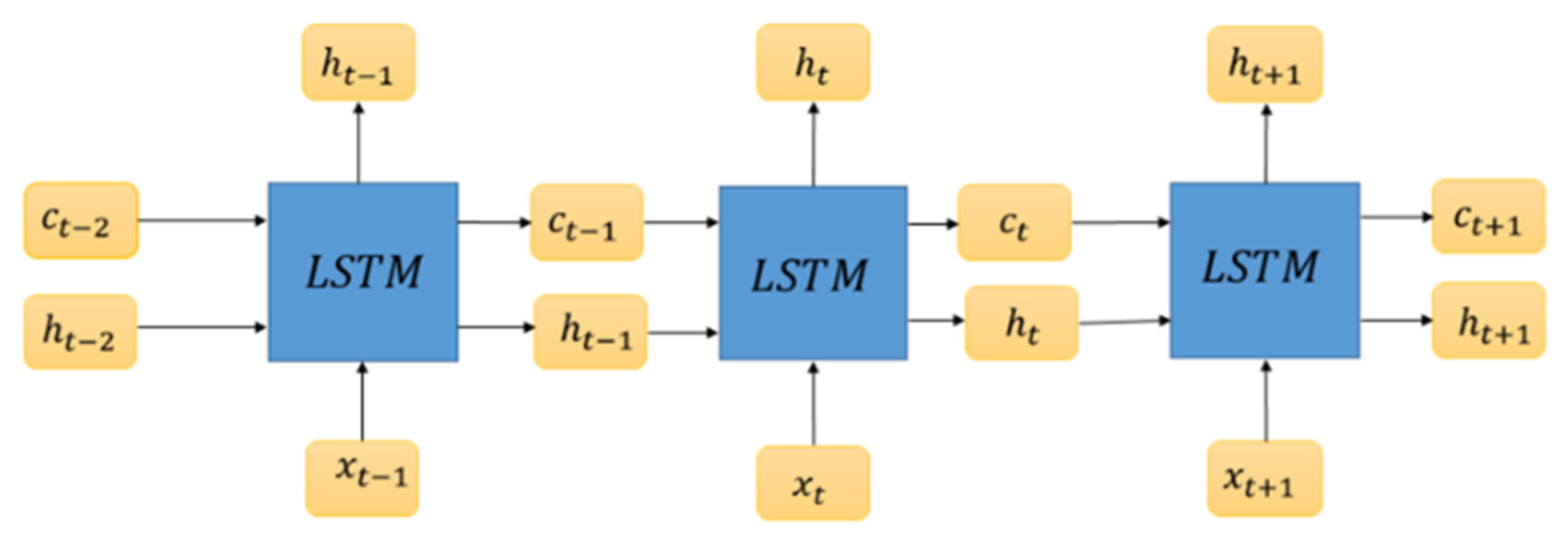
5.2. Long Short-Term Memory (LSTM)

Long short-term memory networks (LSTMs) are very powerful when used in time series prediction problems. LSTMs are explicitly designed to reduce the vanishing and exploding gradient problem during backpropagation in recurrent neural networks. LSTM is generally an RNN, wherein each neuron contains a memory cell that is to able to store past information used by the RNN, or forget it if needed. It has three gates, as follows: the input, to determine the amount of information from the previous layer stored in the cell; the output gate, which determines how the next layer gets to know about the state of the current cell; the forget gate, which determines what to forget about the current state of the memory cell. Figure 6 shows an illustrated graph of LSTM mechanism. LSTM keeps a similar structure to that of standard RNNs, but is different in cell composition. The unique structure of LSTM can effectively solve the problems of gradient disappearance and gradient explosion problems in the training process of RNN. Figure 7 illustrates the schematic diagram of the LSTM network training.

The processing of a time point inside an LSTM cell can be described as below.

The unwanted information in the LSTM is identified and thrown out of the cell state through the sigmoid layer called the forget gate layer.

$$f_f=\sigma \left[w_f\left(h_{t-1},x_t \right)+b_f\right]$$

(12)

where $w_f$ is the weight, $h_{t-1}$ is the output from the previous time stamp, $x_t$ is the new input, and $b_f$ is the bias.

The new information that will be stored in the cell state is determined and updated by the sigmoid layer called the input gate layer. Next, a tanh layer creates a vector of new candidate values that could be added to the state

$$i_t=\sigma \left[w_i\left(h_{t-1}, x_t\right)+b_i\right]$$

(13)

$${\widehat{c}}_i=tanh\left[w_c\left(h_{t-1},x_t\right)+b_i\right]$$

(14)

The old cell state is update, $c_{t-1}$, into the new cell state, $c_t$. The old state is multiplied by $f_t$, forgetting the things that one had decided to forget earlier. Then, $i_t\ast {\widehat{c}}_t$ is added. This gives the new candidate values, scaled by how updated each state value is.

$$c_t=f_t\ast c_{t-1}+i_t\ast {\widehat{c}}_t$$

(15)

A sigmoid layer will be run to decide what parts of the cell state are going to be output. Then, the cell state is put through tanh (to push the values to between −1 and 1) and this is multiplied by the output of the sigmoid gate, so that only the required parts are output.

$$o_t=\sigma \left[w_o\left(h_{t-1},x_t\right)+b_i\right]$$

(16)

$$o_t=\sigma \left[w_o\left(h_{t-1},x_t\right)+b_i\right]$$

(17)

6. Classification of Wind Power Forecasting According to Time-Scales

The time-scale classification of wind power forecasting methods is different in various literature descriptions [36,37].

Table 1. Timescale classifications of wind power forecasting.

Timescale	Range Based on Soman et al. (2010)	Range Based on Foley et al. (2012)
Short term	30 min to 6 h ahead	1–72 h ahead
Medium term	6 h to day ahead	3–7 days ahead
Long term	Day ahead to 1 week or more ahead	Multiple days ahead

shows a summary of the time-scale classification for different forecasting techniques

7. Forecast Validation

To analyze the certainty or accuracy of the models, among the most commonly used parameters for estimating wind velocity predictions are mean absolute error (MAE) and root mean square error (RMSE).

7.1. Root Mean Square Error (RMSE)

Root mean square error (RMSE) is the square root of the mean of the square of all of the error. The use of RMSE is very common in regression, both in statistics and machine learning, and it is considered an excellent general purpose error metric for numerical predictions. A higher RMSE indicates that there are large deviations between the predicted and the actual value. Another important property of the RMSE is that the fact that the errors are squared means that a much larger weight is assigned to larger errors. So, an error of 10 is 100 times worse than an error of 1. RMSE is calculated as:

$$RMSE=\sqrt{\frac{{{\displaystyle \sum }}_{i=1}^N{\left(y_a-y_f\right)}^2}{N}}$$

(18)

where N is the number of errors, y_a is the actual value and y_f is the forecast value. RMSE is a good measure of accuracy, but only to compare prediction errors of different models or model configurations for a particular variable, and not between variables, as it is scale-dependent.

7.2. Mean Absolute Error (MAE)

MAE is simply the mean of the absolute errors. The absolute error is the absolute value of the difference between the forecasted value and the actual value. MAE tells us how big of an error we can expect from the forecast on average. When using the MAE, the error scales linearly. Therefore, an error of 10 is 10 times worse than an error of 1. The RMSE is calculated as:

$$MAE=\frac{1}{N}{\displaystyle \sum }_{i=1}^N\left|y_a-y_f\right|$$

(19)

8. Results

In this study, the hourly data of wind speed in Halifax and the LSTM and ARIMA models are compared.

8.1. ARIMA

For the ARIMA model’s structure selection, the investigation period covers 1 May 2021 to 20 June 2021. From 1224 continuous hourly time series data points of wind speed, we used the first 1200 to build the prediction models. The remaining 24 data points were used for prediction and performance evaluation. To determine the orders, p, and q, the ACF and PACF plots were examined. Figure 8 and Figure 9, respectively, show the ACF and PACF graphs for the wind speed data. In Figure 9, the PACF plot shows that the AR (2) model is suitable for the observed data, because of the cut-off at lag 2.

The series in Figure 1 exhibits repetitive behavior with clearly visible, regularly recurring cycles. This periodic behavior is of interest because the underlying processes of interest can be regular, and the speed or frequency of oscillations that characterize the behavior of the main series will help to identify them. The series shows two main types of fluctuations: obvious sinusoidal waves (bottoms and tops) and a slower frequency that seems to repeat periodically. Typically, non-stationary data cannot be predicted or modeled. The results obtained using non-stationary time series can be false because they can indicate a relationship between two variables where neither of them exists. To obtain consistent and reliable results, non-stationary data must be converted to stationary data. Unlike a non-stationary process, which has variable variance and a mean that does not stay closed, or returns to the long-run average over time, a stationary process returns to a constant long-run mean and has constant variance independent of time. The autocorrelation function (ACF) shows that the values tend to deteriorate slowly, which is an indication of the nonstationary nature of the data, and this transforms it into a stationary series. By taking the first difference of the series analyzed, the plot concludes that the data are stationary, as shown in Figure 10.

After a time series has been stationaryized by differencing, the next step in fitting an ARIMA model is to determine whether AR or MA terms are needed to correct any autocorrelation that remains in differenced series. The analyzed partial autocorrelation and autocorrelation did not give the exact values of the parameters p and q. However, as the studies have shown, the parameter d should be taken as 1, because the values of our time series must be stationary. Figure 11 and Figure 12 show the ACF and PACF for integrated wind speed data. Obviously, integration was needed to make the functions stationary.

To find the best model, the p and q parameters were assigned different values. A new model was built for each pair of parameters. RMSE was chosen to compare the models with each other. The results are shown in

Table 2. RMSE values for different combinations of orders AR (p) and MA (q).

			AR (p)
		0	1	2	3
MA (q)	0	6.6490	4.4601	4.4275	4.4101
	1	4.4149	4.4101	4.2975	4.2912
	2	4.4037	4.4037	4.2904	4.2996

.

From Table 2, it is clear that the best model structure is ARIMA (2,1,2), where the RMSE recorded the lowest value. Using the ARIMA model (2,1,2), wind speed forecasts were made for the next 24 h. Figure 13 shows wind speed actual data and forecast values using ARIMA (2,1,2) model.

8.2. LSTM

In this work, the MATLAB 2019b environment was used to perform the calculations. The LSTM regression network is designed by defining an LSTM-RNN layer with training options. A different initial learning rate was used to find the best training parameter with the lowest RMSE and loss with a learning rate of 0.01. Figure 6 shows the effect of the initial learning rate on the training process. It can be observed that when the learning rate is lower, the training time increases. In this case, you do not derive the best point in the limited repetition, while in a case with a high learning rate, the training time is seen to decrease, and you may experience a gradual increase. If the learning rate is high, the training may not converge at all, or it may even diverge. The degree of change in weight can be large, expanding the improvement beyond the minimum, and this makes the loss function worse. Using a different initial learning rate of 0.01 and time steps tests, we obtained 24, leading to an improvement in the training result and the loss of function falling within an acceptable range. This confirms that the LSTM achieves excellent performance for a long time series data sequence, and the lowest RMSE value is recorded using the given model. Figure 14 illustrates the effect of the initial learning rate on the training process.

During LSTM-RNN training, the forecasted values for the previous step give the feedback of the hidden layer. The model is fitted across all training data, and then the model is updated after each prediction during validation. In this case, the model is fit for an additional two training epochs before making the next forecast. The prediction is canceled using the mean and standard deviation calculated earlier, and then the RMSE is recalculated. Figure 15 shows 24-step forecasting results of wind speed. It is observed that the forecast data of the model in all training epochs are very close to the real data, there are no very sharp fluctuations, resulting in the best overall test RMSE. This means the LSTM algorithm rarely undergoes gradient exploding or a vanishing gradient. Moreover, the predicted results were in a relatively good range, and there would be no significant rising or falling.

Figure 16 shows the Root Mean Square Error (RMSE) of 24-step forecasting for wind speed.

The results of both models were assessed via the RMSE and MAE criterion. According to this measurement result, the LSTM and ARIMA models were compared. From

Table 3. Summary of test statistical errors.

Models	RMSE	MAE
ARIMA	3.423	2.772
LSTM	3.124	2.457

, it is seen that the LSTM model is more efficient than the ARIMA model.

Figure 17 shows a comparison of the hourly data of wind speed in Halifax and the LSTM and ARIMA models. From the figure, we can see that the LSTM model is closer to the actual data, and is more accurate when used in tracking its path compared to the ARIMA model.

9. Conclusions

In this study, the actual data of wind speed were compared with the traditional algorithm (ARIMA) model and the deep learning-based algorithm (LSTM) model. The results show that LSTM is a completely effective technique, as the error rate is lower, so it can be used more frequently for forecasting compared to other models. As we know, LSTM can be implemented with deep learning to get more efficient results in prediction due to its pattern recognition property that functions over a long period of time. As a result of the literature review, it is noted that the ARIMA model produced better results with a smaller quantity of data in previous academic studies. However, the large quantity of data in the models generated within this study shows that deep learning-based algorithms, such as LSTM, outperform traditional algorithms, such as the ARIMA model. It is highly recommended to conduct this study again with more real data, and compare our results with the results of other studies in order to confirm this conclusion.

References

1. Kerem, A.L.; Kirbas, I.; Saygın, A. Performance Analysis of Time Series Forecasting Models for Short Term Wind Speed Prediction. In Proceedings of the International Conference on Engineering and Natural Sciences (ICENS), Sarajevo, Bosnia and Herzegovina, 24–28 May 2016; pp. 2733–2739. [Google Scholar]
2. Kirbas, I.; Kerem, A. Short-term wind speed prediction based on artificial neural network models. Meas. Control. 2016, 49, 183–190. [Google Scholar] [CrossRef]
3. Hanifi, S.; Liu, X.; Lin, Z.; Lotfian, S. A critical review of wind power forecasting methods—Past, present and future. Energies 2020, 13, 3764. [Google Scholar] [CrossRef]
4. Narayana, M.; Putrus, G.; Jovanovic, M.; Leung, P.S. Predictive control of wind turbines by considering wind speed forecasting techniques. In Proceedings of the 2009 44th International Universities Power Engineering Conference (UPEC), Glasgow, UK, 1 September 2009; pp. 1–4. [Google Scholar]
5. National Research Council. Electricity from Renewable Resources: Status, Prospects, and Impediments; National Academies Press: Washington, DC, USA, 2010; pp. 65–73. [Google Scholar]
6. Lydia, M.; Kumar, S.S. A comprehensive overview on wind power forecasting. In Proceedings of the 2010 Conference Proceedings IPEC, Singapore, 27 October 2010; pp. 268–273. [Google Scholar]
7. Lee, D.; Baldick, R. Short-term wind power ensemble prediction based on Gaussian processes and neural networks. IEEE Trans. Smart Grid 2013, 5, 501–510. [Google Scholar] [CrossRef]
8. Chandra, R.; Goyal, S.; Gupta, R. Evaluation of deep learning models for multi-step ahead time series prediction. IEEE Access 2021, 9, 83105–83123. [Google Scholar] [CrossRef]
9. Liu, H.; Mi, X.; Li, Y. Wind speed forecasting method based on deep learning strategy using empirical wavelet transform, long short-term memory neural network and Elman neural network. Energy Convers. Manag. 2018, 156, 498–514. [Google Scholar] [CrossRef]
10. Adebiyi, A.A.; Adewumi, A.O.; Ayo, C.K. Comparison of ARIMA and artificial neural networks models for stock price prediction. J. Appl. Math. 2014, 2014, 614342. [Google Scholar] [CrossRef] [Green Version]
11. Madhiarasan, M. Accurate prediction of different forecast horizons wind speed using a recursive radial basis function neural network. Prot. Control. Mod. Power Syst. 2020, 5, 22. [Google Scholar] [CrossRef]
12. Elsaraiti, M.; Merabet, A.; Al-Durra, A. Time Series Analysis and Forecasting of Wind Speed Data. In Proceedings of the 2019 IEEE Industry Applications Society Annual Meeting, Baltimore, MD, USA, 29 September–3 October 2019; pp. 1–5. [Google Scholar]
13. Grigonytė, E.; Butkevičiūtė, E. Short-term wind speed forecasting using ARIMA model. Energetika 2016, 62, 45–55. [Google Scholar] [CrossRef] [Green Version]
14. Meyler, A.; Kenny, G.; Quinn, T. Forecasting Irish Inflation Using ARIMA Models; Munich Personal RePEc Archive: Munich, Germany, 1998. [Google Scholar]
15. Kam, K.M. Stationary and Non-Stationary Time Series Prediction Using State Space Model and Pattern-Based Approach; The University of Texas at Arlington: Arlington, TX, USA, 2014. [Google Scholar]
16. Tian, Z.; Wang, G.; Ren, Y. Short-term wind speed forecasting based on autoregressive moving average with echo state network compensation. Wind. Eng. 2020, 44, 152–167. [Google Scholar] [CrossRef]
17. Prema, V.; Sarkar, S.; Rao, K.U.; Umesh, A. LSTM based deep learning model for accurate wind speed prediction. ICTACT J. Data Sci. Mach. Learn. 2019, 1, 6–11. [Google Scholar]
18. Greff, K.; Srivastava, R.K.; Koutník, J.; Steunebrink, B.R.; Schmidhuber, J. LSTM: A search space odys-sey. IEEE Trans. Neural Netw. Learn. Syst. 2016, 28, 2222–2232. [Google Scholar] [CrossRef] [Green Version]
19. Goyal, A.; Krishnamurthy, S.; Kulkarni, S.; Kumar, R.; Vartak, M.; Lanham, M.A. A solution to forecast demand using long short-term memory recurrent neural networks for time series forecasting. In Proceedings of the Midwest Decision Sciences Institute Conference, Indianapolis, IN, USA, 12–14 April 2018. [Google Scholar]
20. Schmidhuber, J.; Hochreiter, S. Long short-term memory. Neural Comput. 1997, 9, 1735–1780. [Google Scholar]
21. Hochreiter, S. The vanishing gradient problem during learning recurrent neural nets and problem solutions. Int. J. Uncertain. Fuzziness Knowl.-Based Syst. 1998, 6, 107–116. [Google Scholar] [CrossRef] [Green Version]
22. Bengio, Y.; Simard, P.; Frasconi, P. Learning long-term dependencies with gradient descent is difficult. IEEE Trans. Neural Netw. 1994, 5, 157–166. [Google Scholar] [CrossRef]
23. Salman, A.G.; Heryadi, Y.; Abdurahman, E.; Suparta, W. Weather Forecasting Using Merged Long Short-Term Memory Model (LSTM) and Autoregressive Integrated Moving Average (ARIMA) Model. J. Comput. Sci. 2018, 14, 930–938. [Google Scholar] [CrossRef] [Green Version]
24. Masum, S.; Liu, Y.; Chiverton, J. Multi-step time series forecasting of electric load using machine learning models. In Proceedings of the International conference on artificial intelligence and soft computing, Zakopane, Poland, 3–7 June 2018; pp. 148–159. [Google Scholar]
25. Wu, W.; Chen, K.; Qiao, Y.; Lu, Z. Probabilistic short-term wind power forecasting based on deep neu-ral networks. In Proceedings of the 2016 International Conference on Probabilistic Methods Applied to Power Systems (PMAPS), Beijing, China, 16 October 2016; pp. 1–8. [Google Scholar]
26. Karakoyun, E.S.; Cibikdiken, A.O. Comparison of arima time series model and lstm deep learning algorithm for bitcoin price forecasting. In Proceedings of the The 13th Multidisciplinary Academic Conference, Prague, Czech Republic, 24 May 2018; Volume 2018, pp. 171–180. [Google Scholar]
27. Sandhu, K.S.; Nair, A.R. A comparative study of ARIMA and RNN for short term wind speed forecasting. In Proceedings of the 2019 10th International Conference on Computing, Communication and Networking Technologies (ICCCNT), Kanpur, India, 6 July 2019; pp. 1–7. [Google Scholar]
28. Xie, A.; Yang, H.; Chen, J.; Sheng, L.; Zhang, Q. A Short-Term Wind Speed Forecasting Model Based on a Multi-Variable Long Short-Term Memory Network. Atmosphere 2021, 12, 651. [Google Scholar] [CrossRef]
29. Werngren, S. Comparison of Different Machine Learning Models for Wind Turbine Power Predictions; Uppsala University: Uppsala, Sweden, 2018. [Google Scholar]
30. Karapanagiotidis, P. Dynamic State-Space Models; University of Toronto: Toronto, ON, Canada, 2014. [Google Scholar]
31. Newbold, P. ARIMA model building and the time series analysis approach to forecasting. J. Forecast. 1983, 2, 23–35. [Google Scholar] [CrossRef]
32. Şeyda Çorba, B.; Pelin, K. Wind Speed and Direction Forecasting Using Artificial Neural Networks and Autoregressive Integrated Moving Average Methods. Am. J. Eng. Res. 2018, 7, 240–250. [Google Scholar]
33. Gill, N.S. Artificial Neural Networks Applications and Algorithms. 2019. Available online: https://www.xenonstack.com/blog/artificial-neural-network-applications (accessed on 7 April 2021).
34. Sharma, S.; Sharma, S. Activation functions in neural networks. Towards Data Sci. 2017, 6, 310–316. [Google Scholar]
35. Garver, M.S. Using data mining for customer satisfaction research. Mark. Res. 2002, 14, 8. [Google Scholar]
36. Soman, S.S.; Zareipour, H.; Malik, O.; Mandal, P. A review of wind power and wind speed forecasting methods with different time horizons. In Proceedings of the North American Power Symposium, Arlington, TX, USA, 26 September 2010; pp. 1–8. [Google Scholar]
37. Foley, A.M.; Leahy, P.G.; Marvuglia, A.; McKeogh, E.J. Current methods and advances in forecasting of wind power generation. Renew. Energy 2012, 37, 1–8. [Google Scholar] [CrossRef] [Green Version]
Figure 1. Wind speed time series.
Energies 14 06782 g001
Figure 2. ANN layer structure.
Energies 14 06782 g002
Figure 3. Artificial neural networks structure.
Energies 14 06782 g003
Figure 4. Recurrent neural networks (RNNs).
Energies 14 06782 g004
Figure 5. The training process of RNNs.
Energies 14 06782 g005
Figure 6. LSTM modules including four layers.
Energies 14 06782 g006
Figure 7. The training process of LSTM.
Energies 14 06782 g007
Figure 8. Autocorrelation functions for observed wind speed data.
Energies 14 06782 g008
Figure 9. Partial autocorrelation functions for observed wind speed data.
Energies 14 06782 g009
Figure 10. First difference of wind speed time series.
Energies 14 06782 g010
Figure 11. Autocorrelation functions for integrated wind speed data.
Energies 14 06782 g011
Figure 12. Partial autocorrelation functions for integrated wind speed data.
Energies 14 06782 g012
Figure 13. Forecasts from ARIMA (2,1,2).
Energies 14 06782 g013
Figure 14. Training process with learning rate 0.01 and time step test as 24.
Energies 14 06782 g014
Figure 15. Prediction result with 24 time steps.
Energies 14 06782 g015
Figure 16. RMSE result with 24 time steps.
Energies 14 06782 g016
Figure 17. Twenty-four hours in advance real and forecasted wind speed using ARIMA and LSTM models.
Energies 14 06782 g017