Modelling the Interaction between Air Pollutant Emissions and Their Key Sources in Poland

Abstract

The main purpose of this study is to investigate the relationships between key sources of air pollutant emissions (sources of energy production, factories which are particularly harmful to the environment, the fleets of cars, environmental protection expenditure) and the main environmental air pollution (SO₂, NO_x, CO and PM) in Poland. Models based on MLP neural networks were used as predictive models. Global sensitivity analysis was used to demonstrate the significant impact of individual network input variables on the output variable. To verify the effectiveness of the models created, the actual data were compared with the data obtained through modelling. Projected courses of changes in the variables under study correspond with the real data, which confirms that the proposed models generalize acquired knowledge well. The high MLP network quality parameters of 0.99–0.85 indicate that the network generalizes the acquired knowledge accurately. The sensitivity analysis for NO_x, CO and PM pollutants indicates the significance of all input variables. For SO₂, it showed significance for four of the six variables analysed. The predictions made by the neural models are not very different from the experimental values.

1. Introduction

The World Health Organisation (WHO) considers air pollution the greatest environmental risk factor for human health worldwide [1]. Air pollution is currently perceived as the second biggest environmental concern for Europeans, after climate change [2]. Air contamination is a local, pan-European, and hemispheric problem. Air pollutants released in one country may be transferred in the atmosphere, contributing to or resulting in poor air quality elsewhere. Europeans, more likely to live next to busy roads or industrial regions and so face higher exposure to air pollution. Energy poverty, which is more prevalent in Southern, Central, and Eastern Europe, is a key driver of the combustion of low-quality solid fuels, such as coal and wood, in low-efficiency boilers for domestic heating [3].

The EU’s clean-air policy is based on three main pillars: (1) the Ambient Air-Quality Directives [4,5]; (2) the NEC Directive [6]; and (3) source-specific legislation establishing specific emission and energy efficiency standards for key sources of air pollution [7,8]. Air pollution shows substantial variability both between areas (higher in Southern Europe) and within areas. Spatial variation is mostly related to the presence of local and regional sources [9]. Individuals stand little chance of protecting themselves from air pollution, thus the need for organised actions involving national, regional, and international organisations and authorities [10].

According to EPA EU reports [8] during recent decades, the emission of PM2.5 in Europe decreased slowly by 30% from 1990 to 2014. In the same period, emissions of SO₂ dropped almost seven-fold. In addition, it is East–Central Europe, and Poland in particular that has seen the highest average annual concentrations of PM10 and PM2.5 [11]. It is widely discussed that the population of the developing countries can be exposed to the various noxious gases originating from the combustion of consumed fossil fuels from production, transportation, and power generation due to limited access to clean energy sources [12]. Most countries rely on fossil fuels in their energy systems, no matter how well developed they are [13]. The use of fossil fuels as the main source of energy for most countries has caused several negative environmental impacts, such as global warming and air pollution [14].

Air pollutants mainly come from combustion processes, various technological processes, as well as vehicle traffic [15], the major ones being sulphur oxides (SO_x), nitrogen oxides (NO_x), carbon monoxide (CO) particulate matter (PM), carbon dioxide, volatile organic compounds (VOCs), chlorofluorocarbons and ammonia (NH₃) [16].

1.1. Emissions of Pollutants in Poland

In Poland, the main sources of air pollution are emissions from fuel combustion, mainly from the energy industry and individual households, as well as emissions from transportation. Polish air protection policy is largely reactive—a drop in air pollution emitted by industry and power engineering occurred in response to the EU requirements for these sectors. However, there are no regulations for installations used in households, i.e., solid fuel furnaces, boilers, or fireplaces. Additionally, in the field of transportation, there is a lack of essential legal solutions to limit the old vehicles which are responsible for producing harmful air pollutants. The main problem related to air quality is the fact that Poland is the largest hard coal producer in the EU [17]. The most important energy carrier extracted in Poland in 2019 was hard coal with a 56.2% share. The second-largest carrier in terms of output was lignite, with a share of 15.2% [18]. These are being mined in Upper Silesia, thus making this a large area with enormous concentration of industry and poor long-term air quality [19]. As an example, Figure 1 presents PM2.5 pollution in Poland compared to other EU countries.

Climate change and various health ailments caused by air pollution have become the subject of numerous scientific studies both in Poland and internationally, and the results [21] have pinpointed road transportation and industrial activities to be the two main emission sources responsible for 80% of total NO_x, 90% of total SO₂, 75% of CO, 60% of total suspended particles and 60% of non-methane volatile organic compounds (NMVOCs). The burning of fossil fuel for heating of individual households is mainly responsible for high levels of air pollution in urban areas during winter season [22]. The so-called criteria pollutants: PM, O₃, NO₂ and SO₂, have been recognized as the key ones influencing human health [23]. PM has gained significant attention due to the increasing concerns related to their effects on human health [24]. A large time-scale observation in major Polish cities between 2014–2017 showed a link between an increase in exposure to pollution in the ambient air and an increase in respiratory tract issues requiring hospital treatment and that, in turn, was correlated with PM2.5 and PM10 [25]. Air pollution at ground level, especially PM2.5, is associated with many of adverse health effects. PM2.5 air pollution was estimated to cause approximately 39,800 premature deaths in the population of Poland in 2000 [26]. The city of Katowice in southern Poland faces the worst PM2.5 hazard in the winter months. The highest concentration of this pollutant as well as other PM2.5-related carbonaceous matter, including BaP occurs because of two factors: the location of the city in a highly industrialised area and the dense urban development, and these result in poor natural ventilation. In contrast, urban areas of northern Poland, which is less industrialised and where gas rather than solid fuels are used, do not face this scale of PM2.5 [27]. In the research [28], population growth was found to be the largest driver of energy consumption and air pollutant emissions from 1997–2010. Investments that reduce the production of electricity, which reduces the negative impact on the environment is one of activities [29]. Air emission pollutant prediction has attracted special legislative and scientific attention due to the harmful effects on human health. Statistical model methods for air pollutant emissions are the subject of numerous studies. Statistical models are suitable for the description of the complex site-specific relationship between air pollutants and explanatory variables, and they often make predictions with a higher accuracy than mechanistic models [30]. Brunelli et al. [31] presented a recurrent NN-based forecaster for prediction of daily maximum concentrations of, PM10, SO₂, NO₂, CO and O₃ in the city of Palermo. The related correlation coefficient ranges from 0.72 to 0.97 for each forecasted pollutant, resulting in a slight difference between the forecast and the measured values. A wavelet-based recurrent NN model was proposed by Prakash et al. [32]. He was able to forecast one-step-ahead hourly and daily mean, and daily maximum concentrations of the common ambient pollutants of CO, NO₂, NO, O₂, SO₂ and PM2.5. The results show that a wavelet network, designed appropriately, may be employed successfully for air-quality forecasting. Gocheva-Ilieva et al. [33] used the powerful data-mining technique of classification and regression trees (CART) to build quality nonlinear models of environmental time series. With this approach, they carried out empirical studies of the daily average concentrations of atmospheric PM10 in the cities of Ruse and Pernik, Bulgaria. The results show that CART models fit well with the data and correctly predict about 90% of the measured values of PM10 with respect to the average daily European threshold value. Another study [34] focused on the prediction of hourly levels up to 8 h ahead for several pollutants (NO, NO₂, CO, SO₂ and O₃) and six locations around Bilbao, Spain. The use of these models based on ANNs can provide Bilbao’s air-pollution network designed primarily for diagnosis purposes, with short-term, real-time predicting capabilities. In another study [35], two types of ANN models using the MLP and the radial basis function (RBF) techniques, are employed to forecast hourly PM10 concentrations in urban areas in Cyprus. The Saharan dust episodes are also forecast very accurately with MLP models. This work developed [36] an online air-pollution forecasting system for the Greater Istanbul area. The presented experiments show that quite accurate predictions of air pollutant indicator levels are possible with a simple NN. In a paper [37], the outcomes indicated that researchers mainly focused on the effects of air pollution on human diseases, urban pollution exposure models, and land use regression (LUR) techniques. O₃, NO_x and PM were the most tested contaminants. ANN methods were preferred in studies of O₃ and PM while LUR were more widely used in studies of NO_x. In a research study of Nieto et al. [38], four models based on VARMA, MLP, SVM and ARIMA are constructed for forecasting the PM10 concentration in the city of Oviedo, in Spain. The monthly average pollutants and PM10concentration are used as input data to forecast the monthly average concentration of PM10 from one to seven months ahead. Results showed that the SVM performs better than the other models when forecasting one month ahead as well as for the following months. In the study [39], it was possible to predict average PM2.5 and PM10 concentrations for the next 24 h by developing forecasting models that used MLP with the consideration of k-means clustering findings. It was demonstrated that considering clustering results as input variables improves PM10 and PM2.5 forecasting models for the most polluted station. A neural-network approach was analysed and benchmarked by Ordieres et al. [40]. They compared three different topologies of neural networks to identify their potential uses by analysing their strengths and weaknesses: MLP, Radial Basis Function (RBF) and Square Multi-Layer Perception (SMLP). To compare the results with the ones provided by the neural-network models they built two classical models: a persistence model and a linear regression. The results clearly demonstrated that the neural approach not only outperformed the classical models but also showed fairly similar values among different topologies.

The results [37] show that the ANN method became an increasingly popular means to predict air pollution, and the interaction between different pollutants attracted increasing research attention, with PM + NO_x and PM + O₃ being the main combinations. Furthermore, the results indicate that since 2010, hybrid methods have rapidly joined the mainstream of air-pollution prediction and have been the fastest-developing research method through Markov chain analysis.

1.2. Air Emission Inventory

Due to many years of neglect, Poland faces now serious challenges of air pollution—one of the most serious in the entire European Union. For several years now, national and international programmes have been available on the market to provide financial support for the replacement of coal-fired boilers with modern low-emission boilers, which promises to reduce emissions from this source in the coming years. For years, coal consumption in this sector has been on an upward trend (Figure 2a), while consumption in power plants and CHP plants has gone down (Figure 2b).

It can be assumed that the increase in coal consumption in households is due to the increase in the number of households in Poland from 31.428 million in 1999 to 33.529 million in 2020 [42]. Changes in emissions of the pollutants in question from major sources are shown in Figure 3. In Poland, it is the energy industry that is responsible for SO_x emissions, mainly SO₂ (Figure 3a), accounting for 49%. The main source of SO₂ emissions in the energy industry is the combustion of fuels, mainly coal, in stationary combustion sources which are responsible for 96% of the national SO₂ emissions.

Other sectors account for 27% and the manufacturing and construction sectors for 20% of emissions [43]. The amount of NO_x emissions has decreased by 39% in comparison to 1990. As in the case of SO₂, the changes started with the collapse of heavy industry in the late 1980s and early 1990s. Since the late 1990s, the largest source of NO_x emissions in the country has been the combustion of fuels in road transportation, where emissions have been growing steadily (Figure 3b). This is mainly due to an increase in the number of vehicles by 287% since 1990, which consequently translates into an increase in fuel consumption (including gasoline, diesel oil, LPG and CNG) by 248% [43]. In addition, cars with old-generation engines have a particular impact.

The increase in emissions from road transportation may significantly impede the achievement of the NO_x reduction goals set in Directive 2016/2284 [43]. In 2019, the largest source of CO emissions was fuel combustion in the category of other sectors (which includes small combustion sources such as households, public buildings, business establishments, etc.) (Figure 3c), which are responsible for 61% of national CO emissions. Another significant source of CO emissions is transportation (Figure 3b), which accounts for 25% of national emissions. The main source of particulate matter PM2.5 emissions are sources belonging to the fuel combustion category, which in 2019 generated as much as 84% of the total emissions of this pollutant. The largest share of emissions in this category comes from the area of other sectors (Figure 3c) (49%) and is mainly the result of coal and wood combustion in households. In 2019, the PM2.5 particulate matter decreased by 67% compared to 1990. The main source of PM10 particulate matter emissions in Poland are stationary combustion processes, most of which falls into the category of other sectors—41%. The second-largest source is the industrial processes sector, which is responsible for 16% of emissions. In 2019, PM10 emissions decreased by 70% compared to 1990 [43].

Road transportation in Poland is a significant source of NO_x, CO and PM emissions. Figure 4 presents the number of vehicles older than 15 years, which make up most vehicles in Poland, broken down by age groups, cars and trucks.

2. Materials and Methods

2.1. Data Description

The inventory of emissions to be reported to the UNECE Convention on Long-Range Transboundary Air Pollution (CLRTAP) and to the European Union as defined in Directive (EU) 2016/2284 of the European Parliament and of the Council of 14 December 2016 on the abatement of national emissions of atmospheric pollutants (the so-called “cap-and-trade directive”) and reported for national statistics includes SO₂, NO_x, CO and PM and other emissions. In Poland, these are largely emissions from fuel combustion, which pose a serious threat to human health and life. Therefore, the input data proposed were the main sources of emissions of the pollutants mentioned above, i.e., hard coal consumption in households (HCCH), hard coal consumption in utility power plants and combined heat and power plants (HCCPP), particularly harmful plants (PHP), total number of passenger cars and trucks older than 15 years (C > 15) as well as data that may have a final impact on the air-quality status, i.e., energy from renewable sources (RSE) and environmental protection expenditure (EPE) [18,43,45,46]. The dataset covers the period 2004–2019 and was selected due to data availability.

2.2. The Aim of the Research

The aim of the research was to (i) find correlations and interactions between the groups of explained and explanatory data, as well as (ii) present possible dependencies in the form of models, and (iii) test the models as a practical predictive tool for forecasting air-pollution emissions. It was assumed that artificial MLP networks will be an adequate tool for predicting pollutant emissions with the assumed input and output variables.

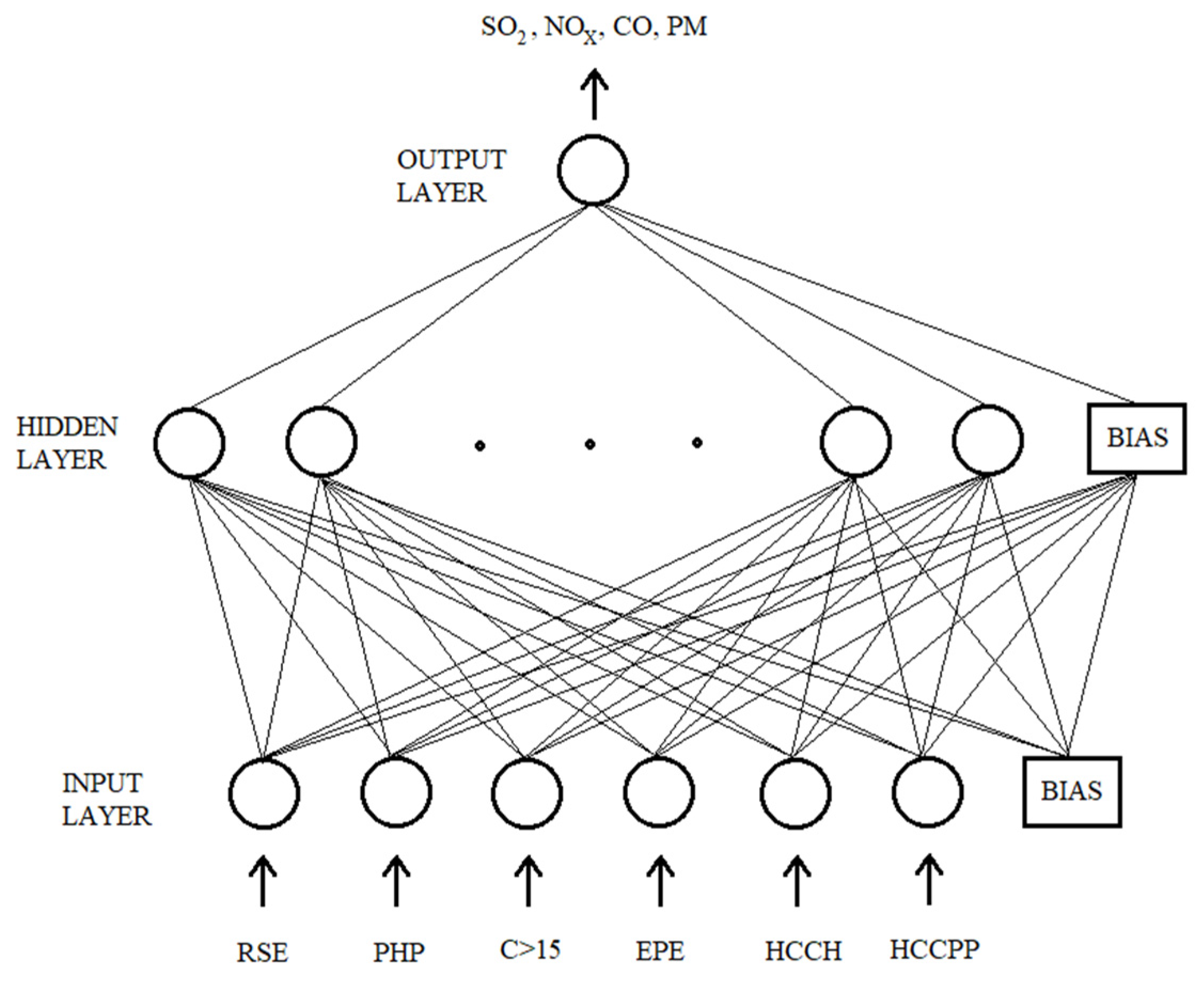
2.3. Description of the Method

The areas of application of neural networks are expanding because they can be successfully used to solve problems requiring data processing and analysis, prediction or classification. One of the many advantages of neural networks is their ability to map very complex, nonlinear relationships between the input and output signals.

Thus, the application of the models in studying pollution proceeds over time or in space, including the degree of influence of various factors or groups of factors (meteorological, environmental, atmospheric, etc.) on these processes. Furthermore, they can be used to prepare forecasts for the expected pollution levels and these, in turn, can be used for the purposes of prevention and control [34].

Multi-Layer Perceptron (MLP) neural network was used in the study. The stage related to the creation of MLP network models was parameterized by two parameters: the number of training epochs and the number of neurons in the hidden layer. In the study, the number of neurons in the hidden layer took values from 4 to 7, and the number of training epochs took values from 4 to 100. The number of neurons in the hidden layer was selected by experiment. Error functions were used in the form of sum of squares (SOS) functions. The following activation functions were used in the hidden and output layers: Tanh, linear, exponential and logistic. The prediction errors in validation and in testing are the parameters that are used in the evaluation of the performance of the network; the similar values indicate that the network generalizes the acquired knowledge well. The quasi-Newton Broyden–Fletcher–Goldfarb–Shanno (BFGS) algorithm proved successful as the training algorithm, as it used the inverse of the second derivative matrix of error functions calculated with respect to successive weights. It is one of the most effective neural-network training algorithms. The constructed network model was trained using the backward error propagation method (English term: backpropagation), which is the most commonly used and one of the most effective multi-layer neural-network training algorithms. In essence, it is based on minimizing the sum of squared errors in the network training. The errors at the output of the network are propagated in the opposite direction to the passage of signals through the network, i.e., from the output layer to the input layer. Several dozen network neurons with different numbers of neurons in the hidden layer were tested for each pollutant. The selection criterion was the minimum error of Mean Square Error (MSE) value for the data from the validation set. From the data set, 70% of them were the training set used to modify the weights, 15%—the test set intended for ongoing monitoring of the training process—and 15%—the validation set. The analysis of the sensitivity of the neural network was used, which makes it possible to distinguish important variables from variables that may be omitted in the model. The Statistica Neural Networks module implemented in Statistica 13.5 was used to generate neural models.

The ANN architecture used in this study is presented in Figure 5.

3. Results and Discussion

Statistical description of the variables is presented in

Table 1. Statistical description of the variables.

Variable	Median	Mean	Max	Min	Standard Deviation
RSE, in thous. toe	1902.4	4139	9101.64	6633.9	6878
PHP, in pieces	62.1	1662	1879	1759.2	1762.5
C > 15, in pieces	1,241,128	1,205,240	4,550,088	2,644,916	2,436,752
EPE, in mil PLN	6771.7	24,969.4	45,365.1	33,674.6	30,349.5
HCCH in thous. tonnes	1226.8	7100	10,770	8881.9	9000
HCCPP in thous. tonnes	2347.8	37,617	45,348	41,576.8	42,255
SO2 emis., in thous. tonnes	262.7	581.52	1456	981.7	888.1
NOx emis., in thous. tonnes	57.9	704.8	890	803.9	812.5
CO emis., in thous. tonnes	331.5	2,370.4	3426	2851.9	2809
PM emis., in thous. tonnes	42.5	342.0	476	415.3	422.5

.

An analysis of all developed models showed that the network models MLP 6-7-1 (Network with 6 neurons in the input layer, 7 neurons in the hidden layer and with 1 output layer), MLP 6-4-1, MLP 6-5-1, MLP 6-5-1 are the most effective in the study of air pollutant emissions.

Table 2. Summary of active MLP networks for emissions.

Emission		SO2	NOx	CO	PM
Type of network		MLP 6-7-1	MLP 6-4-1	MLP 6-5-1	MLP 6-5-1
Quality	learning	0.9576	0.9039	0.8473	0.9874
	testing	1	1	1	1
	validation	1	1	1	1
Error	learning	0.0045	0.0012	0.0052	0.0001
	testing	0.0127	0.0020	0.0011	0.0005
	validation	0.0109	0.0011	0.0047	0.0008
Algorithm of learning		BFGS 13	BFGS 7	BFGS 3	BFGS 30
Activation function (hidden neurons)		Logistic	Logistic	Logistic	Exponential
Activation function (output neurons)		Tanh	Logistic	Linear	Tanh
Error function		SOS	SOS	SOS	SOS

presents parameters describing the results for the obtained MLP network structures. The network quality parameters obtained (training, testing, validation) are high—85–90%—or very high 96–99%.

Global sensitivity analysis reflects the significance of each network input variable to the output signal. The quotient of the network error without a given variable and the error with the set of outputs (x-axis in Figure 6) lower than 1 means that the given variable has no influence on the final result of the network. The results of the global sensitivity analysis for individual pollutants are presented in Figure 6. On this basis, it was found that most of the input variables have an impact on the emissions studied.

To verify the effectiveness of the models created, the actual data were compared with the data obtained through modelling (Figure 7).

The trends observed for individual input variables (

Table 3. The trends observed for individual input variables.

Variable	Trend
RSE	↑
PHP	↑
C > 15	↑
HCCH	↑
HCCPP	↓
EPE	↑ and ↓ *

* Due to the fluctuations observed in the EPE variable, without a clear trend, the research assumed both an increase and a decrease in this variable; ↑ ↓—an increase and a decrease of variable.

) led to several hypothetical scenarios of their course and, based on them, predictions of SO₂, NO_x, CO and PM emissions were made.

According to the observed trend of the input variable, the variable under consideration was assumed to increase or decrease by 5%, 10% and 20%, and based on that set prediction was made for emissions of individual pollutants. In conclusion, the MLP neural network proved to be an efficient tool that captures correlations in the data that are not directly obvious and analytically undetectable to the researcher. The research based on theoretical assumed scenarios indicated that the variable EPE has the least significant impact on the research results. A detailed discussion of the findings from the simulation study is presented below and in

Table 4. The prediction results.

Pollutant	Trends of Input Variables	%	Result of Forecasting, Emission in Thous. Tonnes
SO2	PHP, C > 15, HCCH ↑; HCCPP ↓; EPE ↑	5	↑ from 641.7 * to 1448.7
		10	↓ 951.11
		20	↓ 724.9
SO2	PHP, C > 15, HCCH ↑; HCCPP ↓; EPE ↓	5	↑ from 641.7 * to 1448.7
		10	↓ 951.11
		20	↓ 722.6
NOx	PHP, C > 15, HCCH ↑; HCCPP ↓; EPE ↑	5	>↑ from 715.6 * to 735.7
		10	↓ 727.2
		20	↓ 721.2
CO	PHP, C > 15, HCCH ↑; HCCPP ↓; EPE ↑	5	↑ from 2438.0 * to 2597.9
		10	↑ 2806.9
		20	↑ 3522.5
PM	PHP, C > 15, HCCH ↑; HCCPP ↓; EPE ↑	5	↑ from 347.2 * to 473.0
		10	↓ 445.7
		5	↑ 472.8

* the data from 2019 year.

.

In the case of projections for SO₂ emissions, with the assumed decrease in the HCCPP variable and the simultaneous increase in the PHP variables, C > 15 and HCCH by 10%, the predictions show a very significant decrease in emissions from the level of 1448.7 thousand tonnes to the level of 951.1 thousand tonnes. However, the subsequent forecasts with the assumed 20% decrease or increase in input variables, respectively, did not cause such a spectacular decline. It should be emphasized that the sensitivity analysis for SO₂ showed the significance of four variables (Figure 6a), of which only one showed a downward trend, which means that in modelling the interactions of variables has an impact on the prediction result. The comparison of the line 2 and 3 in Table 4 shows that the variable EPE has no significant impact on SO₂ emissions which was also visible in the case of prediction of other pollutant emissions.

NO_x emissions projected against a 2019 level of 715.6 thousand tonnes indicate a slight increase in emissions with an assumed 5% scenario, and a slight decrease in subsequent projections at 10% and 20%. Despite the assumed decrease in the HCCPP variable, it is important to highlight the significant impact of transport emissions, which were expected to increase, as well as the increase in the other variables. The sensitivity analysis showed that all the variables are significant, the least significant being the EPE variable (Figure 6b) and no significance was noted at the double examination in the predictions conducted.

In the case of CO emissions, the sensitivity analysis showed a very similar significance of most of the variables EPE, HCCH, C > 15, RSE, PHP (Figure 6c). Therefore, even though the EPE variable is in the first position, the impact on the forecast result of the other variables is highly significant. It should be emphasized that the scenarios for the development of other variables are upward. A significant CO emission source in Poland is the burning of coal in households and the fact that it is increasing every year. The assumed increase in this variable as well as the increase in emissions from transportation, as another important source of emissions, does not make the predictions positive and shows an upward trend (Table 4).

For PM emissions, the sensitivity analysis shows the significance of all input variables (Figure 6d). A constant increase in variables HCCP, C > 15, PHP with a decrease in variable HCCPP may result, as indicated by the prediction results, in an increase in PM emissions and sustained emission levels regardless of the assumed scenario of the share of input variables at a similar level (Table 4).

In conclusion, it is important to highlight that the high network quality parameters of 0.99 for PM, 0.96 for SO₂, 0.90 for NO₂ and slightly lower of 0.85 for CO indicate that the MLP network generalizes the acquired knowledge well. The prediction error values, mainly validation and test, of 0.0020 and 0.0109 for SO₂, 0.0020 and 0.0011 for NO_x, 0.0011 and 0.0047 for CO, and 0.0005 and 0.0008 for PM, respectively, are similar, indicating high network quality. MLP neural networks performed well in the present study as a tool that captures dependencies and interactions in the studied variables that are not analytically noticeable to the researcher. They can be an effective tool for air-pollution modelling.

Comparison with Other Models

The results of studies by other authors confirm the validity and effectiveness of MLP networks in air-pollution forecasting. The results obtained in this study are not much different from those found in the literature. Grivas and Chaloulakou [47] developed NNs for predictions of hourly levels of PM10 in Athens, Greece; they were estimated with the network quality parameters between 0.80 and 0.89, depending on the specific site. Papanastasiou et al. [48] developed an NN model for the prediction of daily average PM10 concentrations in a medium-sized city of Volos, Greece, and achieved the network quality parameters values of 0.78. Those are similar to the values of 0.91, 0.87 and 0.96 obtained in the work [49]. The objective of the study conducted by Shams et al. [50] was to forecast the air NO₂ concentration in Tehran city by applying MLP and multiple regression (MLR) models. The comparison between MLP and MLR modelling demonstrates that the NN model performs more accurately than MLR analysis. Air pollutant concentrations in an urban street canyon were modelled using the MLP. The models were developed, tested, and evaluated with a dataset from a street canyon in Munster containing the trace gases O₃, NO_x, NH₂, NO, NO₂, CO₂ and the particle concentrations PM1, PM2.5, PM10, and PN10; for these pollutants, Goulier et al. [51] finds the MLP approach a powerful tool for air-pollution modelling. The study presented by Samsuri et al. [52] shows that the complexity and nonlinearity of PM10 in atmosphere are best captured by MLP with the combination of Tansig–Purelin activation function as showed by strong agreement between predicted and observed data. In this research [53] a method Particle Swarm Optimization (PSO) model is adopted to train MLPs, to predict pollutant levels of CO, NO, NO₂, NO_x, SO₂, and as a result, a Particle Swarm Optimization (PSO)-based NN approach is presented. The approach is demonstrated to be feasible and effective by forecasting some real air-quality issues. In the research [54] PM10 value is predicted by the MLP algorithm, Naive Bayes algorithm, and Support Vector Machine algorithm. Results are then compared for different algorithms, which show MLP as the best. Kolehmainen et al. [55] compared two common types of NNs, namely MLP and self-organising maps. They extracted periodic components out of a learning data set consisting of measured NO₂ concentrations and compared the findings of a combined regression method and an NN with an NN trained directly on raw data. They inferred that MLP gives the best outcomes if trained on the original data. Perez and Reyes [56] developed a linear model and MLP to predict the maximum of 24-h average PM10 concentrations. They used PM10 hourly average concentrations at several times during the day as an input, as well as statistics of measured and predicted meteorological variables. They demonstrated that the selection of the input variables is more important than the type of model used.

In the future, the statistical air-pollution prediction is expected to be based on a mixed approach to predict multiple pollutants simultaneously, and the interaction between them will be the most challenging aspect of research on air-pollution forecasting [37].

4. Conclusions

Taking effective steps to reduce the emission of pollutants into the air is a key task for the coming years in Poland. The volume of air pollutant emissions in Poland was modelled with ANN using MLP networks with the data of major sources of these pollutants. The models were developed, tested, and evaluated on a data set from 2004–2019 containing SO₂, NO_x, CO and PM pollutants. The results for PM and SO₂ show very high predictive power of the models with all six input variables for PM and four of them for SO₂ showing very high values compared to observations. NO_x and CO models using all input variables show very good performance. Tests based on theoretical assumed scenarios indicated that the variable EPE has the least significant influence on the results. Therefore, our conclusion is that for the above pollutants and input data, the MLP neural-network approach used in this study is an effective tool for air-pollution modelling.

References

1. Rafaj, P.; Amann, M. Decomposing Air Pollutant Emissions in Asia: Determinants and Projections. Energies 2018, 11, 1299. [Google Scholar] [CrossRef] [Green Version]
2. European Commission. Special Eurobarometer 468: Attitudes of European Citizens towards the Environment. 2017. Available online: http://data.europa.eu/euodp/en/data/dataset/S2156_88_1_468_ENG (accessed on 14 May 2021).
3. Maxim, A.; Mihai, C.; Apostoaie, C.-M.; Costica, M. Energy poverty in southern and eastern Europe: Peculiar regional issues. Eur. J. Sustain. Dev. 2017, 6, 247–260. [Google Scholar] [CrossRef] [Green Version]
4. Directive 2004/107/EC of European Parliament and of the Council of 15 December 2004 Relating to Arsenic, Cadmium, Mercury, Nickel and Polycyclic Aromatic Hydrocarbons in Ambient Air. Available online: https://eur-lex.europa.eu/legal-content/EN/TXT/?qid=1486475021303&uri=CELEX:02004L0107-20150918 (accessed on 17 July 2021).
5. Directive 2008/50/EC of European Parliament and of the Council of 21 May 2008 on Ambient Air Quality and Cleaner Air for Europe. Available online: https://eur-lex.europa.eu/legal-content/EN/TXT/?qid=1486474738782&uri=CELEX:02008L0050-20150918 (accessed on 17 July 2021).
6. Directive (EU) 2016/2284 of European Parliament and of the Council of 14 December 2016, on the Reduction of National Emissions of Certain Atmospheric Pollutants, Amending Directive 2003/35/EC and Repealing Directive 2001/81/EC. Available online: https://eur-lex.europa.eu/legal-content/EN/TXT/?uri=uriserv%3AOJ.L_.2016.344.01.0001.01.ENG (accessed on 17 July 2021).
7. EEA Report No 09/2020, Air Quality in Europe—2020 Report, Luxembourg: Publications Office of the European Union. 2020. ISSN 1977-8449. Available online: https://www.eea.europa.eu/publications/air-quality-in-europe-2020-report (accessed on 3 August 2021).
8. EEA Report No 13/2017, Air Quality in Europe—2017 Report, Luxembourg: Publications Office of the European Union. 2017. ISBN 978–92–9213-920-9. Available online: https://www.eea.europa.eu/publications/air-quality-in-europe-2017 (accessed on 3 August 2021).
9. Camacho, I.; Camacho, J.; Camacho, R.; Góis, A.; Nóbrega, V. Influence of Outdoor Air Pollution on Cardiovascular Diseases in Madeira (Portugal). Water Air Soil. Pollut. 2020, 231, 94. [Google Scholar] [CrossRef]
10. Kolasa-Więcek, A.; Suszanowicz, D. Air pollution in European countries and life expectancy—Modelling with the use of neural network. Air Qual. Atmos. Health 2019, 12, 1335–1345. [Google Scholar] [CrossRef] [Green Version]
11. Kobza, J.; Geremek, M.; Dul, L. Characteristics of air quality and sources affecting high levels of PM10 and PM2.5 in Poland, Upper Silesia urban area. Environ. Monit. Assess. 2018, 190, 515. [Google Scholar] [CrossRef] [Green Version]
12. Rasoulinezhad, E.; Taghizadeh-Hesary, F.; Taghizadeh-Hesary, F. How Is Mortality Affected by Fossil Fuel Consumption, CO2 Emissions and Economic Factors in CIS Region? Energies 2020, 13, 2255. [Google Scholar] [CrossRef]
13. Caetano, N.C.; Mata, T.M.; Martins, A.A.; Felgueiras, M.C. New Trends in Energy Production and Utilization. Energy Procedia 2017, 107, 7–14. [Google Scholar] [CrossRef]
14. Martins, F.; Felgueiras, C.; Smitkova, M.; Caetano, N. Analysis of Fossil Fuel Energy Consumption and Environmental Impacts in European Countries. Energies 2019, 12, 964. [Google Scholar] [CrossRef] [Green Version]
15. Lelieveld, J.; Evans, J.S.; Fnais, M.; Giannadaki, D.; Pozzer, A. The contribution of outdoor air pollution sources to premature mortality on a global scale. Nature 2015, 525, 367–371. [Google Scholar] [CrossRef] [PubMed]
16. Darçın, M. Association between air quality and quality of life. Environ. Sci. Pollut. Res. 2014, 21, 1954–1959. [Google Scholar] [CrossRef]
17. Kolasa-Więcek, A. Stepwise multiple regression method of greenhouse gas emission modeling in the energy sector in Poland. J. Environ. Sci. 2015, 30, 47–54. [Google Scholar] [CrossRef]
18. Energy Statistics in 2018 and 2019, Statistics Poland, ISSN 1506-7947, Warsaw 2020. Available online: www.stat.gov.pl (accessed on 8 June 2021).
19. Kozáková, J.; Pokorná, P.; Vodička, P.; Ondráčková, L.; Ondráček, J.; Křůmal, K.; Mikuška, P.; Hovorka, J.; Moravec, P.; Schwarz, J. The influence of local emissions and regional air pollution transport on a European air pollution hot spot. Environ. Sci. Pollut. Res. 2019, 26, 1675–1692. [Google Scholar] [CrossRef] [PubMed]
20. Eurostat Regional Yearbook 2020. Available online: https://ec.europa.eu/eurostat/statistical-atlas/gis/viewer/?config=config.json&mids=BKGCNT,C12M03,CNTOVL&o=1,1,0.7&ch=C01,ENV,C12&center=54.87479,-4.66055,3&lcis=C12M03& (accessed on 2 June 2021).
21. Bang, H.Q.; Khue, V.H.N.; Tam, N.T.; Lasko, K. Air pollution emission inventory and air quality modeling for Can Tho City, Mekong Delta, Vietnam. Air Qual. Atmos. Health 2018, 11, 35–47. [Google Scholar] [CrossRef]
22. Samek, L.; Stegowski, Z.; Styszko, K.; Furman, L.; Zimnoch, M.; Skiba, A.; Kistler, M.; Kasper-Giebl, A.; Rozanski, K.; Konduracka, E. Seasonal variations of chemical composition of PM2.5 fraction in the urban area of Krakow, Poland: PMF source attribution. Air Qual. Atmos. Health 2020, 13, 89–96. [Google Scholar] [CrossRef]
23. Todorović, M.N.; Radenković, M.B.; Rajšić, S.F.; Ignajatowić, L.M. Evaluation of mortality attributed to air pollution in the three most populated cities in Serbia. Int. J. Environ. Sci. Technol. 2019, 16, 7059–7070. [Google Scholar] [CrossRef]
24. Al-Thani, H.; Koç, M.; Isaifan, R.J. A review on the direct effect of particulate atmospheric pollution on materials and its mitigation for sustainable cities and societies. Environ. Sci. Pollut. Res. 2018, 25, 27839–27857. [Google Scholar] [CrossRef]
25. Slama, A.; Śliwczyński, A.; Woźnica, J.; Zdrolik, M.; Wiśnicki, B.; Kubajek, J.; Turżańska-Wieczorek, O.; Gozdowski, D.; Wierzba, W.; Franek, E. Correction to: Impact of air pollution on hospital admissions with a focus on respiratory diseases: A time-series multi-city analysis. Environ. Sci. Pollut. Res. 2020, 27, 22139. [Google Scholar] [CrossRef] [Green Version]
26. Tainio, M.; Juda-Rezler, K.; Reizer, M.; Warchałowski, A.; Trap, W.; Skotak, K. Future climate and adverse health effects caused by fine particulate matter air pollution: Case study for Poland. Reg. Environ. Change 2013, 13, 705–715. [Google Scholar] [CrossRef] [Green Version]
27. Rogula-Kozłowska, W.; Klejnowski, K.; Rogula-Kopiec, P.; Ośródka, L.; Krajny, E.; Błaszczak, B.; Mathews, B. Spatial and seasonal variability of the mass concentration and chemical composition of PM2.5 in Poland. Air Qual. Atmos. Health 2014, 7, 41–58. [Google Scholar] [CrossRef] [PubMed] [Green Version]
28. Zhang, Y.; Wang, H.; Liang, S.; Xu, M.; Zhang, Q.; Zhao, H.; Bi, J. A dual strategy for controlling energy consumption and air pollution in China’s metropolis of Beijing. Energy 2015, 81, 294–303. [Google Scholar] [CrossRef]
29. Zajkowski, K. Settlement of reactive power compensation in the light of white certificates. E3S Web Conf. 2017, 19, 01037. [Google Scholar] [CrossRef] [Green Version]
30. Hrust, L.; Bencetić Klaić, Z.; Križan, J.; Antonić, O.; Hercog, P. Neural network forecasting of air pollutants hourly concentrations using optimised temporal averages of meteorological variables and pollutant concentrations. Atmos. Environ. 2009, 43, 5588–5596. [Google Scholar] [CrossRef]
31. Brunelli, U.; Piazza, V.; Pignato, L.; Sorbello, F.; Vitabile, S. Two-days ahead prediction of daily maximum concentrations of SO2, O3, PM10, NO2, CO in the urban area of Palermo, Italy. Atmos. Environ. 2007, 41, 2967–2995. [Google Scholar] [CrossRef]
32. Prakash, A.; Kumar, U.; Kumar, K.; Jain, V. A wavelet-based neural network model to predict ambient air pollutants’ concentration. Environ. Model. Assess. 2011, 16, 503–517. [Google Scholar] [CrossRef]
33. Gocheva-Ilieva, S.G.; Voynikova, D.S.; Stoimenova, M.P.; Ivanov, A.; Iliev, I. Regression trees modeling of time series for air pollution analysis and forecasting. Neural. Comput. Applic. 2019, 31, 9023–9039. [Google Scholar] [CrossRef]
34. Ibarra-Berastegi, G.; Elias, A.; Barona, A.; Sáenz, J.; Ezcurra, A.; Diaz de Argandoña, J. From diagnosis to prognosis for forecasting air pollution using neural networks: Air pollution monitoring in Bilbao. Environ. Model. Softw. 2008, 23, 622–637. [Google Scholar] [CrossRef]
35. Paschalidou, A.K.; Karakitsios, S.; Kleanthous, S.; Kassomenos, P.A. Forecasting hourly PM10 concentration in Cyprus through artificial neural networks and multiple regression models: Implications to local environmental management. Environ. Sci. Pollut. Res. 2011, 18, 316–327. [Google Scholar] [CrossRef]
36. Kurt, A.; Gulbagci, B.; Karaca, F.; Alagha, O. An online air pollution forecasting system using NNs. Environ. Int. 2008, 34, 592–598. [Google Scholar] [CrossRef] [PubMed]
37. Liao, K.; Huang, X.; Dang, H.; Ren, Y.; Zuo, S.; Duan, C. Statistical Approaches for Forecasting Primary Air Pollutants: A Review. Atmosphere 2021, 12, 686. [Google Scholar] [CrossRef]
38. Nieto, P.J.G.; Lasheras, F.S.; García-Gonzalo, E.; de Cos Juez, F.J. PM10 concentration forecasting in the metropolitan area of Oviedo (Northern Spain) using models based on SVM, MLP, VARMA and ARIMA: A case study. Sci. Total Environ. 2018, 621, 753–761. [Google Scholar] [CrossRef] [PubMed]
39. Franceschi, F.; Cobo, M.; Figueredo, M. Discovering relationships and forecasting PM10 and PM2.5 concentrations in Bogota, Colombia, using Artificial Neural Networks, Principal Component Analysis, and k-means clustering. Atmos. Pollut. Res. 2018, 9, 912–922. [Google Scholar] [CrossRef]
40. Ordieres, J.B.; Vergara, E.P.; Capuz, R.S.; Salazar, R.E. Neural network prediction model (PM2.5) for fine particulate matter on the US-Mexico border in E1 Paso (Texas) and Ciudad Juarez (Chihuahua). Environ. Model. Softw. 2005, 20, 547–559. [Google Scholar] [CrossRef]
41. Zużycie Paliw i Nośników Energii, Główny Urząd Statystyczny, Warsaw 2006. Available online: www.stat.gov.pl (accessed on 24 May 2021).
42. Statistics Poland. Available online: https://bdl.stat.gov.pl/BDL/dane/podgrup/tablica20.09.20121 (accessed on 24 September 2021).
43. Kobize, Krajowy Bilans Emisji SO2, NOx, CO, NH3, NMLZO, Pyłów, Metali Ciężkich i TZO za Lata 1990-2019. Raport Syntetyczny. MINISTERSTWO Klimatu i Środowiska, Warszawa 2021. Available online: https://www.kobize.pl/uploads/materialy/materialy_do_pobrania/krajowa_inwentaryzacja_emisji/Bilans_emisji_za_2018_v.2.pdf (accessed on 15 May 2021).
44. Environment 2019, Pollution and Protection of Air, Chapter 4. Available online: https://stat.gov.pl/files/gfx/portalinformacyjny/pl/defaultaktualnosci/5484/1/20/1/ochrona_srodowiska_2019.pdf (accessed on 16 May 2021).
45. Environment 2020, Statistical Analyses, Statistics Poland, Spatial and Environmental Surveys Department, Warsaw 2020. Available online: www.stat.gov.pl (accessed on 16 May 2021).
46. Eurostat. Available online: http://ec.europa.eu/eurostat/data/database (accessed on 16 May 2021).
47. Grivas, G.; Chaloulakou, A. Artificial neural network models for prediction of PM10 hourly concentrations, in the Greater Area of Athens, Greece. Atmos. Environ. 2006, 40, 1216–1229. [Google Scholar] [CrossRef]
48. Papanastasiou, D.; Melas, D.; Kioutsioukis, I. Development and Assessment of Neural Network and Multiple Regression Models in Order to Predict PM10 Levels in a Medium-sized Mediterranean City. Water Air Soil. Poll. 2007, 182, 325–334. [Google Scholar] [CrossRef]
49. Abderrahim, H.; Chellali, M.R.; Hamou, A. Forecasting PM10 in Algiers: Efficacy of multilayer perceptron networks. Environ. Sci. Pollut. Res. 2015, 23, 1634–1641. [Google Scholar] [CrossRef]
50. Shams, S.R.; Jahani, A.; Kalantary, S.; Moeinaddini, M.; Khorasani, N. Artificial intelligence accuracy assessment in NO2 concentration forecasting of metropolises air. Sci. Rep. 2021, 11, 1805. [Google Scholar] [CrossRef] [PubMed]
51. Goulier, L.; Paas, B.; Ehrnsperger, L.; Klemm, O. Modelling of Urban Air Pollutant Concentrations with Artificial Neural Networks Using Novel Input Variables. Int. J. Environ. Res. Public Health 2020, 17, 2025. [Google Scholar] [CrossRef] [Green Version]
52. Samsuri, A.; Marzuki, I.; Al-Mahfoodh, N. Multi-Layer Perceptron Model for Air Quality Prediction. Malays. J. Math. Sci. 2019, 13, 85–95. [Google Scholar] [CrossRef]
53. Wei-Zhen, L.; Huiyuan, F.; Leung, A.Y.T.; Wong, J. Analysis of Pollutant Levels in Central Hong Kong Applying Neural Network Method with Particle Swarm Optimization. Environ. Monit. Assess. 2002, 79, 217–230. [Google Scholar] [CrossRef]
54. Akhtar, A.; Masood, S.; Gupta, C.; Masood, A. Prediction and Analysis of Pollution Levels in Delhi Using Multilayer Perceptron. In Data Engineering and Intelligent Computing; Satapathy, S., Bhateja, V., Raju, K., Janakiramaiah, B., Eds.; Springer: Singapore, 2018. [Google Scholar] [CrossRef]
55. Kolehmainen, M.; Martikainen, H.; Ruuskanen, J. Neural networks and periodic components used in air quality forecasting. Atmos. Environ. 2001, 35, 815–825. [Google Scholar] [CrossRef]
56. Perez, P.; Reyes, J. Prediction of maximum of 24-h average of PM10 concentrations 30 h in advance in Santiago, Chile. Atmos. Environ. 2002, 36, 4555–4561. [Google Scholar] [CrossRef]
Figure 1. Exposure to air pollution by fine particulate matter PM2.5in EU and in Poland [20].
Energies 14 06891 g001
Figure 2. Coal consumption in: (a) households; (b) power plants and CHP plants [41].
Energies 14 06891 g002
Figure 3. (a) energy industry; (b) transportation; (c) other sectors; where: TSP—total suspended particles.
Energies 14 06891 g003
Figure 4. Number of cars over 15 years old (a) passenger cars; (b) lorries [44].
Energies 14 06891 g004
Figure 5. MLP neural-network architecture.
Energies 14 06891 g005
Figure 6. Results of SA for (a) SO2; (b) NOx; (c) CO; (d) PM.
Energies 14 06891 g006
Figure 7. Observed and modelled by MLP value of emission: (a) SO2; (b) NOx; (c) CO; (d) PM.
Energies 14 06891 g007