Comparing LSTM and GRU Models to Predict the Condition of a Pulp Paper Press

Abstract

The accuracy of a predictive system is critical for predictive maintenance and to support the right decisions at the right times. Statistical models, such as ARIMA and SARIMA, are unable to describe the stochastic nature of the data. Neural networks, such as long short-term memory (LSTM) and the gated recurrent unit (GRU), are good predictors for univariate and multivariate data. The present paper describes a case study where the performances of long short-term memory and gated recurrent units are compared, based on different hyperparameters. In general, gated recurrent units exhibit better performance, based on a case study on pulp paper presses. The final result demonstrates that, to maximize the equipment availability, gated recurrent units, as demonstrated in the paper, are the best options.

1. Introduction

Modern algorithms, data storage, and computing power make it possible to not only analyze past behavior, but to anticipate future behavior of industrial equipment with reasonable confidence [1,2,3]. Anticipating future failures is, therefore, a topic that has been receiving increasingly more attention from researchers.

There are a few types of maintenance: curative, which solves problems after they occur; preventive, which can be done at regular intervals, aimed at preventing common problems; conditioning, namely in the predictive way, which attempts to predict problems that are going to happen and prevent them from happening at the optimal time [4].

Nowadays, predictive maintenance is the most common approach. It aims to optimize maintenance costs and increase equipment availability [5]. Maintenance procedures are performed when parts are supposed to be worn out, preventing failures and halting the production processes for more time than strictly necessary. Its main focus is to prevent future failures. However, in this case, some parts may be replaced before they are actually worn out, while others may wear out faster than expected and still fail [6]. Predictive maintenance aims to make the process more efficient, narrowing down the optimal time window for maintenance procedures. Using sensory data and adequate forecasting algorithms, the state of the equipment can be determined and the optimal time for maintenance interventions can be predicted some time in advance, avoiding unnecessary costs, as well as failures due to lack of maintenance.

Traditional forecasting algorithms have relied more on time series models, such as exponential smoothing [7] and seasonal autoregressive integrated moving average (SARIMA) [8,9,10].

More recently, however, artificial intelligence methods have become more popular. They impact societies, politics, economies, and industries [11], offering tools for data analysis, pattern recognition, and prediction, which could be beneficial in predictive maintenance and in production systems.

Modern machine learning methods offer superior performance and have become more popular [12]. They can work with high-dimensional data and multivariate data [13]. The most popular tools include artificial neural networks (ANNs), which have been proposed in many industrial applications, including soft sensing [14] and predictive control [15]. Random forest models are also good predictors, as shown in this study [16].

Traditional ANNs are simple and adequate for a wide range of problems. Bangalore et al. have studied the performance of neural networks for early detection of faults in gearbox bearings, to optimize the maintenance of wind turbines [17]. However, for prediction in sequential data, long shot-term memory (LSTM) and gated recurrent units (GRUs) have shown superior performance [18].

LSTM is very good at predicting in a time series [19,20]. It could extract patterns from sequential data and store these patterns in internal state variables. Each LSTM cell can retain important information for a longer period when it is used. This information property allows the LSTM to perform well in classifying, processing, or predicting complex dynamic sequences [21].

The present study aims to compare the performance of LSTM and GRU to solve the problem of predicting the future behavior of an industrial paper pulp press.

Section 2 presents a survey of related work. Section 3 describes the theory of the LSTM and GRU networks, as well as the formulae used to calculate the different errors. Section 4 describes the methods used for cleaning the dataset and also the behavior of some samples. Section 6 describes the tests, results, and validation of the predictive models. Section 7 discusses the results and compares them to the state-of-the-art. Section 8 draws some conclusions and suggestions for future work.

2. Literature Review

Monitoring physical assets has becoming a priority for predictive maintenance. Recent studies prove the importance of the topic [22,23]. Many statistical and machine learning tools have been used for prediction purposes, in monitoring and preventing equipment failures [24,25], quality control [26], and in other areas [27].

Artificial neural networks have received special attention in the area of electrical energy. Studies, such as [27,28], show their capacity and performance as good predictors, as long as a dataset with sufficient quality and quantity of data is available and the right parameters are found.

2.1. Predictive Maintenance

The creation of a predictive maintenance program is a strategic decision that, until now, has lacked analysis of issues related to its installation, management, and control. Carnero [29] suggests that predictive maintenance can provide an increase in safety, quality, and availability in industrial plants.

Bansal et al. [30] present a new real-time predictive maintenance system for machine systems based on neural networks. Other studies, such as [31,32], indicate the feasibility of artificial neural networks for predictive maintenance.

2.2. MLP and Recurrent Networks

Multilayer Perceptron (MLP) neural networks have been used with success for predicting and diagnosing pump failures, showing promising results with different types of failures [33,34,35,36]. According to Ni and Wang [37] Partovi and Anandarajan [38], neural networks have high prediction accuracies and aid in decision-making [39].

In the context of recurrent neural networks, LSTM-based models presented good performance in time series classification tasks and prediction tasks [40]. The LSTM network is useful in solving non-linear problems due to its non-linear processing capacity [41].

Sakalle et al. [42] used an LSTM network to recognize a number of emotions in brain waves. The results obtained with the LSTM were superior when compared to the other models mentioned in the study. The same approach was used in predictive and proactive maintenance for high-speed rail power equipment [43]. Some architectures have good ability in predicting univariate or multivariate temporal series with LSTM and GRU networks [44,45,46].

Models that use RNN are usually suitable for time-series information. Hochreiter and Schmidhuber [47] proposed an LSTM, which showed an extraordinary execution power in several sequence-centric tasks, such as handwriting recognition [48,49], auditory speech demonstration [50,51], dialect modeling [52], and dialect translation. Besides these areas, networks have also been used in predicting heart failure [53].

2.3. Deep Learning

Recently, deep learning strategies have been used, with success, in a variety of areas [54]. Vincent et al. [55] show that deep neural networks can outperform other methods in voice recognition tasks. A similar approach was used in audio processing [56].

Yasaka et al. [35] used deep learning with a convolutional neural network (CNN), obtaining a high performance in image recognition. The images themselves can be used in a learning process with this technique, and feature extraction prior to the learning process is not necessary. Other studies in the field of computer vision include [57,58].

Krizhevsky et al. [36] showed good results in image processing, employing a layered pre-training technique. The analysis shows that a large deep convolutional neural network can achieve record-breaking results in a challenging data collection using supervised learning. This same study demonstrates how important the amount of convolutional layers is to achieve good results. In order to learn the types of difficult functions that can represent high-level abstractions, it is necessary to have deep architectures. There is a need for an exhaustive exploration of the types of layers, sizes, transfer functions, and other hyperparameters [59].

3. Theoretical Background

3.1. Long Short-Term Memory

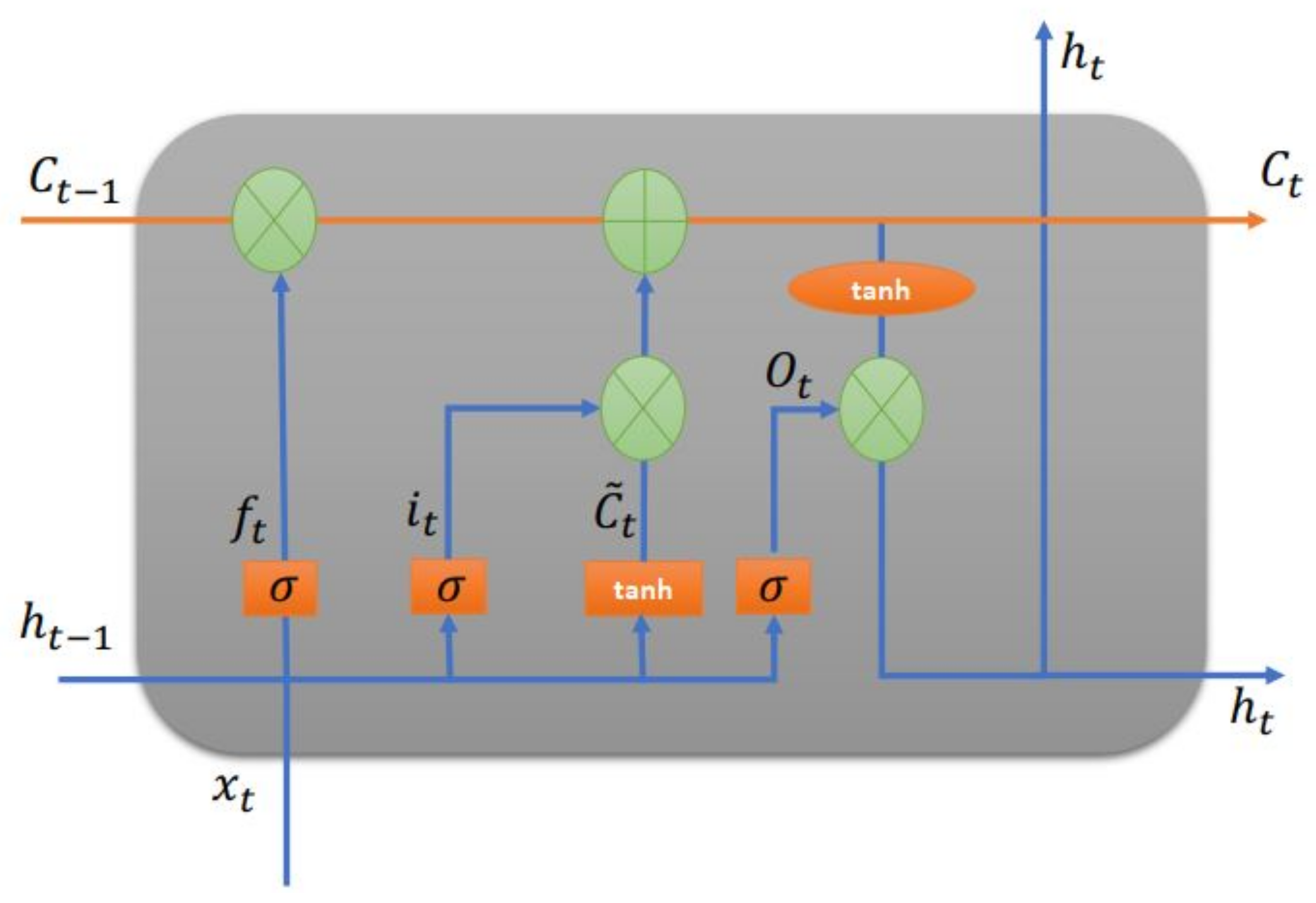
Figure 1 shows the inner design of an LSTM unit cell, according to Li and Lu [60]. Formally, the LSTM cell model is characterized as follows:

$$f_t=\sigma (x_t{W}_f+h_{t-1}{U}_f+b_f)$$

(1)

$$i_t=\sigma (x_t{W}_i+h_{t-1}{U}_i+b_i)$$

(2)

$$o_t=\sigma (x_t{W}_o+h_{t-1}{U}_o+b_o)$$

(3)

$${\tilde{C}}_t=tan[x_t{W}_C+h_{t-1}{U}_c+b_c]$$

(4)

$$C_t=\sigma (f_t\times C_{t-1}+i_t\times {\tilde{C}}_t)$$

(5)

$$h_t=tanh\left(C_t\right)\times o_t$$

(6)

Matrices $W_q$ and $U_q$ contain the weights of the input and recurrent connections, where the index can be the input gate i, output gate o, the forgetting gate f or the memory cell c, depending on the activation being calculated. $c_t\in$ ${\mathbb{R}}^h$ is not just a cell of an LSTM unit, but contains h cells of the LSTM units, while $i_t$, $o_t$ and $f_t$ represent the activations of, respectively, the input, output and forget gates, at time step t, where:

• $x_t$ ∈ ${\mathbb{R}}^d$: input vector to the LSTM unit;
• $f_t$ ∈ ${(0,1)}^h$ forget gate’s activation vector;
• $i_t$ ∈ ${(0,1)}^h$ input/update gate’s activation vector;
• $o_t$ ∈ ${(0,1)}^h$ output gate’s activation vector;
• $h_t$ ∈ ${(-1,1)}^h$ hidden state vector, also known as the output vector of the LSTM unit;
• $\widetilde{c_t}$ ∈ ${(-1,1)}^h$ cell input activation vector;
• $c_t$ ∈ ${\mathbb{R}}^d$: cell state vector.

W ∈ ${\mathbb{R}}^{h\times d}$, U ∈ ${\mathbb{R}}^{h\times h}$ and b ∈ ${\mathbb{R}}^h$ are weight matrices and bias vector parameters, which need to be learned during training. The indices d and h refer to the number of input features and number of hidden units.

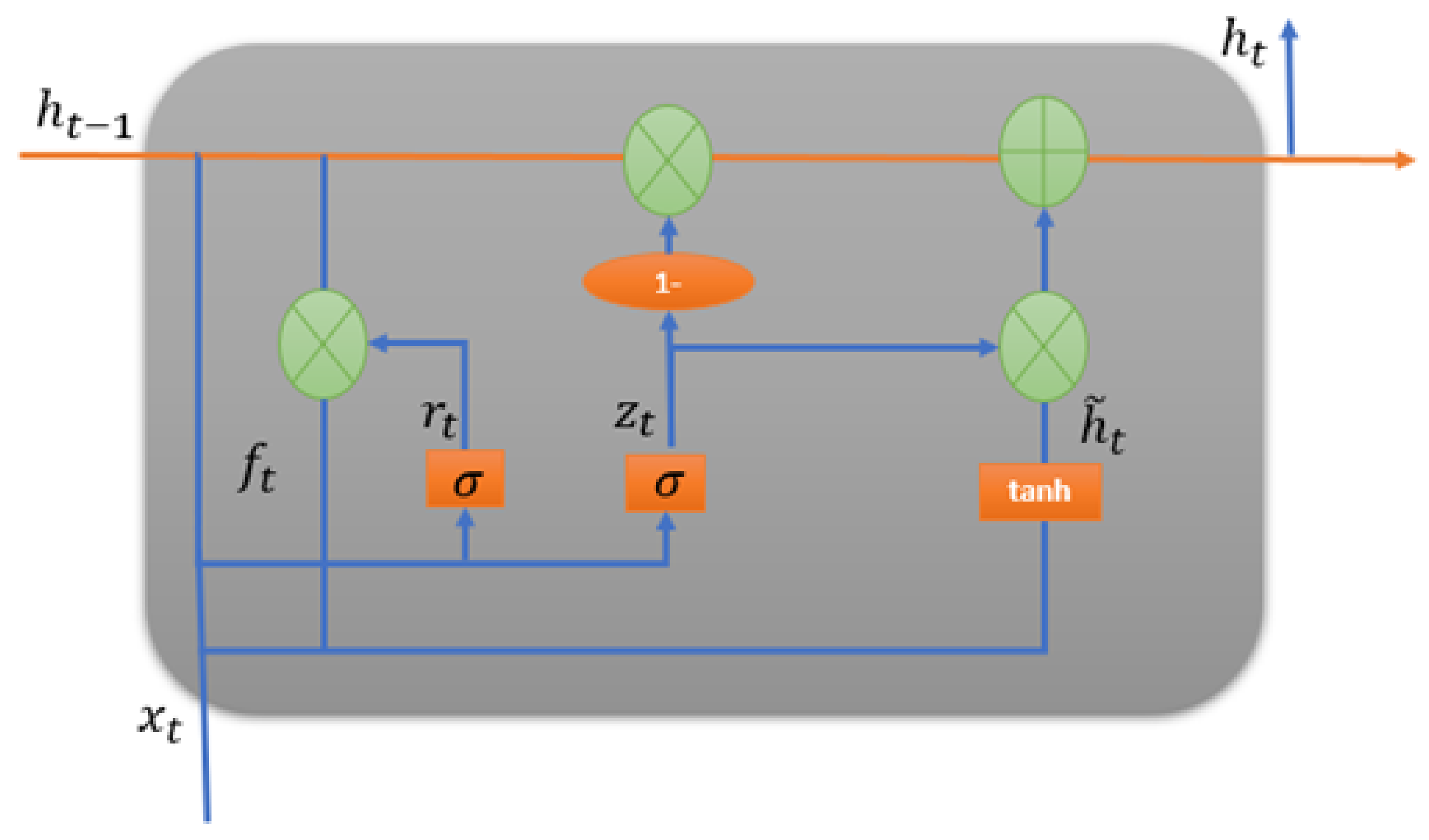
3.2. Gated Recurrent Unit

The gated recurrent unit is a special type of optimized LSTM-based recurrent neural network [61]. The GRU internal unit is similar to the LSTM internal unit [62], except that the GRU combines the incoming port and the forgetting port in LSTM into a single update port. In [63], a new system called the multi-GRU prediction system was developed based on GRU models for the planning and operation of electricity generation.

The GRU was introduced by Cho et al. [64]. Although it was inspired by the LSTM unit, it is considered simpler to calculate and implement. It retains the LSTM immunity to the vanishing gradient problem. Its internal structure is simpler and, therefore, it is also easier to train, as less calculation is required to upgrade the internal states. The update port controls the extent to which the state information from the previous moment is retained in the current state, while the reset port determines whether the current state should be combined with the previous information [64].

Figure 2 shows the internal architecture of a GRU unit cell. These are the mathematical functions used to control the locking mechanism in the GRU cell:

$$z_t=\sigma (x_t{W}^z+h_{t-1}{U}^z+b_z)$$

(7)

$$r_t=\sigma (x_t{W}^r+h_{t-1}{U}^r+b_r)$$

(8)

$${\tilde{h}}_t=tan(r_t\times h_{t-1}U+x_{t}W+b)$$

(9)

$$h_t=(1-z_t)\times {\tilde{h}}_t+z_t\times h_{t-1}$$

(10)

where $W^z,W^r,W$ denote the weight matrices for the corresponding connected input vector. $U^z,U^r,U$ represent the weight matrices of the previous time step, and $b_r,b_z$ and b are bias. The $\sigma$ denotes the logistic sigmoid function, $r_t$ denotes the reset gate, $z_t$ denotes the update gate, and $\widetilde{h_t}$ denotes the candidate hidden layer [65].

It shows that the GRU has an updated port and a reset port similar to forget and input ports on the LSTM unit. The refresh port defines how much old memory to keep, and the reset port defines how to combine the new entry with the old memory. The main difference is that the GRU fully exposes its memory content using just integration (but with an adaptive time constant controlled by the update port).

Deep learning networks are very sensitive to hyperparameters. When the hyperparameters are incorrectly set, the predicted output will produce high-frequency oscillation [66]. Important hyperparameters for GRU network models are the number of hidden units in the recurrent layers, the dropout value, and the learning rate value.

Individually, these hyperparameters can significantly influence the performance of the LSTM or GRU neural models. Studies, such as [67,68], demonstrate how important the adjustment of hyperparameters is, as it optimizes the learning process and can present good results against more complex neural network structures.

3.3. Model Evaluation

In the present experiments, LSTM and GRU neural network models are compared. To evaluate the model prediction performance, the models used were root mean square error (RMSE), mean absolute percentage error (MAPE), and mean absolute error (MAE). They are defined as follows:

$$RMSE=\sqrt{\frac{1}{n}\sum _{\begin{array}{c}t=1\end{array}}^n{(Y_t-\widehat{Y})}^2}$$

(11)

where $Y_t$ is the actual data value and $\widehat{Y}$ is the forecast obtained from the model value. The prediction error is calculated as the difference between Y and $\widehat{Y}$, i.e., the difference between the output desired and the output obtained. n is the number of samples used in the test set.

$$MAE=\frac{1}{n}\sum _{\begin{array}{c}t=1\end{array}}^n|Y_t-{\widehat{Y}}_t|$$

(12)

$$MAPE=\frac{1}{n}\sum _{\begin{array}{c}t=1\end{array}}^n\frac{|Y_t-{\widehat{Y}}_t|}{|Y_t|}$$

(13)

4. Data Preparation

The present work is a continuation of previous work, where the data from the industrial press were already studied and analyzed using LSTM models [59]. The industrial presses are monitored by six sensors, with a sampling period of 1 min. The dataset contains data samples from 1 February, 2018 to December, 2020, for a total of 1004 days. The variables monitored are (1) electric current intensity (C. intensity); (2) hydraulic unit oil level (hydraulic unit level); (3) VAT pressure; (4) motor velocity (velocity); (5) temperature at the unit hydraulic (temperature at U.H.); and (6) torque.

Figure 3 shows the plot of the raw data. As the graph shows, there are zones of typical operation and spikes of discrepant data. Figure 4 is a Q–Q plot, showing the normality of the data. As the figure shows, the data are not homogeneous. There are many discrepant samples in the extreme quantiles and the distribution of data is not linear.

Data quality is essential for developing effective modeling and planning. Data with discrepant values, as those shown in the charts, can pose difficulties to machine learning models. Therefore, data need to be processed and structured prior to analysis.

There are several treatment methods designed for this purpose, but a careful selection is needed so that information is not impaired. In the present work, the approach followed was the quantile method [59]. The quantile method removes extreme values, which are often due to sensor reading errors, stops, or other abnormal situations. After those samples are removed, it is possible to see more normal data distributions, such as those shown in Figure 5 and Figure 6.

Since the present study relies on information that exists in the samples, this gives rise to the idea of presenting the correlation that exists between the variables. That information was condensed in the correlation matrix shown in Figure 7. As the figure shows, some of the correlations are interesting, such as those observed among the current, torque, and pressure. Other correlations are very low, such as those between oil level and temperature.

5. Methods

The present study aims to compare the performance of the LSTM model and the GRU model to predict future sensor values with 30 days advance, based on a window of past values. Experiments were performed using a computer with a third generation i5 processor, with 8 GB RAM. Previous work [59] shows that LSTM can make predictions with MAPE errors down to 2.17% for current intensity, 2.71% for hydraulic unit oil level, 2.50% for torque, 7.65% for VAT pressure, 16.88% for velocity, and 3.06% for temperature, using a window of 10 days and a sampling rate of two samples per day per sensor.

In the present work, different network architectures and hyperparameters were tested, for LSTM and GRU. In both cases, the networks rely on an encoding layer, a hidden layer of variable lengths, and an output layer. The internal architecture of the LSTM and GRU units are as shown in Figure 8 and Figure 9.

The models were programmed in python, using the frameworks TensorFlow and Keras. For training, a batch size of 16 was used. Other hyperparameters, such as the activation function, when not indicated otherwise, are the TensorFlow and Keras default values.

For the experiments, the dataset was divided into train and test subsets. The test set was used for validation during the training process and for final evaluation. The samples were not included in the training set. The training set consisted of 70% of the samples and the test set contained the remaining 30% of the samples.

Experiments were performed with different resampling rates. Using aggressive resampling, the size of the dataset is greatly reduced, which increases speed and decreases the influence of outliers in the data. However, for more precision, lower resampling rates must be used.

To determine the best size for the sliding window, experiments were performed, resampling to just one sample per day, which gave a total of 1004 samples, 70% of which were used for train and 30% for test. Experiments were also performed to determine the best resample rate, showing that using one sample per hour was a good compromise between the computation required and the performance of the model, as explained in Section 6.

Different experiments were performed to compare the performance of the LSTM and the GRU, with different sets of hyperparameters. The parameters were varied and tested one-by-one. Dense search methods, such as grid-search, were not used because of the processing time required.

6. Experiments and Results

Experimental work was performed to confirm the ability of the models to learn, and then to determine the optimal hyperparameters of the LSTM and GRU.

6.1. Testing the Convergence of the Learning Process

Figure 10 shows the learning curve of a GRU model, with 40 units in the hidden layer and window of 12 samples. The graph shows the loss measured in the train and in the test set. The learning process converges and takes less than 10 epochs to reach a small loss. This is similar to previous results obtained for the LSTM [59].

Although the learning curve shows that the model learns very quickly, in less than 10 epochs, in the following experiments, the number of epochs was limited to 15.

6.2. Experiments to Determine Model Performance with Different Window Sizes

The first experiment carried out, aimed to find the optimal window for the LSTM model and for the GRU model. The experiments were performed using one sample per day. Thus, the dataset had a total of 1004 samples. The models used had 40 units in the hidden layer.

Figure 11 shows the results of the two models, using different window sizes and two different activation functions in the output layer. The RMSE is the average of all the variables. As the charts show, the GRU is always better than the LSTM, regardless of the window size or activation function used. The window size only has a small impact on the performance of the model, being the differences minimal from two to 12 days. On the other hand, the results are better when the ReLU is used at the output layer. When the sigmoid function is used, the difference in performance between the GRU and the LSTM is larger than when the ReLU function is used.

Figure 12 shows the MAPE and MAE associated with the 30 day forecast, for past windows of 2 to 12 days. The charts demonstrate that the LSTM architecture that uses a ReLU activation function in the output layer has lower errors. Using the sigmoid function, the LSTM errors are much larger. The GRU, however, in general performs better than the LSTM for all variables and activation functions. The prediction error results are much more stable for the GRU than they are for the LSTM.

Table 1. Summary of the best prediction errors obtained with the LSTM models. Window is the historical window size in days. AF is the output activation function.

			MAPE
Window-AF	C. Intensity	Hydraulic	Torque	Pressure	Velocity	Temperature
4-ReLU	2.95	2.32	3.68	8.28	14.06	2.38
6-Sigmoid	16.48	65.98	4.24	12.09	19.70	34.00
			MAE
Window-AF	C. Intensity	Hydraulic	Torque	Pressure	Velocity	Temperature
4-ReLU	0.86	1.74	0.54	1.29	0.50	0.91
6-Sigmoid	4.91	50.34	0.61	1.83	0.72	13.02

shows exact error values for the best window sizes for the LSTM model.

Table 2. Summary of the best prediction errors obtained with the GRU models. Window is the historical window size in days. AF is the output activation function.

			MAPE
Window-AF	C. Intensity	Hydraulic	Torque	Pressure	Velocity	Temperature
12-ReLU	3.63	1.95	3.53	7.74	15.99	1.92
10-Sigmoid	2.57	2.21	3.74	9.53	15.41	2.82
			MAE
Window-AF	C. Intensity	Hydraulic	Torque	Pressure	Velocity	Temperature
12-ReLU	0.77	2.20	0.44	1.49	0.55	0.86
10-Sigmoid	0.93	1.32	0.61	1.42	0.64	0.91

shows the best window sizes for the GRU model.

6.3. Experiments to Determine Model Performance with Different Resample Rates

In a second experiment, the models were tested with different resampling rates. Resampling is often used as a preprocessing method. Different techniques are used. Some of them are undersampling, in which the dataset size is reduced. This speeds up the data processing. In other cases, oversampling methods (such as data augmentation) are used in order to increase the number of samples.

In the present experiments, the dataset contains a large number of samples, so only undersampling techniques are necessary in order to reduce the number of data points. The method used was to average a number of samples, depending on the size of the dataset desired. Experiments were performed undersampling to obtain one sample per 12 h (two per day), one per six hours (four samples per day), one per each three hours, and finally one sample per hour. So the dataset size was greatly reduced.

The window sizes were the best of the previous experiments: a window size of 4 days for the LSTM and 12 days for the GRU, with the ReLU. A window size of 6 days for the LSTM and 10 days for the GRU, with the sigmoid.

Figure 13 shows the average RMSE errors for both models. As the results show, sometimes the LSTM overperformed the GRU, namely when using the sigmoid function with periods of six and three hours. However, the difference was not statistically significant. On the other hand, the GRU was able to learn in all the situations and the RMSE error was always approximately 1. So, the GRU is robust and accepts larger periods with minimal impact on the performance, while the LSTM model is much more unstable.

Figure 14 shows the MAE and MAPE errors calculated for each variable. It is possible to verify that, in general, the errors are much smaller with the sigmoid function. The LSTM model with the ReLU function is able to learn when a period of 12 h is used. When the sampling period is six hours, it seems the error gradient explodes for all variables and the errors become extremely large. For lower sampling periods, the LSTM does not learn. The GRU model continues to learn with acceptable errors.

Table 3. Summary of the best prediction errors obtained with the LSTM models, using different resampling rates.

			MAPE
Resampling-AF	C. Intensity	Hydraulic	Torque	Pressure	Velocity	Temperature
12-ReLU	2.42	2.92	3.72	10.36	17.19	2.30
			MAE
Resampling-AF	C. Intensity	Hydraulic	Torque	Pressure	Velocity	Temperature
12-ReLU	0.71	2.22	0.55	1.57	0.64	0.88

shows the best results for the LSTM model with different resampling rates.

Table 4. Summary of the best prediction errors obtained with the GRU models, using different resampling rates.

			MAPE
Resampling-AF	C. Intensity	Hydraulic	Torque	Pressure	Velocity	Temperature
1-ReLU	2.52	2.94	3.03	9.91	15.05	2.84
1-Sigmoid	2.22	2.72	2.88	9.29	12.42	2.74
			MAE
Resampling-AF	C. Intensity	Hydraulic	Torque	Pressure	Velocity	Temperature
1-ReLU	0.70	2.62	0.43	1.58	0.50	1.21
1-Sigmoid	0.65	1.99	0.43	1.41	0.48	1.03

shows the best results for the GRU model with different resampling rates.

6.4. Experiments with Different Layer Sizes

An additional experiment was performed, to compare the performance of the models with different numbers of units in the hidden layer.

Using the GRU model, it is possible to learn with a larger number of samples, and with different variations of the model units, as shown in Figure 15 and Figure 16. The LSTM was unable to learn with the resampling rate period of 1 h; therefore, results are missing. The window used in the experiments was 10 days for the sigmoid and 12 days for the ReLU, which were the optimal windows for the GRU using the ReLU and sigmoid functions, respectively.

As the charts show, the GRU, using the sigmoid activation function, achieves the lowest RMSE error with 50 units in the hidden layer. Experiments described in Section 6.3 showed that the GRU with the same parameters, with 40 units in the hidden layer, had an RMSE error of 1.06.

Table 5. Summary of the best results obtained with different numbers of units in the hidden layer.

			MAPE
Unit	C. Intensity	Hydraulic	Torque	Pressure	Velocity	Temperature
80-ReLU	2.66	4.09	3.19	10.31	13.83	3.29
50-Sigmoid	2.30	2.80	2.85	9.87	11.80	2.66
			MAE
Unit	C. Intensity	Hydraulic	Torque	Pressure	Velocity	Temperature
80-ReLU	0.78	3.02	0.47	1.58	0.55	1.25
50-Sigmoid	0.68	2.05	0.42	1.48	0.46	1.01

shows the best results for the GRU model, after the tests with different numbers of cells in the hidden layer.

6.5. Comparing Many-to-Many and One-to-Many Architectures

An additional experiment was performed, in order to determine if the models are better trained to predict all the variables at the same time (one model, six outputs—many-to-many variables) or trained to predict just one variable (six models, one output each—many-to-one variable).

This experiment was just performed for the GRU, which presented the best results in the previous experiments.

According to the graphs presented in Figure 17, it is clear that architecture ’many-to-many’ presents slightly better results. Therefore, there is no advantage in training one model to predict each variable.

6.6. Tests with Different Activation Functions in the Hidden Layer

An additional step was to test combinations of different activation functions, for the hidden and output layers of the GRU. The activation functions tested were sigmoid, hyperbolic tangent (tanh), and ReLU. Figure 18 shows a chart with the average RMSE of the models. Globally, ReLU in the hidden layer and tanh for the output are the best models, even though ReLU–sigmoid and ReLU–ReLU are closely behind.

Table 6. Average RMSE obtained for the six variables, with different activation functions, calculated after the values were smoothed with a median filter.

			RMSE
Function	C. Intensity	Hydraulic	Torque	Pressure	Velocity	Temperature
ReLU–ReLU	0.96	3.48	0.42	1.90	0.84	1.90
ReLU–Sigmoid	0.93	1.72	0.53	1.60	0.79	1.19
ReLU–Tanh	0.83	2.47	0.48	1.70	0.76	1.25
Sigmoid–Sigmoid	0.98	6.40	0.45	2.14	0.89	1.35
Sigmoid–ReLU	1.22	4.87	0.43	1.86	0.74	1.31
Sigmoid–Tanh	1.19	7.38	0.45	2.03	0.78	1.35
Tanh–Tanh	1.36	7.84	0.44	2.24	0.91	1.35
Tanh–ReLU	0.86	7.3	0.42	1.91	0.76	1.41

shows the RMSE error for the different combinations of activation functions, for each variable. As the table shows, different variables may benefit from different functions, although, in general, a first layer of ReLU and a second layer of ReLU, sigmoid, or tanh are good choices.

The values shown in Table 6 are calculated for the raw output predicted. However, the raw output values have some sharp variations, which are undesirable for a predictive system. Therefore, the values were filtered and smoothed using a median filter. Figure 19 shows plots of selected results, where the signals and predictions were filtered with a rolling median filter, with a rolling window of 48 h.

Table 7. Average RMSE obtained for the six variables after the average clean method, with different activation functions using the GRU model.

			RMSE
Function	C. Intensity	Hydraulic	Torque	Pressure	Velocity	Temperature
ReLU–ReLU	0.71	3.33	0.28	1.36	0.66	0.80
ReLU–Sigmoid	0.61	1.58	0.39	1.08	0.61	0.78
ReLU–Tanh	0.54	2.33	0.35	1.13	0.54	0.82
Sigmoid–Sigmoid	0.73	6.36	0.30	1.70	0.68	0.94
Sigmoid–ReLU	1.03	4.80	0.28	1.32	0.50	0.89
Sigmoid–Tanh	0.98	7.35	0.29	1.53	0.54	0.94
Tanh–Tanh	1.18	7.81	0.29	1.80	0.70	0.96

shows the MSE errors calculated after smoothing. As the table shows, after smoothing, the prediction errors decrease.

Figure 19 shows examples of plots of different prediction lines in part of the test set. As the results show, in some cases the ReLU–tanh combination is the best, while in other cases, the ReLU–sigmoid offers better performance. The ReLU–tanh combination is better, in general, but in the case of temperature, the sigmoid output shows the best performance.

7. Discussion

Based on studies presented in the state of the art, it is possible to verify the usefulness of deep networks for prediction in time series variables. The area of prediction using deep neural networks has grown fast, due to the development of new models and the evolution of calculation power. LSTM and GRU models are two of the best forecast models. They have gained popularity recently, even though most of the state-of-the-art models are more traditional architectures.

The GRU network is simpler than the LSTM, supports higher resampling rates, and it can work on smaller and larger datasets. The experiments performed showed that the best results are based on the GRU neural network: it is easier and faster to train and achieve good results. A GRU network, with encoding and decoding layers, is able to forecast future behavior of an industrial paper press, 30 days in advance, with MAPE in general less than 10%.

An optimized GRU model offers better results with a 12-day sampling sliding window, with a sampling period of 1 h, and 50 units in the hidden layer. The best activation functions depend on the model. However, the ReLU–tanh is perhaps one of the best models, on average.

The results also demonstrate that training the models using just one output variable, thus optimizing a model for each variable separately, is not advantageous when compared to training one model to predict all six variables at the same time.

The present work shows that a GRU network, with encoding and decoding layers, can be used to anticipate future behavior of an industrial paper press. It shows better overall performance, with less processing requirements, when compared to an equivalent LSTM model. To the best of the authors’ knowledge, this is the first time such a study has been made. The prediction errors are smaller than those presented by the LSTM neural network and the GRU is more immune to exploding or vanishing gradient problems, so it learns in a wider range of configurations.

Compared to the literature, previous research has shown that the GRU is often the best predictor [69,70,71]. However, those studies were performed for univariate data only. The present work uses six variables in a time series and compares the multivariate and the univariate models. In [72], the model that presents the lowest RMSE is the ARIMA. However, that is just for a small dataset and forecast with 6 samples advance. In [44,73], forecasting models with LSTM, including encoding and decoding, are proposed, although not compared to GRU.

8. Conclusions

In the industrial world, it is important to minimize downtime. Equipment downtime, due to failure or curative maintenance, represents hours of production lost. To solve this problem, predictive maintenance is, nowadays, the best solution. Artificial intelligence models have been employed, aimed at anticipating the future behavior of machines and, therefore, avoiding potential failures.

The study presented in this paper compares the performance of LSTM and GRU models, predicting future values of six sensors, installed at an industrial paper press 30 days in advance.

The GRU models, in general, operate with less data and offer better results, with a wider range of parameters, as demonstrated in the case study based on pulp presses.

Future work will include testing the performance of the GRU with different time gaps, in order to determine the best performance for different time gaps.

References

- Bousdekis, A.; Lepenioti, K.; Apostolou, D.; Mentzas, G. A review of data-driven decision-making methods for industry 4.0 maintenance applications. Electronics 2021, 10, 828. [Google Scholar] [CrossRef]
- Pech, M.; Vrchota, J.; Bednář, J. Predictive maintenance and intelligent sensors in smart factory: Review. Sensors 2021, 21, 1470. [Google Scholar] [CrossRef]
- Martins, A.; Fonseca, I.; Farinha, J.T.; Reis, J.; Cardoso, A.J.M. Maintenance Prediction through Sensing Using Hidden Markov Models—A Case Study. Appl. Sci. 2021, 11, 7685. [Google Scholar] [CrossRef]
- Hao, Q.; Xue, Y.; Shen, W.; Jones, B.; Zhu, J. A Decision Support System for Integrating Corrective Maintenance, Preventive Maintenance, and Condition-Based Maintenance; Construction Research Congress: Banff, AB, Canada, 2012; pp. 470–479. [Google Scholar] [CrossRef] [Green Version]
- Chen, C.; Liu, Y.; Wang, S.; Sun, X.; Di Cairano-Gilfedder, C.; Titmus, S.; Syntetos, A.A. Predictive maintenance using cox proportional hazard deep learning. Adv. Eng. Inform. 2020, 44, 101054. [Google Scholar] [CrossRef]
- Sherwin, D.J. Age-based opportunity maintenance. J. Qual. Maint. Eng. 1999, 5, 221–235. [Google Scholar] [CrossRef]
- Bianchi, F.M.; De Santis, E.; Rizzi, A.; Sadeghian, A. Short-Term Electric Load Forecasting Using Echo State Networks and PCA Decomposition. IEEE Access 2015, 3, 1931–1943. [Google Scholar] [CrossRef]
- Pati, J.; Kumar, B.; Manjhi, D.; Shukla, K.K. A Comparison Among ARIMA, BP-NN, and MOGA-NN for Software Clone Evolution Prediction. IEEE Access 2017, 5, 11841–11851. [Google Scholar] [CrossRef]
- Akaike, H. Autoregressive Model Fitting for Control. In Selected Papers of Hirotugu Akaike; Parzen, E., Tanabe, K., Kitagawa, G., Eds.; Springer Series in Statistics; Springer: Berlin/Heidelberg, Germany, 1998; pp. 153–170. [Google Scholar] [CrossRef]
- Ray, S.; Das, S.S.; Mishra, P.; Al Khatib, A.M.G. Time Series SARIMA Modelling and Forecasting of Monthly Rainfall and Temperature in the South Asian Countries. Earth Syst. Environ. 2021, 5, 531–546. [Google Scholar] [CrossRef]
- Wang, K.; Wang, Y. How AI Affects the Future Predictive Maintenance: A Primer of Deep Learning. In Advanced Manufacturing and Automation VII; Wang, K., Wang, Y., Strandhagen, J.O., Yu, T., Eds.; Notas de aula sobre engenharia elétrica; Springer: Berlin/Heidelberg, Germany, 2018; pp. 1–9. [Google Scholar] [CrossRef]
- Carvalho, T.P.; Soares, F.A.A.M.N.; Vita, R.; da Francisco, P.R.; Basto, J.P.; Alcalá, S.G.S. A systematic literature review of machine learning methods applied to predictive maintenance. Comput. Ind. Eng. 2019, 137, 106024. [Google Scholar] [CrossRef]
- Wuest, T.; Weimer, D.; Irgens, C.; Thoben, K.D. Machine learning in manufacturing: Advantages, challenges, and applications. Prod. Manuf. Res. 2016, 4, 23–45. [Google Scholar] [CrossRef] [Green Version]
- Soares, S.G. Ensemble Learning Methodologies for Soft Sensor Development in Industrial Processes. Ph.D. Thesis, Faculty of Science and Technology of the University of Coimbra, Coimbra, Portugal, 2015. [Google Scholar]
- Shin, J.H.; Jun, H.B.; Kim, J.G. Dynamic control of intelligent parking guidance using neural network predictive control. Comput. Ind. Eng. 2018, 120, 15–30. [Google Scholar] [CrossRef]
- Paolanti, M.; Romeo, L.; Felicetti, A.; Mancini, A.; Frontoni, E.; Loncarski, J. Machine Learning approach for Predictive Maintenance in Industry 4.0. In Proceedings of the 2018 14th IEEE/ASME International Conference on Mechatronic and Embedded Systems and Applications (MESA), Oulu, Finland, 2–4 July 2018; pp. 1–6. [Google Scholar] [CrossRef]
- Bangalore, P.; Tjernberg, L.B. An Artificial Neural Network Approach for Early Fault Detection of Gearbox Bearings. IEEE Trans. Smart Grid 2015, 6, 980–987. [Google Scholar] [CrossRef]
- Sugiyarto, A.W.; Abadi, A.M. Prediction of Indonesian Palm Oil Production Using Long Short-Term Memory Recurrent Neural Network (LSTM-RNN). In Proceedings of the 2019 1st International Conference on Artificial Intelligence and Data Sciences (AiDAS), Ipoh, Malaysia, 19 September 2019; pp. 53–57. [Google Scholar] [CrossRef]
- Lara-Benítez, P.; Carranza-García, M.; Luna-Romera, J.M.; Riquelme, J.C. Temporal convolutional networks applied to energy-related time series forecasting. Appl. Sci. 2020, 10, 2322. [Google Scholar] [CrossRef] [Green Version]
- Yeomans, J.; Thwaites, S.; Robertson, W.S.; Booth, D.; Ng, B.; Thewlis, D. Simulating Time-Series Data for Improved Deep Neural Network Performance. IEEE Access 2019, 7, 131248–131255. [Google Scholar] [CrossRef]
- Yu, Z.; Moirangthem, D.S.; Lee, M. Continuous Timescale Long-Short Term Memory Neural Network for Human Intent Understanding. Front. Neurorobot. 2017, 11, 42. [Google Scholar] [CrossRef]
- Aydin, O.; Guldamlasioglu, S. Using LSTM Networks to Predict Engine Condition on Large Scale Data Processing Framework. In Proceedings of the 4th International Conference on Electrical and Electronic Engineering (ICEEE), Ankara, Turkey, 8–10 April 2017; pp. 281–285. [Google Scholar] [CrossRef]
- Dong, D.; Li, X.Y.; Sun, F.Q. Life prediction of jet engines based on LSTM-recurrent neural networks. In Proceedings of the 2017 Prognostics and System Health Management Conference (PHM-Harbin), Harbin, China, 9–12 July 2017; pp. 1–6. [Google Scholar] [CrossRef]
- Baptista, M.; Sankararaman, S.; de Medeiros, I.P.; Nascimento, C.; Prendinger, H.; Henriques, E.M.P. Forecasting fault events for predictive maintenance using data-driven techniques and ARIMA modeling. Comput. Ind. Eng. 2018, 115, 41–53. [Google Scholar] [CrossRef]
- Wang, J.; Zhang, T. Degradation prediction method by use of autoregressive algorithm. In Proceedings of the 2008 IEEE International Conference on Industrial Technology, Chengdu, China, 21–24 April 2008; pp. 1–6. [Google Scholar] [CrossRef]
- Cruz, S.; Paulino, A.; Duraes, J.; Mendes, M. Real-Time Quality Control of Heat Sealed Bottles Using Thermal Images and Artificial Neural Network. J. Imaging 2021, 7, 24. [Google Scholar] [CrossRef]
- Su, C.T.; Yang, T.; Ke, C.M. A neural-network approach for semiconductor wafer post-sawing inspection. IEEE Trans. Semicond. Manuf. 2002, 15, 260–266. [Google Scholar] [CrossRef]
- Zhang, J.T.; Xiao, S. A note on the modified two-way MANOVA tests. Stat. Probab. Lett. 2012, 82, 519–527. [Google Scholar] [CrossRef]
- Carnero, M. An evaluation system of the setting up of predictive maintenance programmes. Reliab. Eng. Syst. Saf. 2006, 91, 945–963. [Google Scholar] [CrossRef]
- Bansal, D.; Evans, D.J.; Jones, B. A real-time predictive maintenance system for machine systems. Int. J. Mach. Tools Manuf. 2004, 44, 759–766. [Google Scholar] [CrossRef]
- Ghaboussi, J.; Joghataie, A. Active Control of Structures Using Neural Networks. J. Eng. Mech. 1995, 121, 555–567. [Google Scholar] [CrossRef]
- Bruneo, D.; De Vita, F. On the Use of LSTM Networks for Predictive Maintenance in Smart Industries. In Proceedings of the 2019 IEEE International Conference on Smart Computing (SMARTCOMP), Washington, DC, USA, 12–15 June 2019; pp. 241–248. [Google Scholar] [CrossRef]
- Wang, L.; Hope, A.D. Fault diagnosis: Bearing fault diagnosis using multi-layer neural networks. Insight-Non-Destr. Test. Cond. Monit. 2004, 46, 451–455. [Google Scholar] [CrossRef]
- Kittisupakorn, P.; Thitiyasook, P.; Hussain, M.; Daosud, W. Neural network based model predictive control for a steel pickling process. J. Process Control 2009, 19, 579–590. [Google Scholar] [CrossRef]
- Yasaka, K.; Akai, H.; Kunimatsu, A.; Kiryu, S.; Abe, O. Deep learning with convolutional neural network in radiology. Jpn. J. Radiol. 2018, 36, 257–272. [Google Scholar] [CrossRef] [PubMed]
- Krizhevsky, A.; Sutskever, I.; Hinton, G.E. Imagenet classification with deep convolutional neural networks. Adv. Neural Inf. Process. Syst. 2012, 25, 1097–1105. [Google Scholar] [CrossRef]
- Ni, H.G.; Wang, J.Z. Prediction of compressive strength of concrete by neural networks. Cem. Concr. Res. 2000, 30, 1245–1250. [Google Scholar] [CrossRef]
- Partovi, F.Y.; Anandarajan, M. Classifying inventory using an artificial neural network approach. Comput. Ind. Eng. 2002, 41, 389–404. [Google Scholar] [CrossRef]
- Fonseca, D.; Navaresse, D.; Moynihan, G. Simulation metamodeling through artificial neural networks. Eng. Appl. Artif. Intell. 2003, 16, 177–183. [Google Scholar] [CrossRef]
- Guo, Y.; Wu, Z.; Ji, Y. A Hybrid Deep Representation Learning Model for Time Series Classification and Prediction. In Proceedings of the 2017 3rd International Conference on Big Data Computing and Communications (BIGCOM), Chengdu, China, 10–11 August 2017; pp. 226–231. [Google Scholar] [CrossRef]
- Liu, Y.; Duan, W.; Huang, L.; Duan, S.; Ma, X. The input vector space optimization for LSTM deep learning model in real-time prediction of ship motions. Ocean Eng. 2020, 213, 107681. [Google Scholar] [CrossRef]
- Sakalle, A.; Tomar, P.; Bhardwaj, H.; Acharya, D.; Bhardwaj, A. A LSTM based deep learning network for recognizing emotions using wireless brainwave driven system. Expert Syst. Appl. 2021, 173, 114516. [Google Scholar] [CrossRef]
- Wang, Q.; Bu, S.; He, Z. Achieving Predictive and Proactive Maintenance for High-Speed Railway Power Equipment with LSTM-RNN. IEEE Trans. Ind. Inform. 2020, 16, 6509–6517. [Google Scholar] [CrossRef]
- Park, S.H.; Kim, B.; Kang, C.M.; Chung, C.C.; Choi, J.W. Sequence-to-Sequence Prediction of Vehicle Trajectory via LSTM Encoder-Decoder Architecture. In Proceedings of the 2018 IEEE Intelligent Vehicles Symposium (IV), Changshu, China, 26–30 June 2018; pp. 1672–1678. [Google Scholar] [CrossRef] [Green Version]
- Essien, A.; Giannetti, C. A Deep Learning Model for Smart Manufacturing Using Convolutional LSTM Neural Network Autoencoders. IEEE Trans. Ind. Inform. 2020, 16, 6069–6078. [Google Scholar] [CrossRef] [Green Version]
- Soloway, D.; Haley, P.J. Neural generalized predictive control. In Proceedings of the 1996 IEEE International Symposium on Intelligent Control, Dearborn, MI, USA, 15–18 September 1996; pp. 277–282. [Google Scholar] [CrossRef]
- Hochreiter, S.; Schmidhuber, J. Long Short-Term Memory. Neural Comput. 1997, 9, 1735–1780. [Google Scholar] [CrossRef] [PubMed]
- Sak, H.; Senior, A.W.; Beaufays, F. Long sHort-Term Memory Recurrent Neural Network Architectures for Large Scale Acoustic Modeling. 2014. Available online: https://static.googleusercontent.com/media/research.google.com/en//pubs/archive/43905.pdf (accessed on 20 September 2021).
- Dahl, G.; Yu, D.; Deng, L.; Acero, A. Context-dependent pre-trained deep neural networks for large-vocabulary speech recognition. IEEE Trans. Audio Speech Lang. Process. 2012, 20, 30–42. [Google Scholar] [CrossRef] [Green Version]
- Alharbi, R.; Magdy, W.; Darwish, K.; AbdelAli, A.; Mubarak, H. Part-of-Speech Tagging for Arabic Gulf Dialect Using Bi-LSTM. In Proceedings of the Eleventh International Conference on Language Resources and Evaluation (LREC 2018), Miyazaki, Japan, 7–12 May 2018; European Language Resources Association (ELRA): Luxembourg, 2018. [Google Scholar]
- Zaremba, W.; Sutskever, I.; Vinyals, O. Recurrent Neural Network Regularization. arXiv 2015, arXiv:1409.2329. [Google Scholar]
- Luong, M.T.; Sutskever, I.; Le, Q.V.; Vinyals, O.; Zaremba, W. Addressing the Rare Word Problem in Neural Machine Translation. arXiv 2015, arXiv:1410.8206. [Google Scholar]
- Lasko, T.A.; Denny, J.C.; Levy, M.A. Computational Phenotype Discovery Using Unsupervised Feature Learning over Noisy, Sparse, and Irregular Clinical Data. PLoS ONE 2013, 8, e66341. [Google Scholar] [CrossRef]
- Bengio, Y. Learning Deep Architectures for AI; Now Publishers Inc.: Hanover, MA, USA, 2009. [Google Scholar]
- Vincent, P.; Larochelle, H.; Bengio, Y.; Manzagol, P.A. Extracting and composing robust features with denoising autoencoders. In Proceedings of the 25th International Conference on Machine Learning, Association for Computing Machinery, Helsinki, Finland, 5–9 July 2008; pp. 1096–1103. [Google Scholar] [CrossRef] [Green Version]
- Lee, H.; Pham, P.; Largman, Y.; Ng, A. Unsupervised feature learning for audio classification using convolutional deep belief networks. Adv. Neural Inf. Process. Syst. 2009, 22, 1096–1104. [Google Scholar]
- Kriegeskorte, N.; Golan, T. Neural network models and deep learning. Curr. Biol. 2019, 29, R231–R236. [Google Scholar] [CrossRef]
- Zhang, L.; Yang, F.; Daniel Zhang, Y.; Zhu, Y.J. Road crack detection using deep convolutional neural network. In Proceedings of the 2016 IEEE International Conference on Image Processing (ICIP), Phoenix, AZ, USA, 25–28 September 2016; pp. 3708–3712, ISSN: 2381-8549. [Google Scholar] [CrossRef]
- Mateus, B.C.; Mendes, M.; Farinha, J.T.; Cardoso, A.M. Anticipating Future Behavior of an Industrial Press Using LSTM Networks. Appl. Sci. 2021, 11, 6101. [Google Scholar] [CrossRef]
- Li, Y.; Lu, Y. LSTM-BA: DDoS Detection Approach Combining LSTM and Bayes. In Proceedings of the 2019 Seventh International Conference on Advanced Cloud and Big Data (CBD), Suzhou, China, 21–22 September 2019; pp. 180–185. [Google Scholar] [CrossRef]
- Santra, A.S.; Lin, J.L. Integrating Long Short-Term Memory and Genetic Algorithm for Short-Term Load Forecasting. Energies 2019, 12, 2040. [Google Scholar] [CrossRef] [Green Version]
- Chung, J.; Gulcehre, C.; Cho, K.; Bengio, Y. Empirical Evaluation of Gated Recurrent Neural Networks on Sequence Modeling. arXiv 2014, arXiv:1412.3555. [Google Scholar]
- Li, W.; Logenthiran, T.; Woo, W.L. Multi-GRU prediction system for electricity generation’s planning and operation. IET Gener. Transm. Distrib. 2019, 13, 1630–1637. [Google Scholar] [CrossRef]
- Cho, K.; van Merrienboer, B.; Bahdanau, D.; Bengio, Y. On the Properties of Neural Machine Translation: Encoder-Decoder Approaches. arXiv 2014, arXiv:1409.1259. [Google Scholar]
- Lynn, H.M.; Pan, S.B.; Kim, P. A Deep Bidirectional GRU Network Model for Biometric Electrocardiogram Classification Based on Recurrent Neural Networks. IEEE Access 2019, 7, 145395–145405. [Google Scholar] [CrossRef]
- Chai, M.; Xia, F.; Hao, S.; Peng, D.; Cui, C.; Liu, W. PV Power Prediction Based on LSTM with Adaptive Hyperparameter Adjustment. IEEE Access 2019, 7, 115473–115486. [Google Scholar] [CrossRef]
- Reimers, N.; Gurevych, I. Optimal Hyperparameters for Deep LSTM-Networks for Sequence Labeling Tasks. arXiv 2017, arXiv:1707.06799. [Google Scholar]
- Merity, S.; Keskar, N.S.; Socher, R. An Analysis of Neural Language Modeling at Multiple Scales. arXiv 2018, arXiv:1803.08240. [Google Scholar]
- Kumar, S.; Hussain, L.; Banarjee, S.; Reza, M. Energy Load Forecasting using Deep Learning Approach-LSTM and GRU in Spark Cluster. In Proceedings of the Fifth International Conference on Emerging Applications of Information Technology (EAIT), Kolkata, India, 12–13 January 2018; pp. 1–4. [Google Scholar] [CrossRef]
- Fu, R.; Zhang, Z.; Li, L. Using LSTM and GRU neural network methods for traffic flow prediction. In Proceedings of the 2016 31st Youth Academic Annual Conference of Chinese Association of Automation (YAC), Wuhan, China, 11–13 November 2016; pp. 324–328. [Google Scholar] [CrossRef]
- Shahid, F.; Zameer, A.; Muneeb, M. Predictions for COVID-19 with deep learning models of LSTM, GRU and Bi-LSTM. Chaos Solitons Fractals 2020, 140, 110212. [Google Scholar] [CrossRef]
- Yamak, P.T.; Yujian, L.; Gadosey, P.K. A Comparison between ARIMA, LSTM, and GRU for Time Series Forecasting. In Proceedings of the 2019 2nd International Conference on Algorithms, Computing and Artificial Intelligence, Sanya, China, 20–22 December 2019; Association for Computing Machinery: New York, NY, USA, 2019; pp. 49–55. [Google Scholar] [CrossRef]
- Du, S.; Li, T.; Yang, Y.; Horng, S.J. Multivariate time series forecasting via attention-based encoder–decoder framework. Neurocomputing 2020, 388, 269–279. [Google Scholar] [CrossRef]
Figure 1.
The cell structure of a long short-term memory unit.
Figure 2.
The cell structure of a gated recurrent unit.
Figure 3.
Plot of the sensor variables before applying data cleaning treatment. Many extreme values are visible for many variables, namely the hydraulic oil level and temperature.
Figure 4.
Q–Q plots of the sensor values before data cleaning treatment being applied.
Figure 5.
Sensor variables after applying data cleaning treatment. Many extreme values were removed.
Figure 6.
Q–Q plots of the sensor values after data cleaning treatment applied.
Figure 7.
Correlation matrix, showing the correlation between all variables.
Figure 8.
Base architecture of the LSTM model used.
Figure 9.
Base architecture of the GRU model used.
Figure 10.
Learning curve of a GRU model, showing the loss measured in the train and test set during the first 14 epochs.
Figure 11.
RMSE values for LSTM and GRU models, with different window sizes and activation functions for the output layer.
Figure 12.
MAPE and MAE errors, for each variable, using ReLU and sigmoid activation functions, for window sizes of 2, 4, 6, 8, 10, and 12 days, using one sample per day. Exact values are shown in