A Novel MPPT Technique Based on Mutual Coordination between Two PV Modules/Arrays

Abstract

A novel maximum power point tracking (MPPT) technique based on mutual coordination of two photovoltaic (PV) modules/arrays has been proposed for distributed PV (DPV) systems. The proposed technique works in two stages. Under non-mismatch conditions between PV modules/arrays, superior performance stage 1 is active, which rectifies the issues inherited by the perturb and observe ($P\&O$) MPPT. In this stage, the technique revolves around the perturb and observe ($P\&O$) algorithm containing an intelligent mechanism of leader and follower between two arrays. In shading conditions, stage 2 is on, and it works like conventional $P\&O$. Graphical analysis of the proposed technique has been presented under different weather conditions. Simulations of different algorithms have been performed in Matlab/Simulink. Simulation results of the proposed technique compliment the graphical analysis and show a superior performance and a fast response as compared to others, thus increasing the efficiency of distributed PV systems.

1. Introduction

PV systems stand as one of the best renewable sources because of continuous technological advancement, reduced cost and a reliable source. For obtaining the desired power and voltage levels, PV modules are connected in series-parallel configuration. However, the PV plants also inherit drawbacks, such as: (1) non-linear current vs voltage (I-V) characteristics [1]; (2) non-optimal performance under partial shading conditions [2]. Under these conditions, to extract maximum power from the PV system, the maximum power point tracker (MPPT) mechanism is deployed along with suitable connection configurations. The MPPT method is used in all kinds of PV topology.

Recently, distributed PV (DPV) system topology, shown in Figure 1, has gained importance compared to centralized PV (CPV) system illustrated in Figure 2. DPV utilizes separate dc-dc converters for each array, thus enabling it to work better than the CPV under all weather conditions [3,4]. DPV is considered a powerful solution against the shading effects [5]. Moreover, it enables flexible plant expansion, maintenance and fault detection [6,7,8]. However, the use of DPV demands topology specific MPPT methods to harness the maximum available power as explained in [9,10]. These methods vary from basic methods such as perturb and observe ($P\&O$) [11], incremental conductance to advanced particle swarm optimization (PSO) [12,13] and neural networks and so forth. However, $P\&O$ is the most widely used technique because of its low complexity, low cost and ease of implementation [14]. Therefore, this technique has the tendency to become confused under rapid changing environmental conditions and oscillates around the maximum power point (MPP) [15,16]. Moreover, this method is prone to the noise in the voltage and current and, therefore, the designer has to be vigilant in choosing the optimum perturbation amplitude and frequency [17]. The $P\&O$ MPPT has been optimized for various aspects including: (1) the use of variable perturbation size [18]; (2) adaptive perturbation frequency [19]; (3) drift control mechanism [20]; (4) reduced steady state power oscillations [21]; (5) implementation using artificial intelligence and optimization algorithms [22]; (6) hybrid solutions with $P\&O$ and other MPPT methods [23,24,25]. However, these efforts are based on the use of single/two stage power processing system with centralized PV plant.

The literature review reveals that there is no significant example of $P\&O$ optimization with DPV architecture. This paper proposes a new MPPT technique based on DPV architecture and an attempt to remove the shortcomings inherited by the conventional $P\&O$ method. The proposed technique is tested through computer aided experiments covering many weather scenarios and superior performance is witnessed in uniform and partial shading conditions.

2. Distributed PV Systems and MPPT Techniques

A centralized PV plant can provide only single cumulative information of all the PV modules at a given instant. However, a distributed PV plant can provide much information at any instant as all PV modules are not directly connected to each other as shown in Figure 1. Therefore, the MPPT designer has the opportunity to gather separate information from two similar PV modules/arrays and then performs the decisions by cross referencing their data. The proposed technique utilizes the same scheme; however, this requires two assumptions [6].

2.1. Assumptions

For a healthy comparison between two equal sized but separate PV modules/arrays, two conditions are required: (1) I-V curve of two PV arrays should be similar [6] and (2) Two PV arrays should be under the same weather conditions, that is, the same irradiance and temperature [6]. These days, condition no 1 is not very critical thanks to technological advancements. Normally, identical PV modules are connected to form an array for better efficiency. Even in two identical PV modules, the I-V curves differ by very few percent [20,21,26]. On the other hand, global I-V curves of two large PV arrays virtually coincide [27]. Working with a single PV module or small PV arrays, condition no 2 works well, as the chances of shading and different weather are low because of less distance. With large PV arrays, condition no 2 can produce few concerns but condition no 1 is well under control.

2.2. MPPT Techniques

Few MPPT techniques [6,27,28] utilize this scheme, but they adopted an incremental conductance based approach. A major concern with these techniques is that they critically need both conditions otherwise their techniques become hampered. The proposed technique adopts the mechanism of $P\&O$ and is not very critical about the two conditions. It works optimally if the two conditions occur, but works like the conventional $P\&O$ method if the two conditions are not there.

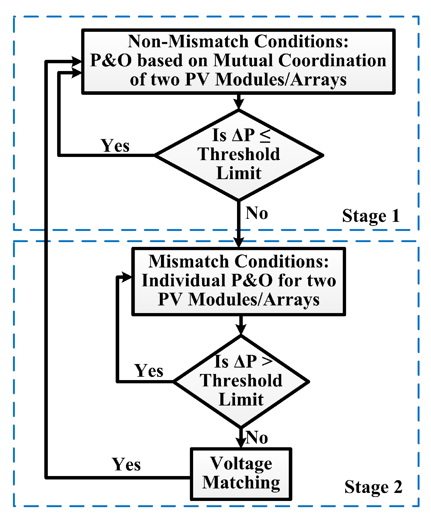
3. Basic Philosophy of Proposed Technique

The proposed MPPT technique is based on the $P\&O$ mechanism operating between two similar PV arrays. It has two stages, as shown in Figure 3. Stage 1, which is for non-mismatch conditions, calculates the power difference ($\Delta P$) between two PV modules/arrays. If $\Delta P$ becomes greater than the threshold limit, it indicates a mismatch condition; consequently it switches to stage 2. Stage 2 is designed to addresses the mismatch conditions. Here, the algorithm performs $P\&O$ for each array while monitoring the power condition during each iteration. Whenever $\Delta P$ comes within the threshold limit, then the algorithm sets an equal voltage operating point and returns back to stage 1.

Selection of Threshold Limit Values

The PV module datasheet reports the power tolerance between 0 to 5 W or +/−3% to the rated power. Researchers have calculated the power difference between two similar PV modules due to manufacturing mismatch and have concluded that such losses are negligible for large arrays [29,30]. The threshold limit (THL) is calculated either through way 1 or way 2. The only difference between way 1 and way 2 is that the PV array with the relatively greater power is the deciding factor. First, a threshold value (TH) is selected from Table II depending upon the size of PV plant. Consider that a threshold value of 0.5% is selected:

$$TH=\frac{0.5}{100}$$

(1)

Stage 1: way 1, that is, if PL is greater or equal:

$$THL=TH\times PL$$

(2)

$$\Delta P=PL-PF$$

(3)

Stage 1: way 2 i.e., if PF is greater then the expression for THL remains same but

$$\Delta P=PF-PL,$$

(4)

where THL is the threshold limit and $\Delta P$ is the power difference. Using the information given in [29,30], the threshold value for the proposed algorithm for a different array size is given in

Table 1. Threshold Value Selection.

No of Modules Per Array	Threshold Value Range
Greater than 12	0.3 to 0.7%
Greater than 1 and less than 12	0.8% to 1.3%
1	1.4% to 1.7%

.

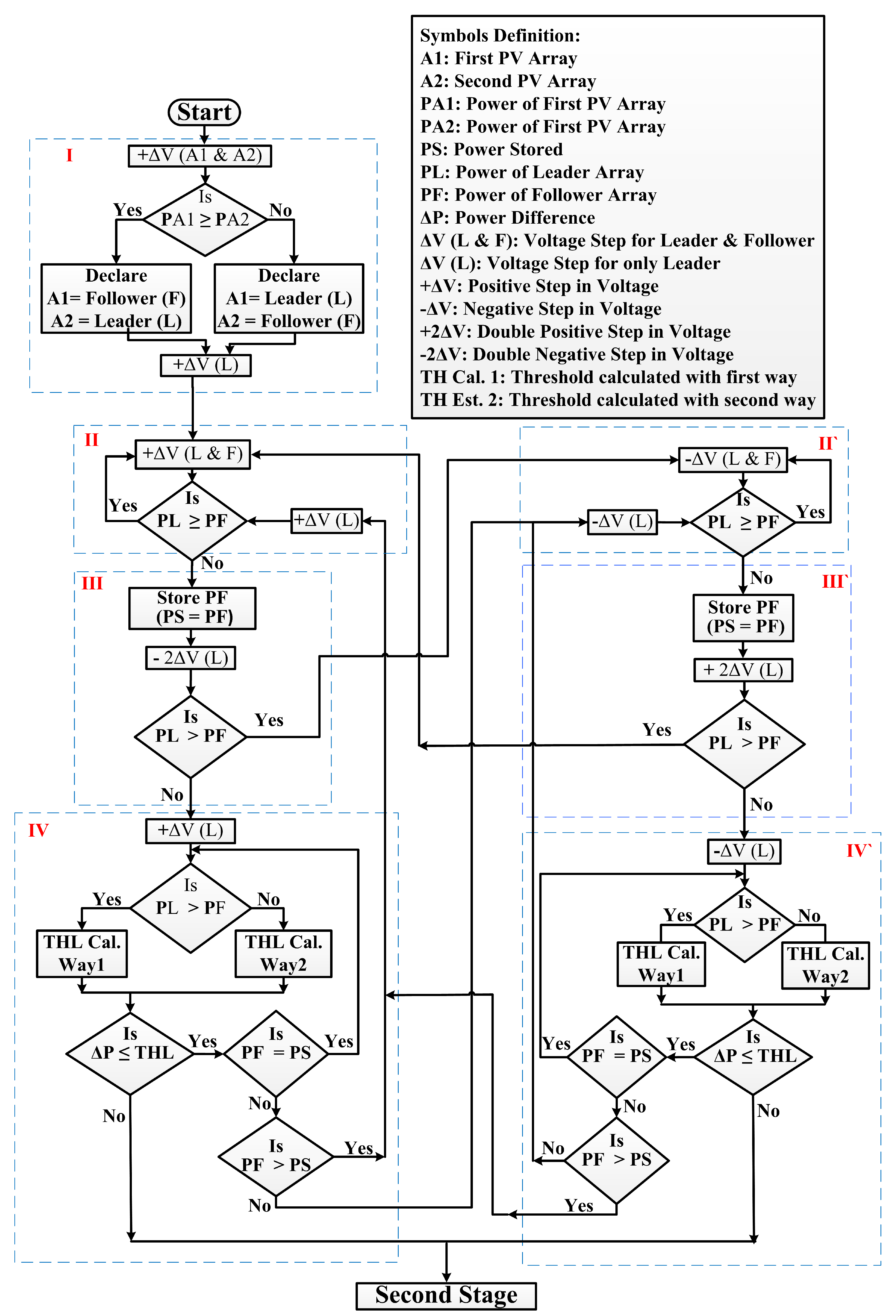
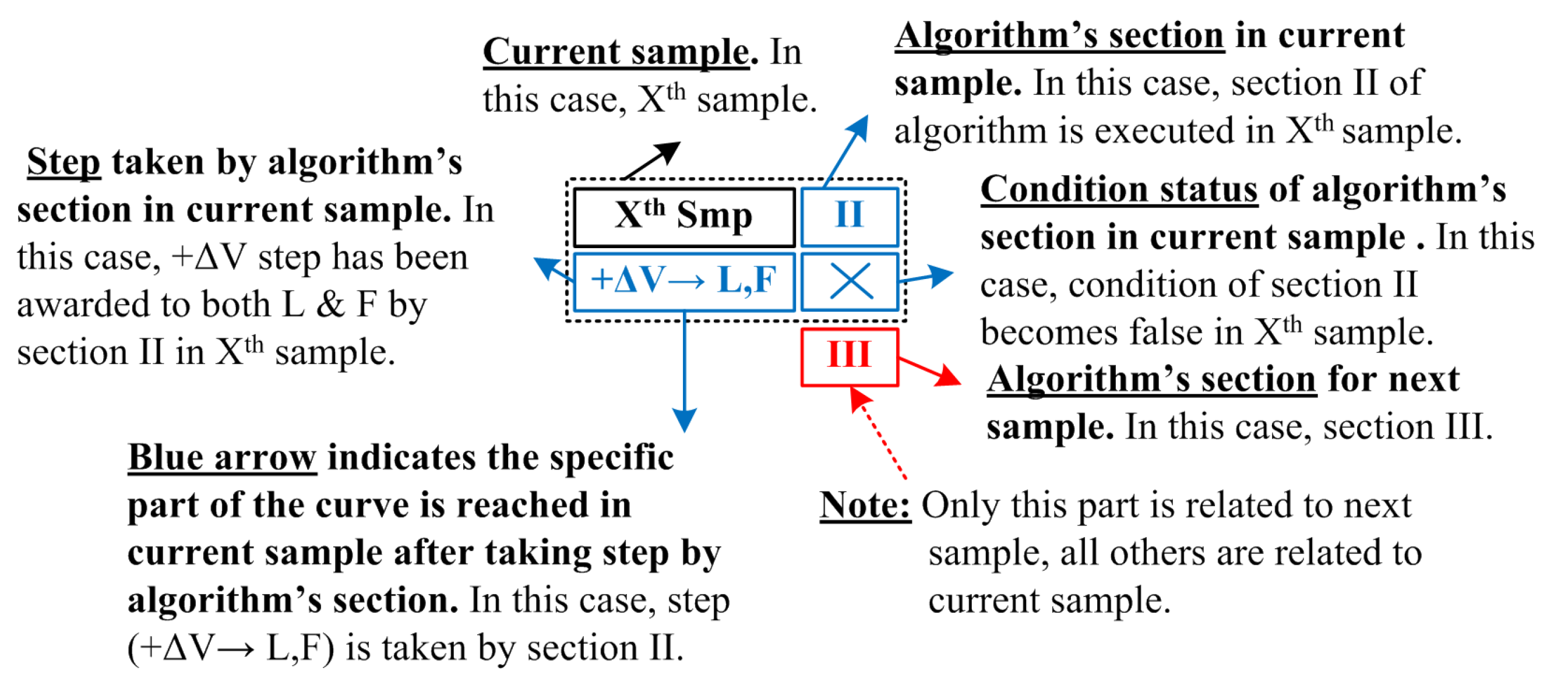
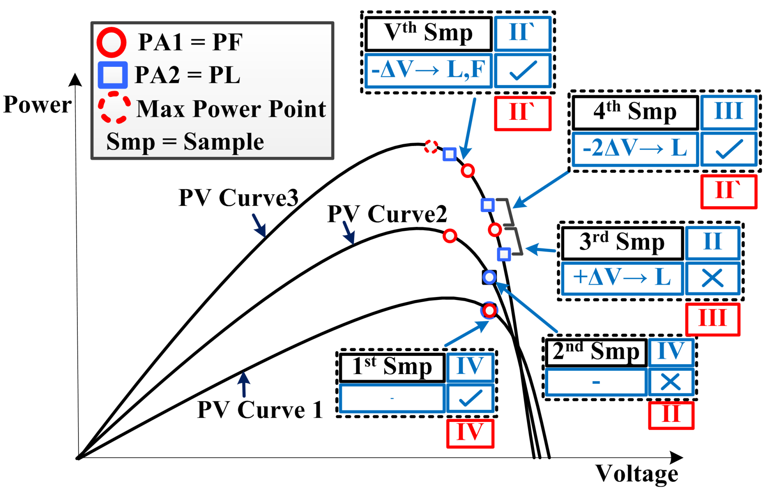
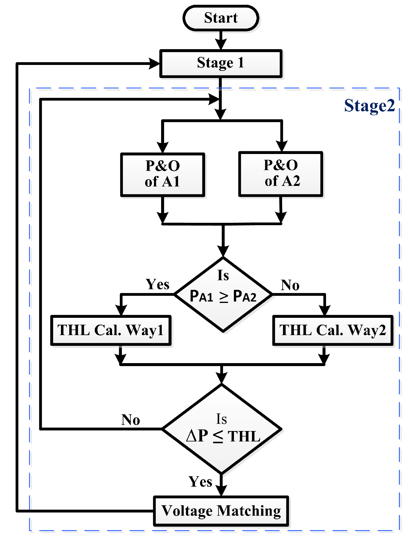
4. Working of Proposed Technique

The proposed technique is based on a two stage operation. The flowchart of stage 1 is shown in Figure 4; the flowchart of stage 2 is shown in the Section 4.2. The detailed explanation of these two stages is given below.

4.1. Stage 1 (Non-Mismatch Conditions)

The flowchart of stage 1 is shown in Figure 4. It is sub-divided into four sections, recognized as I and pairs of II-II’, III-III’ and IV-IV’. Note that the paired sections perform same logic. Moreover, the flowchart is explained for two arrays A1 and A2.

To have a better understanding of the proposed method, consider Figure 5 to understand group notations for graphical analysis. This notation is for each sample to indicate the working of stage I. A new sample is considered after applying a voltage step.

4.1.1. Scenario 1: Uniform Irradiance Condition

Consider the P-V curve of a PV system shown in Figure 6, in which a constant irradiance condition is considered. Further, consider the 1st sample, which indicates stage 1 of the flowchart shown in Figure 4. Section I provides a positive step voltage (+$\Delta$V) to A1 and A2. Let the power of A1 (PA1) be greater than the power of A2 (PA2) so that A1 is declared a follower (F) while A2 a leader (L). In the 2nd sample, +$\Delta$V is awarded to L(A2) only, after which the flowchart enters section II. The third sample is represented as a $K^{th}$ sample in which section II of the algorithm awards +$\Delta$V to both L(A2) and F(A1). Thereafter, the power difference is computed such that, if PL is more than PF, the algorithm applies another +$\Delta$V to L(A2) and F(A1). The algorithm stays in section II unless the power of the follower array exceeds the power of the leader array.

This process continues until the $W^{th}$ sample is reached. Although in the $W^{th}$ sample, PL becomes equal to MPP but the algorithm stays in section II. In the $X^{th}$ sample, as PF is greater than PL, the algorithm enters in section III for the $Y^{th}$ sample. Section III is an indication that the MPP region is reached and therefore the algorithm stores the power of F by making ‘PS = PF’. At this point, it is feasible to stop the follower. Note that, by using the conventional $P\&O$, this is not possible. During the $Y^{th}$ sample, section III applies a double opposite step to L(A2) only. This is to confirm that MPP is not shifted on the left side due to weather variation. If the PL is greater than PF, then the system moves to section II’, otherwise it enters the stage IV for the next sample. In the $Z^{th}$ sample, Section IV applies +$\Delta$V to L(A2) only. Consequently, both L(A2) and F(A1) reach the desired MPP. Moreover, in Section IV, as both $L\&F$ are stable, the power difference $\Delta P$ and the threshold limit (THL) are calculated either through way 1 or way 2. The THL calculation is explained in the next section. For the non-mismatch condition, both arrays exhibit the same behavior, thereby the threshold condition remains valid, thus eliminating the need to check or store PA1 and PA2. Any change in the weather conditions makes the PF = PS false, which forces the algorithm to move back to some other sections. In case the two arrays become different due to mismatch effects, then the threshold limit condition, that is, $\Delta P\le THL$ becomes false, which forces the algorithm to enter stage 2.

4.1.2. Scenario 2: Varying Weather Condition

In Figure 7, scenario 2 is presented to showcase the working of stage 1 under increasing irradiance and temperature. Consider that, in the 1st sample, P-V curve1 is active and both $L\&F$ are stable in section IV and therefore no step is applied to $L\&F$. In the 2nd sample, the irradiance and temperature increase; consequently, the system moves to P-V curve 2. This violates the condition “PF = PS”; also, as PF becomes greater, the algorithm enters section II for the next sample. In the 3rd sample, again the weather changes so the system shifts to P-V curve 3. In this sample, section II gives $\Delta P$ to L(A2) only, and it is clear that the algorithm takes a wrong step. So, in the 4th sample, the algorithm executes section III, which gives the 2$\Delta P$ step to L(A2), thus compensating for the wrong direction. As in the 4th sample, the condition becomes true so the algorithm then enters section II’. Thereby, continue with section II‘ until MPP is reached.

4.2. Stage 2 (Mismatch Conditions)

A flowchart of stage 2 is shown in Figure 8. It is a modified $P\&O$ method to handle two PV arrays simultaneously. Other exceptions are the threshold and voltage matching mechanisms. In each cycle, the proposed technique executes the $P\&O$ algorithm on each array separately. Before executing the next cycle, the output power of two arrays is calculated and compared. Thereafter, the threshold mechanism is applied based on the expressions given in Equations (1)–(4). The cycle is repeated until the power difference between array 1 and array 2 comes within the threshold limit.

5. Concept Validation

Simulation Setup

The Matlab/Simulink model of PV arrays proposed by [31] is used for simulations. The datasheet of the PV module is shown in

Table 2. Specifications of Kyocera-KC200GT at STC.

Parameters	Value
$I_{sc}\left(A\right)$	8.21
$V_{oc}\left(V\right)$	32.9
$I_m\left(A\right)$	7.61
$V_m\left(V\right)$	26.3
$P_m\left(W\right)$	200
$K_v(V/K)$	−0.123
$K_i(A/K)$	0.0032
$N_s$	54

. For a level playing ground field, two equal sized PV arrays are used.

The simulation setup is shown in Figure 9. Each array produces 4 kW power through two strings of 10 series connected modules. With two arrays, the net output power of this system is 8 kW at STC. Moreover, each PV array is connected to a load (battery) through a dc-dc boost converter. The input capacitor ($C_{in}$) and output capacitor ($C_{out}$) for both converters are set at 300 $\mathsf{\mu }$F and 0.001 $\mathsf{\mu }$F, respectively, while inductor (L) for both converters is set at 10 mH. The switching frequency for boost converters is settled at 5 kHz. The MPPT controller controls the duty cycle (D) of both boost converters through the PWM unit. For benchmarking the proposed MPPT, two algorithms are compared in simulations which are: (1) dual array based incremental conductance (D-IC) [6,22,23] and (2) conventional $P\&O$ running on individual arrays (Conv. $P\&O$). For each algorithm, the MPPT controller changes D with a resolution of 1%, consequently, each algorithm has a voltage step (+/−$\Delta$V) of approximately 6 V. The sampling rate of the PV system is set at 10 ms. For the D-IC algorithm, the voltage difference between two PV arrays is set at approximately 1.5 V while the accuracy of the power difference ($\Delta$P = 0) between two arrays is set between −1 W to 1 W. Because of ripples, a tolerance of 1 W is given to the D-IC algorithm.

6. Results and Discussion

Simulations are divided into three categories of weather conditions. The performance of each algorithm is then analyzed under these categories. All three algorithms are tested on five different weather conditions. The response of each algorithm is evaluated case by case. Finally, their performance is summarized.

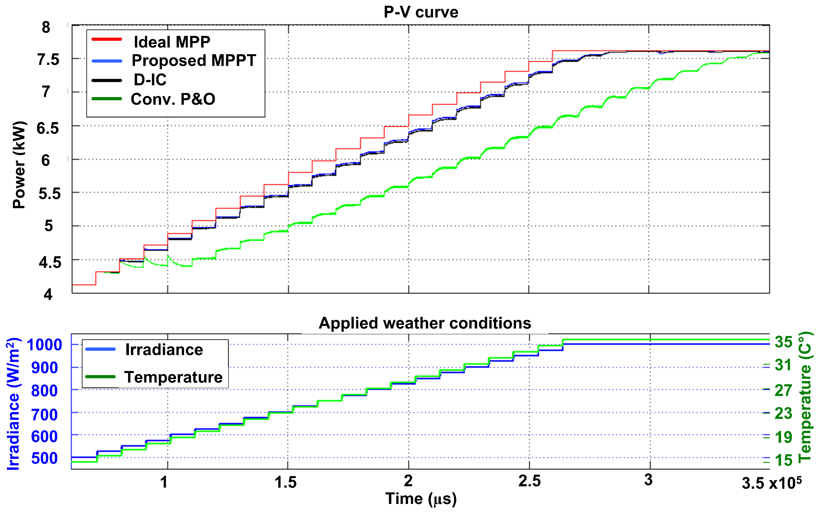
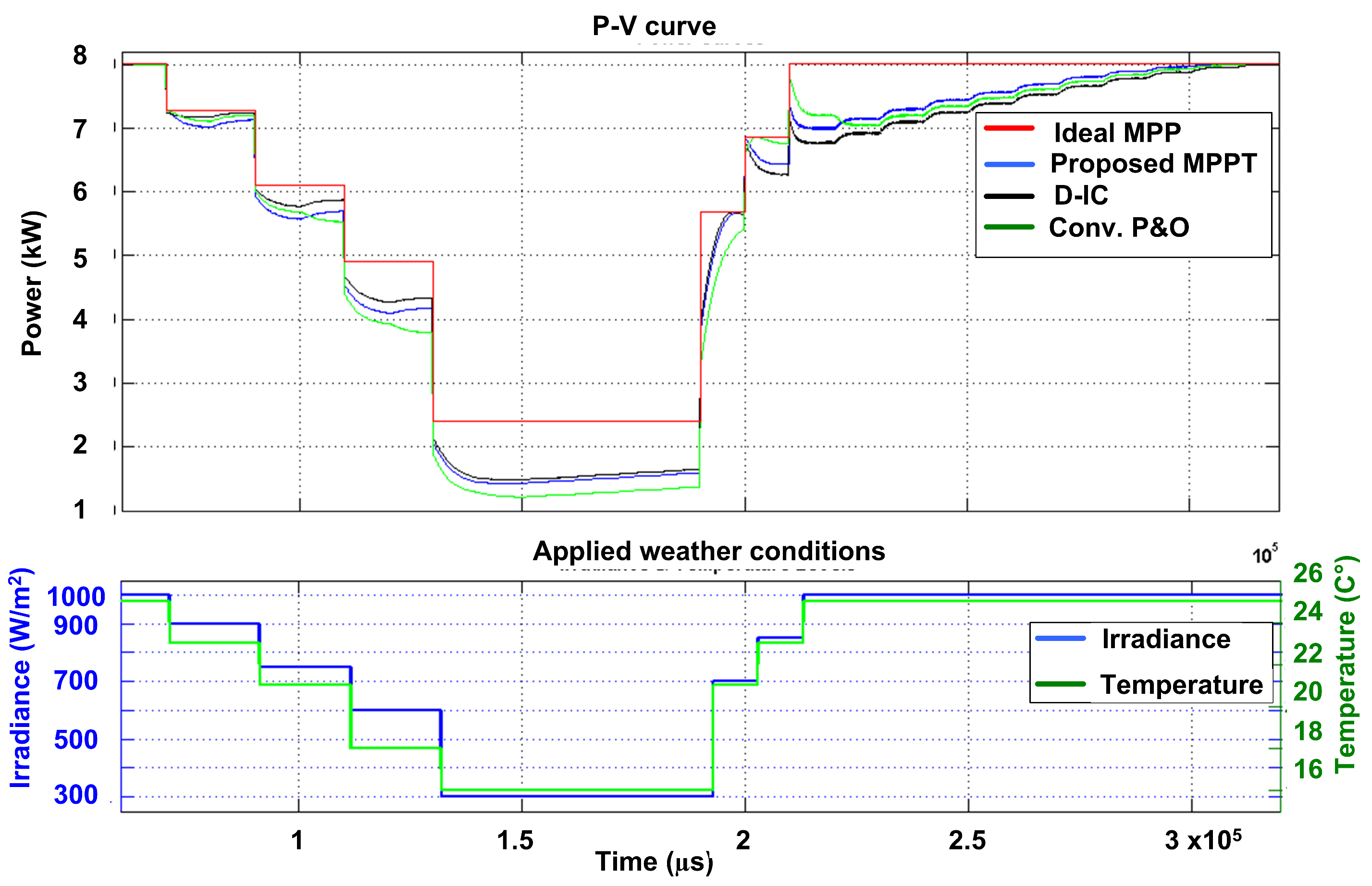
6.1. Case 1: Step Increment in Weather Conditions

The environmental condition is initiated at 500$\frac{W}{m^2}$–15 ${}^{\circ }$C. A step change in irradiance and temperature is applied at a step increment of 25$\frac{W}{m^2}$ at 1 ${}^{\circ }$C per sample until the weather conditions equal 1000$\frac{W}{m^2}$–and 35 ${}^{\circ }$C as shown in Figure 10. The power outcome of three algorithms is also shown in Figure 10. As evident from the results, the proposed MPPT method responded well under the applied weather conditions compared to the D-IC and $P\&O$.

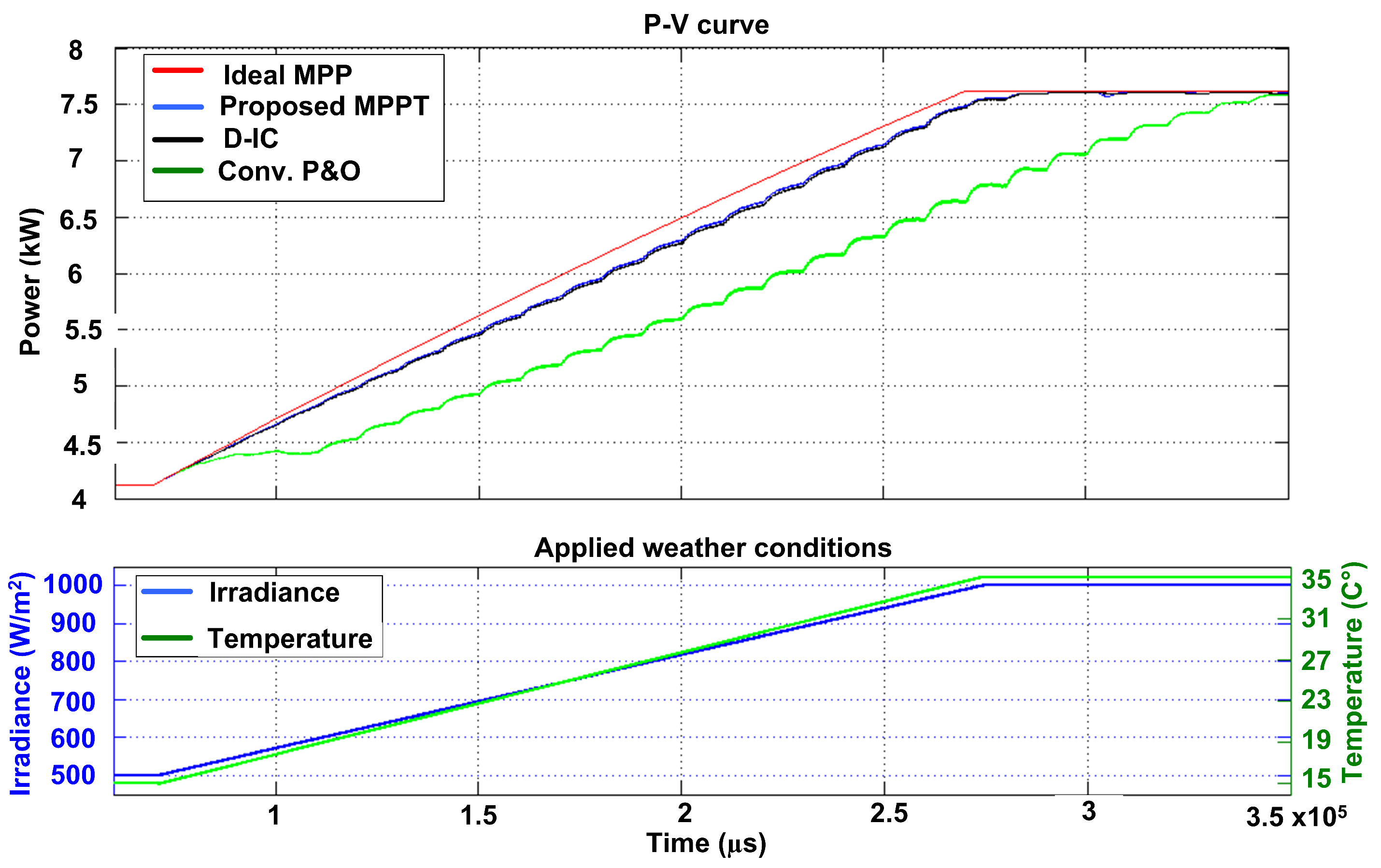
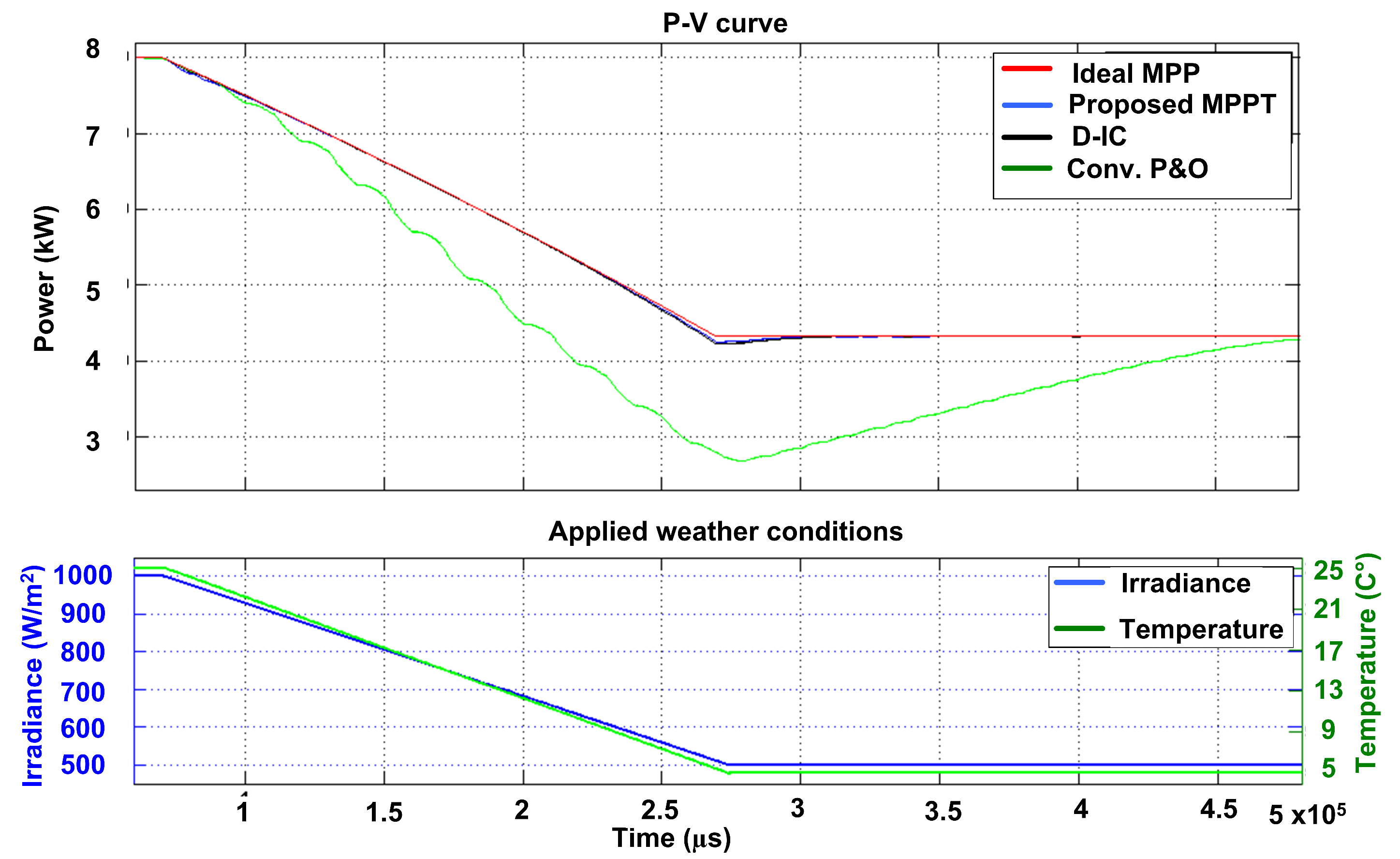
6.2. Case 2: Ramp Increment in Weather Conditions

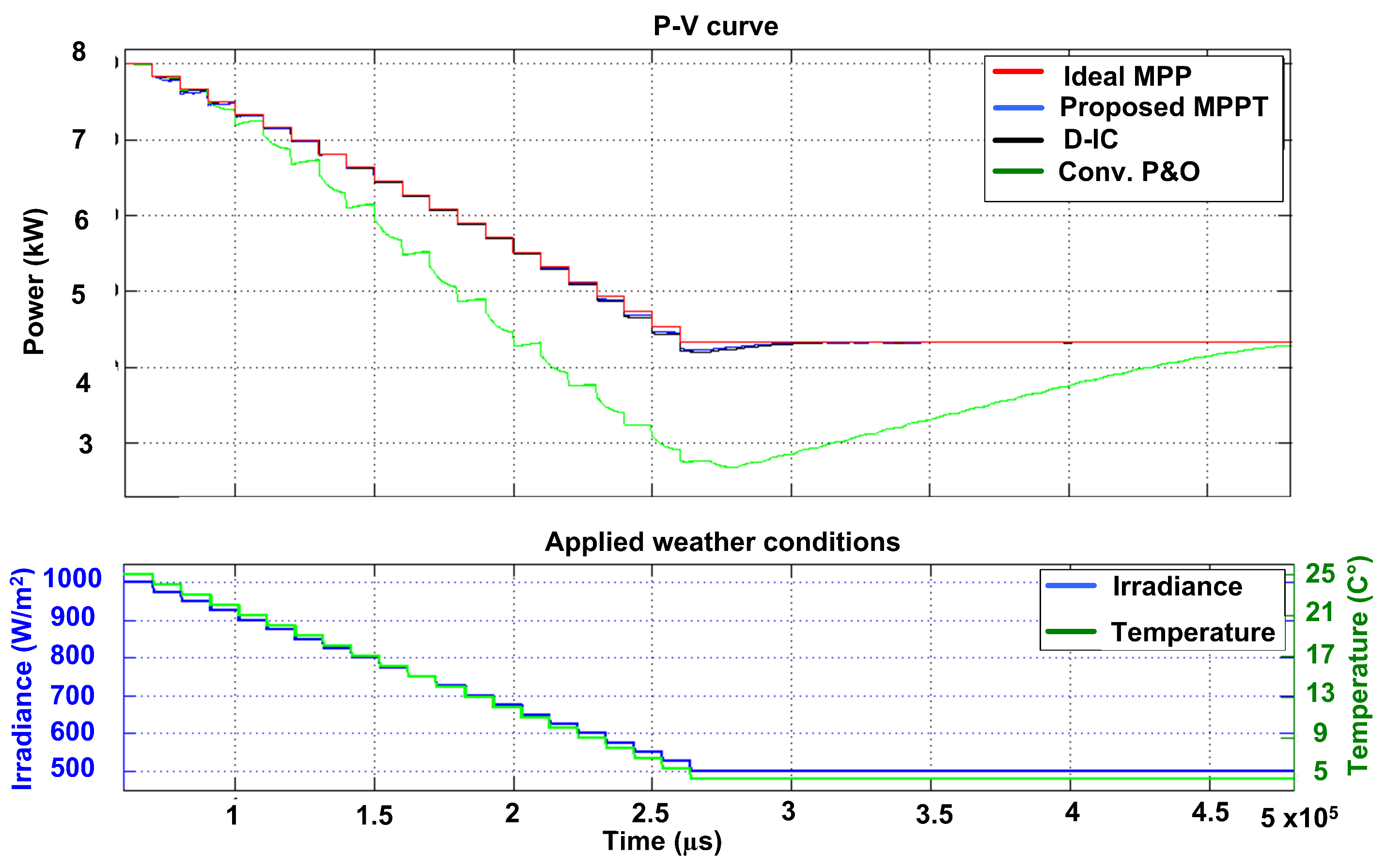
Case 1 weather conditions in the ramp case are applied. The irradiance–temperature is subjected to change linearly at a rate of 25$\frac{W}{m^2}$ at 1 ${}^{\circ }$C per sample as shown in Figure 11. It is visible that $P\&O$ struggles in attaining MPPT followed by D-IC MPPT. However, the proposed MPPT has shown a superior performance compared to both algorithms.

6.3. Case 3

All three algorithms are first settled at the environment of 1000$\frac{W}{m^2}$–25 ${}^{\circ }$C. Thereafter, the irradiance and temperature are varied at a step decrement of 25$\frac{W}{m^2}$–1 ${}^{\circ }$C per sample up to 500$\frac{W}{m^2}$–5 ${}^{\circ }$C as shown in Figure 12. It can be seen that the proposed method works best while the D-IC method also works well. However, the $P\&O$ struggle becomes much more prominent and its performance degrades further under these conditions.

6.4. Case 4

In this case, irradiance and temperature are subjected to decay linearly at a rate of 25$\frac{W}{m^2}$ at 1 ${}^{\circ }$C as shown in Figure 13. This test again testifies the performance of the proposed MPPT, which outperforms the $P\&O$ and D-IC as displayed in Figure 13.

6.5. Case 5

A cloud passing scenario is realized in this case. First, weather is settled at 1000$\frac{W}{m^2}$ at 25 ${}^{\circ }$C. Thereafter, it is subjected to a sequence of step decrement: first, 900$\frac{W}{m^2}$ at 23 ${}^{\circ }$C for two samples, second 750$\frac{W}{m^2}$ at 21 ${}^{\circ }$C for two samples, third 600$\frac{W}{m^2}$ at 18 ${}^{\circ }$C for two samples and finally 300$\frac{W}{m^2}$ at 16 ${}^{\circ }$C for six samples. After these decaying sequences, weather conditions return back to 1000$\frac{W}{m^2}$ at 25 ${}^{\circ }$C following a step rise to 700$\frac{W}{m^2}$ at 21 ${}^{\circ }$C for one sample and 850$\frac{W}{m^2}$ at 23 ${}^{\circ }$C for another sample. These weather conditions are visualized in Figure 14. This test validates the effectiveness of the proposed method compared to the D-IC and $P\&O$.

6.6. Summary

The efficiency of algorithms under five cases is summarized in

Table 3. Efficiency table of algorithms under five dynamic weather cases.

Case	Type	Measurement Period	Efficiency (%) proposed MPPT	Efficiency (%) D-IC	Efficiency (%) Conv. $\mathit{P}\&\mathit{O}$
1	Step rise	70−350 ms	98.21	97.98	90.91
2	Ramp rise	70−350 ms	98.59	98.37	90.81
3	Step decay	70−480 ms	99.66	99.6	84.46
4	Ramp decay	70−480 ms	99.78	99.74	84.97
5	Cloud pass	70−320 ms	91.31	91.06	89.95

. Efficiency is calculated from the point when weather conditions started to change to the point when the slowest algorithm reaches MPP after conditions settle down. As in case 1, efficiency is evaluated between 70 ms to 350 ms. It is because although proposed MPPT and D-IC reaches MPP quite early before 350 ms but $P\&O$ reaches MPP at 350 ms after it is settled. Analyzing Table 3, it is proved that the proposed MPPT overcomes the problems of conventional $P\&O$ under fast varying weather conditions. It not only enhanced the efficiency but is able to attain greater efficiency than D-IC.

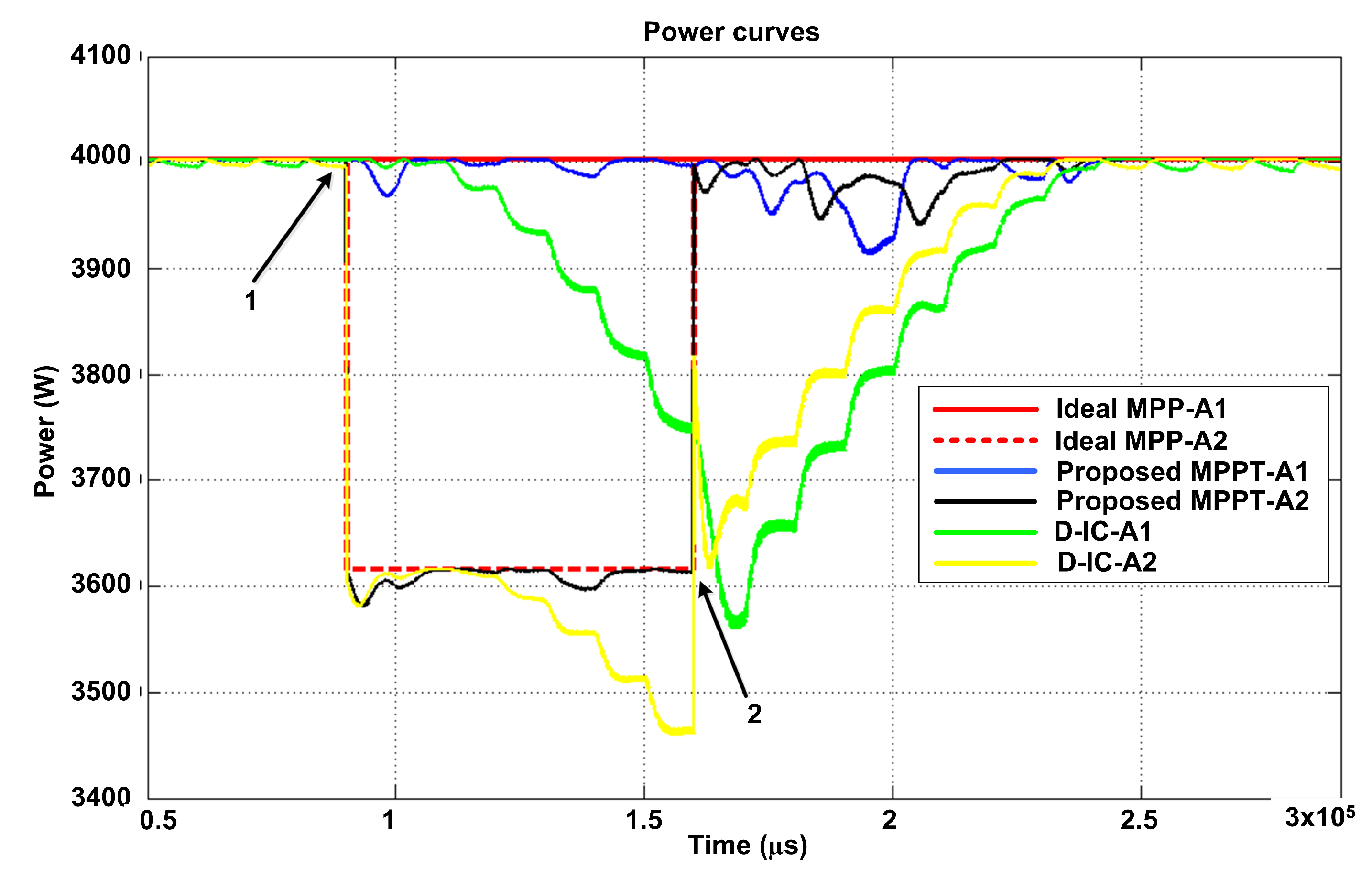
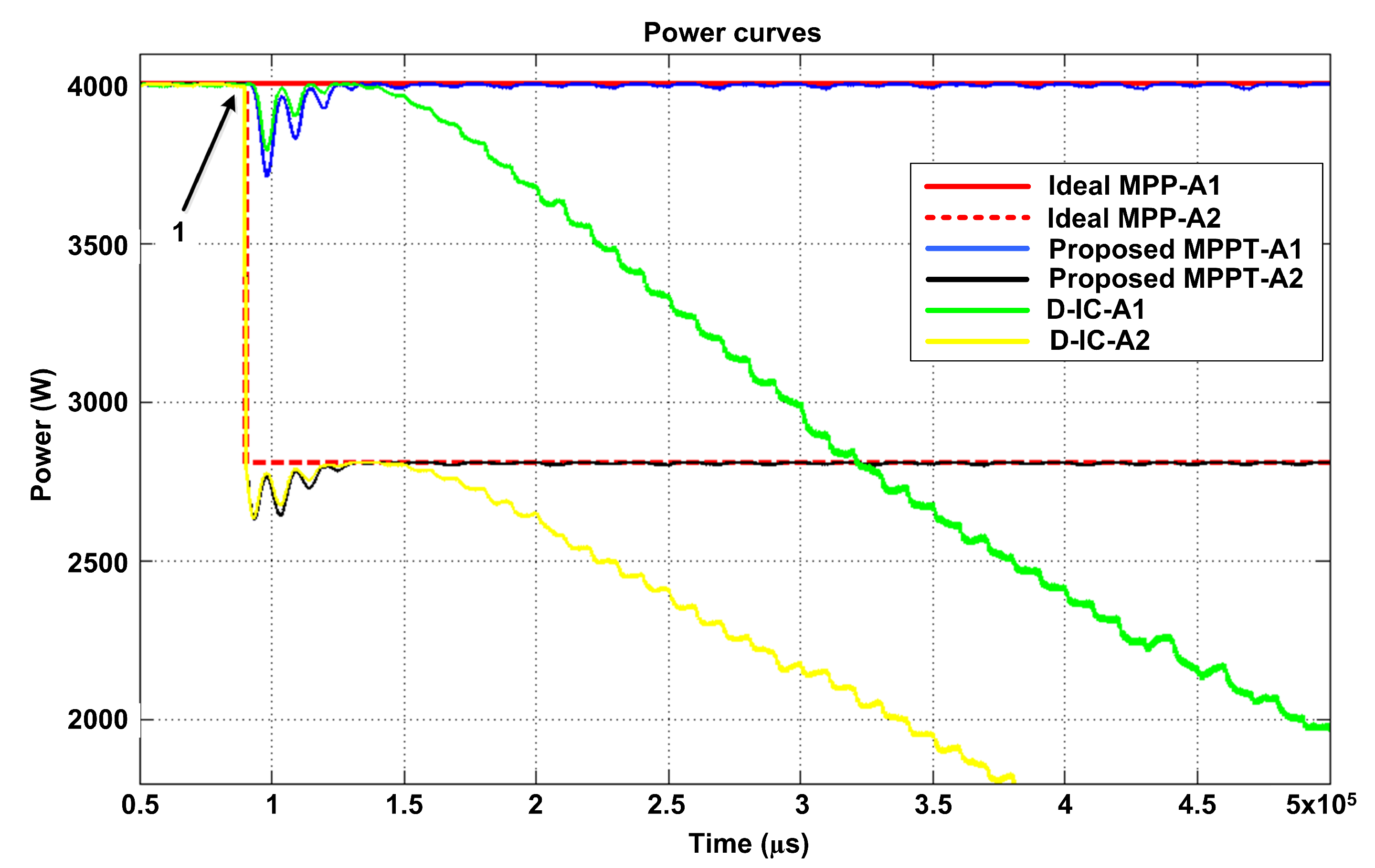
6.7. Partial Shading

The proposed method is also benchmarked against two partial shading cases. In this category, the algorithm responses of both PV arrays (A1 & A2) are shown separately. Note that, during partial shading, the proposed MPPT operates in stage 2.

6.7.1. Case 1

In this case, initially both A1 & A2 are given the weather conditions of 1000$\frac{W}{m^2}$ at 25 ${}^{\circ }$C. At point 1 (shown with an arrow), A2 is assumed to be shaded such that the weather condition becomes 900 $\frac{W}{m^2}$ at 24 ${}^{\circ }$C. The condition persists until point 2 (shown with an arrow), at which both arrays once again operate under same weather conditions of 1000$\frac{W}{m^2}$ at 25 ${}^{\circ }$C. It can be seen from Figure 15 that the proposed technique and D-IC struggles on two occasions: (1) when both arrays had different conditions at arrow-1 position and (2) when both arrays again had the same conditions at the arrow-2 position. Under these two occasions, the proposed technique quickly responded to the conditions and was able to retain MPP at a rate much faster rate than D-IC. It should be further noted that the proposed MPPT enters stage 2 at the arrow-1 position, while it returns back to stage 1 at the arrow-2 position when both arrays had the same conditions. This shows the ability of the algorithm to handle these partial shading situations effectively.

6.7.2. Case 2

In this case, arrays A1 & A2 are first operated at 1000$\frac{W}{m^2}$ at $-25$${}^{\circ }$C. Then, at point 1, A2 is partially shaded at 700$\frac{W}{m^2}$ at 23 ${}^{\circ }$C. It is evident from Figure 16 that, if two arrays have mismatch conditions for quite a long time then it heavily impacts the performance of D-IC. In fact, it is a complete failure of D-IC because of its inherent deficiency of not handling the partial shading conditions. While the proposed algorithm is able to deal with these conditions efficiently and is able to track MPP well, maintaining the advantage of DPV systems under partial shading conditions.

7. Conclusions

In this paper, a new two stage MPPT technique is proposed for DPV plants. Stage 1 is designed for the DPV plant under uniform weather conditions. While stage 2 ensures that the DPV plant maintains its advantage over the centralized PV plant under partial shading conditions, stage 1 adopts an intelligent leader–follower communication between two arrays/modules. A new graphical analysis has been presented to verify the effectiveness of stage 1. The proposed MPPT is a benchmark with the performance of a conventional perturb and observe MPPT and distributed incremental conductance under dynamic and partial shading conditions. Simulation analysis revealed that the proposed MPPT technique overcomes the issues related to conventional MPPT methods. It is further illustrated through simulation results that dual modules/arrays based MPPT techniques cannot perform under the mismatch conditions.

References

1. Adeel, M.; Hassan, A.K.; Sher, H.A.; Murtaza, A.F. A grade point average assessment of analytical and numerical methods for parameter extraction of a practical PV device. Renew. Sustain. Energy Rev. 2021, 142, 110826. [Google Scholar] [CrossRef]
2. Ahmad, R.; Murtaza, A.F.; Sher, H.A.; Shami, U.T.; Olalekan, S. An analytical approach to study partial shading effects on PV array supported by literature. Renew. Sustain. Energy Rev. 2017, 74, 721–732. [Google Scholar] [CrossRef]
3. Adinolfi, G.; Femia, N.; Petrone, G.; Spagnuolo, G.; Vitelli, M. Design of dc/dc Converters for DMPPT PV Applications Based on the Concept of Energetic Efficiency. J. Sol. Energy Eng. 2010, 132, 021005. [Google Scholar] [CrossRef]
4. Chao, R.M.; Ko, S.H.; Lin, H.K.; Wang, I.K. Evaluation of a distributed photovoltaic system in grid-connected and standalone applications by different MPPT algorithms. Energies 2018, 11, 1484. [Google Scholar] [CrossRef] [Green Version]
5. Ahmad, R.; Murtaza, A.F.; Sher, H.A. Power tracking techniques for efficient operation of photovoltaic array in solar applications—A review. Renew. Sustain. Energy Rev. 2019, 101, 82–102. [Google Scholar] [CrossRef]
6. Park, J.H.; Ahn, J.Y.; Cho, B.H.; Yu, G.J. Dual-module-based maximum power point tracking control of photovoltaic systems. IEEE Trans. Ind. Electron. 2006, 53, 1036–1047. [Google Scholar] [CrossRef]
7. Femia, N.; Lisi, G.; Petrone, G.; Spagnuolo, G.; Vitelli, M. Distributed maximum power point tracking of photovoltaic arrays: Novel approach and system analysis. IEEE Trans. Ind. Electron. 2008, 55, 2610–2621. [Google Scholar] [CrossRef] [Green Version]
8. Delavaripour, H.; Dehkordi, B.M.; Zarchi, H.A.; Adib, E. Increasing energy capture from partially shaded PV string using differential power processing. IEEE Trans. Ind. Electron. 2018, 66, 7672–7682. [Google Scholar] [CrossRef]
9. Petrone, G.; Spagnuolo, G.; Vitelli, M. An analog technique for distributed MPPT PV applications. IEEE Trans. Ind. Electron. 2011, 59, 4713–4722. [Google Scholar] [CrossRef]
10. Murtaza, A.F.; Sher, H.A.; Chiaberge, M.; Boero, D.; De Giuseppe, M.; Addoweesh, K.E. Comparative analysis of maximum power point tracking techniques for PV applications. In Proceedings of the INMIC, Lahore, Pakistan, 19–20 December 2013; pp. 83–88. [Google Scholar]
11. Petrone, G.; Ramos-Paja, C.A.; Spagnuolo, G.; Vitelli, M. Granular control of photovoltaic arrays by means of a multi-output Maximum Power Point Tracking algorithm. Prog. Photovolt. Res. Appl. 2013, 21, 918–932. [Google Scholar] [CrossRef]
12. Miyatake, M.; Veerachary, M.; Toriumi, F.; Fujii, N.; Ko, H. Maximum power point tracking of multiple photovoltaic arrays: A PSO approach. IEEE Trans. Aerosp. Electron. Syst. 2011, 47, 367–380. [Google Scholar] [CrossRef]
13. Renaudineau, H.; Donatantonio, F.; Fontchastagner, J.; Petrone, G.; Spagnuolo, G.; Martin, J.P.; Pierfederici, S. A PSO-based global MPPT technique for distributed PV power generation. IEEE Trans. Ind. Electron. 2014, 62, 1047–1058. [Google Scholar] [CrossRef]
14. Sher, H.A.; Murtaza, A.F.; Noman, A.; Addoweesh, K.E.; Al-Haddad, K.; Chiaberge, M. A new sensorless hybrid MPPT algorithm based on fractional short-circuit current measurement and P&O MPPT. IEEE Trans. Sustain. Energy 2015, 6, 1426–1434. [Google Scholar]
15. López-Erauskin, R.; González, A.; Petrone, G.; Spagnuolo, G.; Gyselinck, J. Multi-Variable Perturb and Observe Algorithm for Grid-Tied PV Systems With Joint Central and Distributed MPPT Configuration. IEEE Trans. Sustain. Energy 2020, 12, 360–367. [Google Scholar] [CrossRef]
16. Sher, H.A.; Murtaza, A.F.; Addoweesh, K.E.; Chiaberge, M. A two stage hybrid maximum power point tracking technique for photovoltaic applications. In Proceedings of the 2014 IEEE PES General Meeting | Conference & Exposition, National Harbor, MD, USA, 27–31 July 2014; pp. 1–5. [Google Scholar]
17. Petrone, G.; Spagnuolo, G.; Teodorescu, R.; Veerachary, M.; Vitelli, M. Reliability issues in photovoltaic power processing systems. IEEE Trans. Ind. Electron. 2008, 55, 2569–2580. [Google Scholar] [CrossRef]
18. Kollimalla, S.K.; Mishra, M.K. Variable perturbation size adaptive P&O MPPT algorithm for sudden changes in irradiance. IEEE Trans. Sustain. Energy 2014, 5, 718–728. [Google Scholar]
19. Jiang, Y.; Qahouq, J.A.A.; Haskew, T.A. Adaptive step size with adaptive-perturbation-frequency digital MPPT controller for a single-sensor photovoltaic solar system. IEEE Trans. Power Electron. 2012, 28, 3195–3205. [Google Scholar] [CrossRef]
20. Killi, M.; Samanta, S. Modified perturb and observe MPPT algorithm for drift avoidance in photovoltaic systems. IEEE Trans. Ind. Electron. 2015, 62, 5549–5559. [Google Scholar] [CrossRef]
21. Ahmed, J.; Salam, Z. A modified P&O maximum power point tracking method with reduced steady-state oscillation and improved tracking efficiency. IEEE Trans. Sustain. Energy 2016, 7, 1506–1515. [Google Scholar]
22. Behera, T.K.; Behera, M.K.; Nayak, N. Spider monkey based improve P&O MPPT controller for photovoltaic generation system. In Proceedings of the 2018 Technologies for Smart-City Energy Security and Power (ICSESP), Bhubaneswar, India, 28–30 March 2018; pp. 1–6. [Google Scholar]
23. Murtaza, A.F.; Sher, H.A.; Chiaberge, M.; Boero, D.; De Giuseppe, M.; Addoweesh, K.E. A novel hybrid MPPT technique for solar PV applications using perturb & observe and fractional open circuit voltage techniques. In Proceedings of the 15th International Conference MECHATRONIKA, Prague, Czech Republic, 5–7 December 2012; pp. 1–8. [Google Scholar]
24. Sher, H.A.; Rizvi, A.A.; Addoweesh, K.E.; Al-Haddad, K. A single-stage stand-alone photovoltaic energy system with high tracking efficiency. IEEE Trans. Sustain. Energy 2016, 8, 755–762. [Google Scholar] [CrossRef]
25. Sher, H.A.; Addoweesh, K.E.; Al-Haddad, K. An efficient and cost-effective hybrid MPPT method for a photovoltaic flyback microinverter. IEEE Trans. Sustain. Energy 2017, 9, 1137–1144. [Google Scholar] [CrossRef]
26. Han, C.; Lee, H. Investigation and modeling of long-term mismatch loss of photovoltaic array. Renew. Energy 2018, 121, 521–527. [Google Scholar] [CrossRef]
27. Grandi, G.; Ostojic, D. Dual-inverter-based MPPT algorithm for grid-connected photovoltaic systems. In Proceedings of the 2009 International Conference on Clean Electrical Power, Capri, Italy, 9–11 June 2009; pp. 393–398. [Google Scholar]
28. Grandi, G.; Rossi, C.; Fantini, G. Modular photovoltaic generation systems based on a dual-panel MPPT algorithm. In Proceedings of the 2007 IEEE International Symposium on Industrial Electronics, Vigo, Spain, 4–7 June 2007; pp. 2432–2436. [Google Scholar]
29. Chamberlin, C.E.; Lehman, P.; Zoellick, J.; Pauletto, G. Effects of mismatch losses in photovoltaic arrays. Sol. Energy 1995, 54, 165–171. [Google Scholar] [CrossRef]
30. Spertino, F.; Akilimali, J.S. Are Manufacturing IV Mismatch and Reverse Currents Key Factors in Large Photovoltaic Arrays? IEEE Trans. Ind. Electron. 2009, 56, 4520–4531. [Google Scholar] [CrossRef] [Green Version]
31. Villalva, M.G.; Gazoli, J.R.; Ruppert Filho, E. Comprehensive approach to modeling and simulation of photovoltaic arrays. IEEE Trans. Power Electron. 2009, 24, 1198–1208. [Google Scholar] [CrossRef]
Figure 1. Distributed PV plant with MPPT mechanism.
Energies 14 06996 g001
Figure 2. Centralized PV plant with MPPT mechanism.
Energies 14 06996 g002
Figure 3. Basic scheme of proposed MPPT.
Energies 14 06996 g003
Figure 4. Flowchart of Stage 1 of the proposed MPPT.
Energies 14 06996 g004
Figure 5. Group notations understanding.
Energies 14 06996 g005
Figure 6. Scenario 1: Graphical analysis of proposed technique under uniform irradiance condition.
Energies 14 06996 g006
Figure 7. Scenario 2: Graphical analysis of the proposed technique under varying weather conditions.
Energies 14 06996 g007
Figure 8. Flowchart of stage 2.
Energies 14 06996 g008
Figure 9. Simulation setup.
Energies 14 06996 g009
Figure 10. Case 1: Response of three algorithms against step increment in weather conditions.
Energies 14 06996 g010
Figure 11. Case 2: Response of three algorithms against linear increment in weather conditions.
Energies 14 06996 g011
Figure 12. Case 3: Response of three algorithms against step decrement in weather conditions.
Energies 14 06996 g012
Figure 13. Case 4: Response of three algorithms under linear decay in weather conditions.
Energies 14 06996 g013
Figure 14. Case 5: Response of three algorithms under cloud passing.
Energies 14 06996 g014
Figure 15. Partial Shading Case 1: Response of algorithms.
Energies 14 06996 g015
Figure 16. Partial Shading Case 2: Response of algorithms.
Energies 14 06996 g016