Abstract
The problem of transport is a special type of mathematical programming designed to search for the optimal distribution network, taking into account the set of suppliers and the set of recipients. This article proposes an innovative approach to solving the transportation problem and devises source codes in GNU Octave (version 3.4.3) to avoid the necessity of carrying out enormous calculations in traditional methods and to minimize transportation costs, fuel consumption, and CO emission. The paper presents a numerical example of a solution to the transportation problem using: the northwest corner, the least cost in the matrix, the row minimum, and Vogel’s Approximation Methods (VAM). The joint use of mathematical programming and optimization was applicable to real conditions. The transport was carried out with medium load trucks. Both suppliers and recipients of materials were located geographically within the territory of the Republic of Poland. The presented model was supported by a numerical example with interpretation and visualization of the obtained results. The implementation of the proposed solution enables the user to develop an optimal transport plan for individually defined criteria.
1. Introduction
It is particularly important to be able to optimize road transport operations and to use economic theories to solve transportation problems. In literature, problems related to the reduction of computational complexity of the transportation algorithms using, e.g., the C++ programming language or the Matlab environment, were repeatedly addressed. However, it must be acknowledged that they require the user to have a thorough knowledge of the functions available and be proficient in their use. A GNU Octave also allows to use programming techniques, generate new user functions, or perform complex numerical calculations. So far, determining the optimal solution of the transportation problem using programming in GNU Octave was not studied. Therefore, the aim of this article was to devise source codes in free GNU Octave (version 3.4.3) environment to minimize transportation costs, fuel consumption, and CO emission.
1.1. Transportation of Materials in Supply Network
From a mathematical point of view, transportation problems have a wide range of applications in logistic systems [1]. Service network design problems arise wherever there is a need to determine cost minimizing routes and schedules, given the constraints on resource availability and level of service [2]. In [3], an agent-based simulation model studying the evolution of a coalition over time taking into account various trust-related issues was developed. Providing efficient distribution systems for services became a challenging issue for logistics companies. Mixed delivery approach, which combines attended home delivery (AHD) and shared delivery locations (SDL) usage in an innovative way, was proposed in [4]. In real-life situations, the traditional transportation problems deals with issues such as transportation costs, selection of delivery routes, selection of production places, or reduction of carbon emissions [5,6,7,8]. Indeed, it is necessary to plan the transportation of materials within the supply network rationally and optimally [9]. In the case of a balanced transportation problem, the balance between supply and demand is assumed. Due to the practical nature of the problem and the effectiveness of the methodology, the transportation algorithm is often used [10,11,12]. The paper [13] is concerned with the design of efficient exact and heuristic algorithms for addressing a bilevel network pricing problem, where demand is a nonlinear function of travel cost. Metaheuristic approach for solving transportation problem with fixed costs associated to the routes was presented in [14]. In distribution networks, rational transport management also requires organizational efforts related to the dynamics and type of tasks [15,16,17]. The costs of transport tasks should be optimized using methods and tools used not only in commercial solutions [18,19,20]. The literature often addresses cases aimed at developing the most effective method of solving transportation problems according to time or cost, while using the available IT tools [21,22]. In the paper [23] one of the first basic transportation problem was formalized, which was then further developed in [24], and then expanded even more in [25] by using the simplex method. There are a number of methods leading to a basic feasible solution to the transportation problem. The most common methods used to support the decision making process are: the northwest corner method, the row minimum method, the least cost in the matrix, and VAM method (Vogel’s Approximation Method).
1.2. Modifications of Existing Methods
An innovative method of solving the transport problem based on the northwest corner method is described in the paper [26]. The authors, by deliberately modifying the cost matrix before applying the northwest corner method, proved that the proposed solution positively influences the effectiveness of the method by reducing the number of iterations performed. In [27], an analysis was made of the number of steps necessary to determine the optimal transport problem using the northwest corner method, the minimum cost method, and the VAM method. The subject of the research were transport cost matrices with dimensions of , while the values of supply and demand were generated in a random way from a set of numbers from 5 to 50,000. On the basis of the obtained results, it was found that the number of iterations required to obtain an optimal solution when using the northwest corner method in the case of matrices with dimensions of is as much as six-times higher than when using the minimum cost method or the VAM method. In [28], an alternative method of solving the balanced transport problem, so-called TCM (Tuncay Can Approximation Method), based on the geometric average of transportation costs, was used. A novel method called KSAM (Karagul–Sahin Approximation Method) used to find an initial solution to the transportation problem was proposed in [29]. The solutions obtained by KSAM were as good as the solutions obtained with the VAM method and as fast as the northwest corner method. In [30] the MOMC method (Maximum Supply with Minimum Cost) was used and the results were compared with three classical methods, i.e., the northwest corner method, the minimum cost method and the VAM method. The MOMC method provides a solution that minimizes the objective function and offers a computational advantage in the form of faster data processing and reduced memory usage. The article [31] analyses the VAM method and proposes how to improve it by using the total alternative cost matrix and alternative allocation costs. Both parametric and nonparametric statistical tests available in the MINITAB-15 statistical package were used in the calculations. In [32], the limitations resulting from the use of the Vogel approximation were discussed and an improved LD-VAM algorithm (Logical Development of Vogel’s Approximation Method) providing a lower objective function value than the VAM method was developed. The paper [33] proposes an ATM (Allocation Table Method) method leading to a basic feasible solution with a lower transportation cost than the solution obtained with traditional algorithms.
1.3. Reduction of Computational Complexity Using the C++ Programming Language
In article [34], a new heuristic method called TOC (Total Opportunity-Cost Method) was proposed to determine the basic feasible solution to the transportation problem, and the results obtained were compared with the classical VAM method. In the publication [35], several variants of the VAM method were analyzed taking into account the concept of Total Opportunity-Cost Method (TOC). Based on the calculations carried out, using the programming language Turbo C++, it was found that the classic VAM method combined with the Total Opportunity-Cost method, the so-called VAM-TOC, results in an optimal or close to optimal solution. Implementation of C++ programming language is also described in [36]. Using the JHM method (Juman & Hoque Method), 18 transportation problems were solved, 11 of which were taken from the literature, and 7 were generated at random. The calculations show that the JHM method in as many as 16 problems considered resulted in a minimum transport cost being determined. In [37], the transportation problem was solved using the northwest corner, minimal cost, the row minimum method, the least cost in the matrix, and the VAM methods. The calculations were carried out in two ways, i.e., by using traditional methodology and object-oriented programming. Due to the need to perform a number of iterations leading to the solution of the problem in question, the C++ programming language was used.
1.4. Practical Application of the Matlab Environment in Transportation Problems
In the literature, there are many solutions to the transportation problem that use the Matlab software. In the paper [38], the problem of transport of chemical substances for a pharmaceutical company using the northwest corner method was analyzed. The Matlab software was also used in [39]. Proposed solution based on the Vogel’s Approximation and Modified Distribution Method would ease the computation of different problems, especially when the problem has a larger cost matrix. In [40], the validity of using the Matlab package was proven not only due to the high efficiency of the algorithm used, but also due to the reduction of time necessary to perform the calculations. In addition, the implementation of the proposed procedure makes it possible to solve the traveling salesman problem. The descriptions of algorithms based on the northwest corner method, the minimum cost method, the VAM method, and the MODI method are included in [41]. The proposed approach emphasizes the superiority of computer programming methods over classical analytical methods.
1.5. Sustainable Transport
Considerable attention is paid to minimizing transport costs with strictly defined supply and demand volumes. However, it should be remembered that during the transport process, the values of both supply and demand can vary over time. The transportation costs to develop a new supplier–retailer inventory model, under the condition that the supplier and the retailer have adopted the two-level trade credit policy, were discussed in article [42]. In [43], a model for taking stock costs into account was defined to determine the lower and upper limit of total transportation costs in a situation of changing supply and demand. The calculations were done using the Matlab software (version ). The significance of the impact of demand variability on the minimization of the supply chain costs is discussed in [44]. The work focuses on optimizing the vehicle speed not only to reduce the transportation costs, but also to reduce carbon emissions while taking into account the variability of demand. The Matlab software was also used for the calculations. The paper [45] presented an analysis of the variability of exhaust emissions from conventional, hybrid, and electric vehicles. The possibility of reducing risks in the supply chain and of using the compound Poisson process was proposed as a possible further research direction. A similar subject was addressed in the paper [46], which explained that rational adjustment of vehicle speeds can offer not only financial but also environmental benefits by reducing carbon dioxide emissions.
1.6. Multicriteria Decision Making Processes
The literature also often addresses issues related to the multicriteria decision making process. In the paper [47] the optimal transport and logistics solution was determined, concerning the distribution of home appliance goods from China to warehouses located in Poland, while ensuring the most favorable conditions for both the manufacturing company and the customers. An integral part of the logistic system is the subsystem of movement and transportation, the aim of which is to ensure the timely and efficient movement of personnel, equipment and supplies in crisis situations. Logistics and transportation simulations that can be used to provide insights into potential outcomes of proposed military deployment plans were presented in [48]. The system of transporting military cargo by means of road transport in peacetime is characterized by high stability. During the period of exercises or combat operations, the high pace of operations requires the commanders to make an effort to monitor and continuously modify the supply routes.
Comparison of research contributions between our paper and related articles was presented in Table 1. The use of our code in GNU Octave allows for effective management of vehicles and for determining optimal distribution plan within supply chain. Moreover, an easy adaptation of the source code could be implemented in other linear programming problems.

Table 1.
Comparison of transportation problems in this paper and related articles.
2. Theoretical Backgrounds for Mathematical Model Development
A transportation problem where total supply is equal to aggregated demand is called a balanced transportation problem. Otherwise, it is an unbalanced transportation problem. Every unbalanced transportation problem can be converted to a balanced transportation problem by adding an artificial supplier or recipient [51,52]. The needs of each recipient as well as the resources of each supplier are known. The distribution of the product should be planned so that transportation costs are minimal [49,53]. The notations used to formulate this problem are presented in Table 2.
Table 2.
List of variables.
The transportation problem can be stated mathematically as a linear programming problem. The objective function described in the formula in Equation (1) minimizes the total cost of transportation between suppliers and recipients:
If total demand is equal to aggregated supply then the relationship in Equation (4) can be noted as:
The feasible solution to the transportation problem is the matrix that meets the conditions (2) and (3), while the optimal solution is a feasible solution that minimizes the objective function (1). The matrix is referred to as the basic feasible solution to the transportation problem relative to base set B if:
The variables and are called base and nonbase variables, respectively, in relation to set B. The next steps of the transportation algorithm are shown below:
- 1.
- Determine the base set B and basic feasible solution ,
- 2.
- Determine the zero matrix equivalent to the cost matrix in relation to the base set B,
- 3.
- For one of the unknowns, take any value and :
- (a)
- other unknowns are to be determined by solving the equation system for ,
- (b)
- determine where , .
- 4.
- Check if the matrix is non-negative. If then is the optimal solution. Otherwise, go to step 4.
- 5.
- Determine a new base set and the corresponding basic feasible solution :
- (a)
- designate a node meeting the condition ,
- (b)
- determine the cycle contained in the set . This cycle should be divided into a positive and a negative semicyclical and , where is in the ,
- (c)
- designate a node semi-cyclical meeting the condition ,
- (d)
- assume ,
- (e)
- determine from the formula:
- 6.
- Go to step 2.
The transportation algorithm is presented in the form of a flowchart in Figure 1.
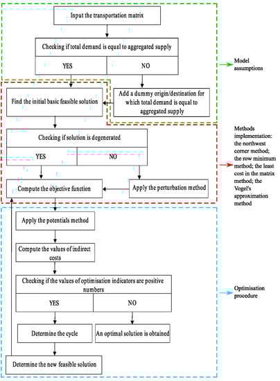
Figure 1.
Flowchart of transportation problem.
3. Methods
3.1. The Northwest Corner Method
The northwest corner method, otherwise known as the upper-left corner method, provides a feasible solution to the considered transportation problem. It does not take into account the transport cost matrix, which may result in high cost of the solution. It consists of subsequent assignment of appropriate values to variables, each time for routes located in the upper left-hand corner of the transport table [54]. It is necessary to come up with a plan for the transport of products from suppliers to recipients in such a way as to ensure minimum transportation costs, with no more than of the product at each point of delivery and no less than of the product at each point of receipt. Transportation takes place along the planned arcs connecting the delivery vertices with the collection vertices (the route from the i-th supplier to the j-th recipient), forming a directed transport network in which the unit transportation costs along each arc are calculated . The solution technique by the northwest corner method is presented as Algorithm 1.
| Algorithm 1 Pseudocode for the Northwest Corner Method | |
| Input: | |
| Output: | |
| while | |
| The first non-zero element is located in the first cell in the northwest corner in matrix X | |
| calculate: | the minimum value among supply or demand for the first cell in the |
| northwest corner | |
| the new value of supply | |
| the new value of demand | |
| if the new value then the remaining cells in this column should | |
| be filled with 0 | |
| endif | |
| if the new value then the remaining cells in this row should | |
| be filled with 0 | |
| endif | |
| the next non-zero elements are located in the next cells in the northwest | |
| corner in matrix X | |
| endwhile | |
| calculate: | total transportation cost for the northwest corner method |
| and the number of basic variables | |
| check: | degeneration of the solution |
| if then solution is degenerated | |
| else solution is non-degenerated | |
| endif | |
Six suppliers located in towns: Zlocieniec, Wesola, Gizycko, Rzeszow, Krakow and Brzeg have 24, 31, 19, 49, 40, 37 loading units, respectively. Eight recipients located geographically in the territory of the Republic of Poland presented in Figure 2 placed an order for 18, 29, 15, 34, 26, 21, 36, 21 loading units respectively. The transportation model was represented by the network shown in Figure 3. The arcs represent the routes linking the destinations and sources.

Figure 2.
Location of suppliers and recipients in territory of Poland.
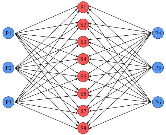
Figure 3.
Network structure of transportation problem.
Taking into account dynamic and necessity to act in crisis situations, analysis of the transportation costs was based on military guidelines and the decision of Chief of the Inspectorate for Armed Forces Support from 19 February 2020. The transport is to be carried out with medium load trucks for which the following unit cost factors were adopted:
- amortisation €,
- maintenance €,
- engine fuels and lubricants €.
The total cost index per exploitation unit is €. Data for numerical problem are presented in Table 3.
Table 3.
Transportation table for numerical example.
At the beginning a table should be prepared with the dimension of m—columns (number of suppliers) and n—lines (number of recipients) taking into account the demand and supply constraints:
To solve the transportation problem using the GNU Octave software (Version 3.4.3/John W. Eaton, Madison, Wl, USA), it is necessary to input the following values: the number of suppliers, the number of recipients and the transportation costs from the i-th supplier to the j-th recipient. In addition, it is necessary to determine demand and supply. Using the northwest corner method, table completion should start with the first cell in the left corner, which corresponds to specific supply and demand values. In the next step, the lower value from among them should be selected and entered in the field corresponding to the first cell of the left corner, and then both supply and demand should be reduced by the value entered. For the first cell, supply assumes a value of 24, while demand is 18. A smaller value is 18, so in the next step, the first cell was supplemented with 18, after which it was subtracted from both supply and demand. At the same time, the software checks which of the demand or supply values is equal zero. If the demand takes a zero value, then the remaining cells in the row under consideration should be completed with zeros. In case the supply would be zeroed, the remaining cells of the column would have to be filled with zeros. Following the same procedure in the next steps, the feasible solution presented in Table 4 was obtained. All nonzero elements are called base elements, while zero elements are called nonbase elements. The solution is degenerated when the number of base elements is meaning . Obtaining an undegenerated solution will make it impossible to check the optimality of the solution using the potential method.
Table 4.
Results of subsequent iterations and feasible solution for northwest corner method.
Transportation cost was computed by using the objective function described in Equation (1). The calculations resulted in a degenerated solution for which the total cost of transport was €165,109.0. Computational source code written in Notepad++ and generated in GNU Octave for finding the basic feasible solution using Northwest Corner Method is given in Appendix A. Lines from 1 to 112 are common to each method. The command window also displays information about the value of the objective function, the number of the base elements, and the degeneration of the received solution.
3.2. The Row Minimum Method
The row minimum method consists of selecting the elements of the C-cost matrix, for which the cost in the first row is minimal. The indicated element corresponds to the value , from which the construction of the base matrix starts. Then, the arcs corresponding to the zero elements of the transformed cost matrix are selected. To determine the initial feasible solution, it is necessary to supplement the X matrix with elements corresponding to arcs with the lowest unit transportation costs in the subsequent rows. Completing the results table using the row minimum method consists of comparing transportation costs and the corresponding values of supply and demand starting from the first row. The solution technique by the row minimum method is presented as Algorithm 2.
The lowest cost in the first row is , with the demand of 18 and supply of 37. In the next step both supply and demand were reduced by 18, resulting in a zero value for demand, as a consequence the remaining cells of the first row were supplemented with zeroes. Following the same procedure in the next steps, the feasible solution presented in Table 5 was obtained.
Table 5.
Results of subsequent iterations and feasible solution for row minimum method.
The value of the objective function determined using the row minimum method was lower than the value obtained using the northwest corner method. The calculations resulted in a degenerated solution for which the total cost of transport was equal to €119,478.0. The source code written in Notepad++ and generated in GNU Octave for finding the basic feasible solution using the row minimum method is given in Appendix B.
| Algorithm 2 Pseudocode for the Row Minimum Method | |
| Input: | |
| Output: | |
| while | |
| Find the element in the first row of the C matrix for which is minimal | |
| Indicate element which corresponds to the first non-zero element | |
| calculate: | the minimum value among supply or demand for the in the first row of the C matrix |
| the new value of supply | |
| the new value of demand | |
| if the new value then the remaining cells in this column should | |
| be completed with 0 | |
| endif | |
| if the new value then the remaining cells in this row should | |
| be completed with 0 | |
| endif | |
| the next non-zero elements (corresponding to the minimal value of costs in the | |
| next rows of the C matrix) are located in the matrix X | |
| endwhile | |
| calculate: | total transportation cost for the row minimum method |
| and the number of basic variables | |
| check: | degeneration of the solution |
| if then solution is degenerated | |
| else solution is non-degenerated | |
| endif | |
3.3. The Least Cost in the Matrix Method
This method consists in supplementing the table with routes with the lowest unit costs following the order of the non-decreasing sequence of values for unit costs of transport. The cost matrix should be transformed in such a way that there is at least one 0 value in each column and row. The minimum element in the row (column) under consideration should be subtracted from the elements in each row (column). Then, from the zero elements of the transformed cost matrix, the one for which the cost is the lowest should be selected. The element corresponds to the arc from which the base matrix creation should be started. Then, the arcs corresponding to the zero elements of the transformed cost matrix are selected. To determine the basic feasible solution, it is necessary to supplement the X matrix with additional elements corresponding to arches with the lowest unit transportation costs. The solution technique by the least cost in the matrix method is presented as Algorithm 3.
The lowest cost is with a demand of 15 and a supply of 19. In the next step, both supply and demand were reduced by 15, resulting in a zero value for demand, as a consequence of which the remaining cells of row three were also supplemented with zeroes. The result of the described scheme is presented in Table 6.
Table 6.
Results of subsequent iterations and feasible solution for least cost in matrix method.
The calculations resulted in a degenerated solution for which the total cost of transport using the least cost in the matrix method amount to €. The source code written in Notepad++ and generated in GNU Octave for finding the basic feasible solution using the least cost in the matrix method is given in Appendix C.
| Algorithm 3 Pseudocode for the Least Cost in the Matrix Method | |
| Input: | |
| Output: | |
| while | |
| Find the element of the C matrix for which is minimal | |
| Indicate element which corresponds to the first non-zero element | |
| calculate: | the minimum value among supply or demand for the in the C matrix |
| the new value of supply | |
| the new value of demand | |
| if the new value then the remaining cells in this column | |
| should be completed with 0 | |
| endif | |
| if the new value then the remaining cells in this row should | |
| be completed with 0 | |
| endif | |
| the next non-zero elements (corresponding to the minimal | |
| value of costs in the next rows/columns of the C matrix) are | |
| located in the matrix X | |
| endwhile | |
| calculate: | total transportation cost for the least cost in the matrix method |
| and the number of basic variables | |
| check: | degeneration of the solution |
| if then solution is degenerated | |
| else solution is non-degenerated | |
| endif | |
3.4. The Vogel’s Approximation Method
The VAM method takes into account the transportation cost matrix, thus making it possible to find a low-cost solution. The application of GNU Octave software to determine the optimal solution with VAM method is to calculate the ratios, i.e., the difference and between the lowest and second lowest cost options in each row and in each column, respectively. In the next step it is necessary to indicate the cell with the highest difference values and . When the highest indicator corresponds to a column and then the lowest cost in the column under consideration should be indicated. If the highest difference would correspond to the row the lowest cost in the given row should be indicated. The solution technique by the Vogel’s approximation method is presented as Algorithm 4.
| Algorithm 4 Pseudocode for the Vogel’s Approximation Method | |
| Input: | |
| Output: | |
| while | |
| calculate: | Ratios and between the lowest and second lowest cost |
| in each row and in each column | |
| if then the lowest cost in the column under consideration | |
| should be indicated | |
| else | |
| the lowest cost in the row under consideration should be indicated | |
| endif | |
| Indicate the minimum element (in the column/row under consideration) which corresponds | |
| to the first non-zero element | |
| calculate: | the minimum value among supply or demand for the in the C matrix |
| the new value of supply | |
| the new value of demand | |
| if the new value then the remaining cells in this column should | |
| be completed with 0 | |
| endif | |
| if the new value then the remaining cells in this row should | |
| be completed with 0 | |
| endif | |
| The next nonzero elements (corresponding to the minimal value of costs in the subsequent | |
| rows/columns of the C matrix for which the maximum value of or was obtained) | |
| are located in the matrix X | |
| endwhile | |
| calculate: | total transportation cost for the Vogel’s approximation method |
| and the number of basic variables | |
| check: | degeneration of the solution |
| if then solution is degenerated | |
| else solution is non-degenerated | |
| endif | |
The results obtained on the basis of the described scheme are shown in Table 7.
Table 7.
Results of subsequent iterations and feasible solution for Vogel’s Approximation Method (VAM).
Total transportation costs with the VAM method amount to €. The source code written in Notepad++ and generated in GNU Octave for finding the basic feasible solution using the VAM method is given in Appendix D. Algorithm in Appendix D was extended and in consequence allows for comparison of the number of iterations, the value of objective function and the degeneration of received solution, as presented in Table 8.
Table 8.
Comparison of results obtained by using GNU Octave.
When comparing the initial values of the basic solutions to the transportation problem in question, it should be noted that, depending on the method used, different objective function values were obtained. The calculations show that the highest transportation cost was estimated using the northwest corner method, while the least cost in the matrix method led to a lower value of transportation cost than the commonly used row minimum method. The lowest value of the objective function was obtained using the VAM method. In each of the presented methods, the necessary condition for degenerating a feasible solution was met. The lowest cost solution to the transportation problem within the supply network is presented in Figure 4.
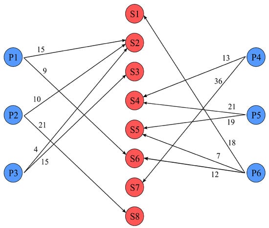
Figure 4.
Graphical interpretation of lowest cost solution.
The solution of transportation problem obtained by used methods and deviation from the lowest cost solution are summarized in Table 9. Solutions obtained by NW, MKW, and MK methods were not optimal, and therefore the potentials method was used.
Table 9.
Objective function and deviation from lowest cost solution.
4. Results
4.1. Optimization of the Basic Feasible Solution
Based on the input data set and the basic feasible solution obtained by the northwest corner method, the results table was first prepared so that the cells corresponding to supply and demand values remained empty. The transportation costs in the base cells were supplemented. It is assumed that the value of the potential is . The cost corresponding to this potential should be found and then the potential being the difference between the cost and potential should be calculated. In the task, we obtained the following values . The next cost in the column that corresponds to the should be found and the should be determined. The potential corresponding to the determined cost should be calculated as the difference between cost 1011 and potential . The procedure was repeated to determine the remaining potentials. The remaining cells should be filled in with the sums of potentials where and keeping in mind that n is the number of recipients and m is the number of suppliers [55]. The results of the applied conversions are shown in Table 10.
Table 10.
Summary of indirect costs and costs resulting from task content.
In the next step, the values of optimization indicators should be determined, understood as the difference between indirect costs and costs resulting from the numerical data. They are listed in Table 11.
Table 11.
Values of optimization indicators for solution obtained using northwest corner method.
There are positive numbers among the indicators, which means that the solution obtained is not optimal. The cycle design leads to an feasible solution at a lower cost. The first element of the positive cycle corresponds to the maximum optimization indicator. In a row containing an element of a positive cycle, the component that will have its equivalent in the column should be indicated. The procedure should be repeated until the cycle is closed. The lowest value from the components of the negative cycle must then be indicated and subtracted from all components of the negative cycle and added to all components of the positive cycle. The created cycle and the new feasible solution are shown in Table 12.
Table 12.
Cycle design and new feasible solution.
The cost of the current solution is €162,883.0, so it is slightly lower than the one obtained in the basic feasible solution, which means that the obtained solution is better. By repeating the above procedure 12 times, a new feasible solution was obtained. The feasible solution and the final values of the optimization indicators for the northwest corner method are presented in Table 13.
Table 13.
New solution and optimization indicators.
All values of the optimization indicators are negative, so the received solution of €102,152.0 is optimal. The final transportation costs and the result of the potential method leading to an optimal solution are presented in Table 14.
Table 14.
Comparison of methods and costs of solutions (€) obtained.
As can be seen from Table 14, the presented scheme of optimization of the obtained optimal solution was repeated:
- twelve times for the northwest corner method,
- seven times for the row minimum method,
- six times for the least cost in the matrix method,
- once for the VAM method.
Values of the transportation costs after subsequent steps of improvement are illustrated in Figure 5 and Figure 6.
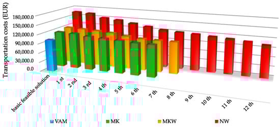
Figure 5.
Next improvements of solutions.
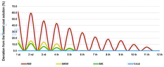
Figure 6.
Deviation from optimal solution.
4.2. Fuel Consumption and CO Emissions
The evolution of the transport system has a significant impact on the socioeconomic development of the modern world. The concept of sustainable transport takes into account not just economic and social criteria, but also environmental ones. Despite the significant role of the transport system in the development of the economy, transport has a negative impact on the quality of life and health of people, as well as on the environment due to its significant contribution to greenhouse gas emissions. International cooperation cannot be limited only to the expansion of the transport network (although this is an important aspect), but must also take environmental preservation into account. Sustainable transport development and environmental preservation are linked to the formation of a green transport system. Under the European Green Deal Communication [56], the European Union (EU) member states have committed to reducing greenhouse gas emissions by at least 55% by 2030, compared to 1990 levels. As part of the development of the market for low- and zero-emission vehicles, the European Commission has adopted the following targets for reducing CO emissions from newly manufactured passenger cars and delivery vehicles: a 55% reduction in CO emissions from passenger cars and a 50% reduction in CO emissions from delivery vehicles by 2030; zero CO emissions from new passenger cars by 2035. For new trucks, the target is to reduce CO emissions by an average of 15% from 2025 and 30% from 2030 when compared to 2019 levels. CO emissions from trucks, buses and coaches currently account for 6% of total EU CO emissions and 27% of total road transport CO emissions [57]. It is therefore necessary to adopt an environmentally friendly transport policy and to create tools to support decision-making processes, depending on the criteria adopted. Table 15 illustrates the total distance traveled expressed in (km), depending on the successive solutions obtained by the potential method.
Table 15.
Distance traveled (km) depending on solution obtained.
The calculations show that the basic feasible solution determined by the northwest corner method required the longest route of 11,226.0 (km). The optimal solution in terms of transport cost determined by the northwest corner method was not optimal in terms of total distance traveled. In the case of the least cost in the matrix method, the shortest distance required to complete the transport task equal to 6597.0 (km) was obtained as the result of the fifth iteration of the potential method. Of all the methods considered, the shortest route equal to 6559.0 (km) corresponded to the fourth iteration of the potentials method applied to the basic feasible solution determined by the row minimum method. A graphical interpretation of the results obtained is shown in the Figure 7.
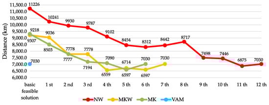
Figure 7.
Distance traveled (km) depending on different solutions obtained using potentials method.
The values of fuel consumption and CO emissions depending on the distance traveled are presented in Table 16. The Vehicle Energy Consumption Calculation Tool (VECTO version 3.3.9.2175) was used to calculate them [58].
Table 16.
Total fuel consumption and total CO emissions as a function of distance traveled.
Implementation of the transport plan in accordance with the basic solution determined by the northwest corner method is associated with the highest CO emissions of 4939.4 (kg). From an environmental point of view, the optimal solution offering the lowest CO emission of 2886.0 (kg) was obtained using the row minimum method as a result of applying the potentials method four times. The resulting solution leads to a reduction in total CO emissions by as much as 2053.5 (kg). The results of the performed calculations are shown in Figure 8.
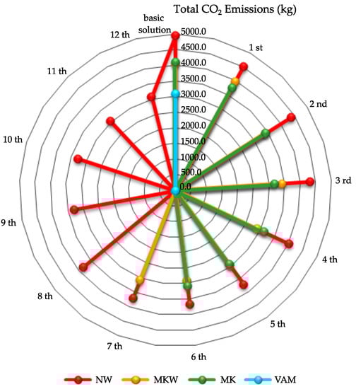
Figure 8.
CO emissions (kg) depending on solution obtained.
5. Discussion and Conclusions
The essential element of the logistic system is the subsystem of movement and transportation, whose main task is to ensure the timely movement of personnel and goods. The constant development of the automotive industry, the introduction of vehicles with increasing payloads and the ability to cross a variety of terrain, and the expansion of the road network indicate the growing importance of road transport. The dynamic change of the situation causes the distances of the supply routes to constantly change, which requires organizational effort. It is particularly important to be able to optimize the operations of road transport, especially when the time to make decisions is limited. There are many studies available in the literature concerning the optimization of the transportation problem depending on the established objective function, while taking into account the existing constraints.
The solutions used are aimed not only at determining the best method of solving the transportation problem, but also at developing an algorithm that leads to a reduction of calculation complexity by reducing the time needed for completing the calculations. The literature repeatedly addressed the possibilities of using the C++ programming language or the Matlab environment to increase the efficiency of the transportation algorithm, whereas division of source codes in GNU Octave was not yet research subject. More and more tools are now available for using programming techniques or performing complex numerical calculations, including a free GNU Octave environment. Determining the optimal solution of the transportation problem using the GNU Octave software was not yet considered in any publication. Therefore, the purpose of this article was to present an innovative approach to solving the transportation problem aimed at minimizing the transportation costs, fuel consumption, and CO emissions using programming in the GNU Octave.
Proposed solution using the GNU Octave has great practical and theoretical importance. The programming in GNU Octave saves a lot of time from complex and iterative calculations. The solutions used are aimed not only at determining the best method of solving the transportation problem, but also at decision support for individually defined criteria in other linear programming problems. The presented model was supported by a numerical example together with an interpretation of the results obtained. The paper focuses on determining the optimal method of product distribution within an assumed supply network using: the northwest corner, the least cost in the matrix, the row minimum and the Vogel Approximation Method (VAM) methods to calculate the minimal value of the objective function. A distribution network consisting of six suppliers and eight recipients of materials was considered. The transport was carried out with medium load trucks for which the cost ratio per unit of operation was €.
On the basis of the calculations carried out, it was found that determining the basic feasible solution for each of the presented methods required 14 iterations. When comparing the initial basic solutions of the problem in question, the values of the objective function varied according to the method used. The analysis shows that the highest cost of transport was obtained using the northwest corner method, which is the simplest to calculate but the least accurate. In turn, the least cost in the matrix method provided a lower value of the objective function than the commonly used row minimum method. The lowest transportation cost was obtained by means of the Vogel approximation. For each of the methods used, the necessary condition for the degeneration of the calculated feasible solution was met, which made it possible to apply the potentials method. Determining the optimal solution based on the northwest corner method required as much as twelve repetitions of the scheme for calculating the optimization indicators. The negative values of the optimization indicators were obtained in the case of the row minimum method after seven repetitions of the scheme. The application of the least cost in the matrix method required six repetitions of the potential method.
The evolution of the transport system has a significant impact on the socioeconomic development of the world. However, it should be emphasized that despite economic growth, transport has a negative impact on the environment through its significant contribution to greenhouse gas emissions. Therefore, it is necessary to implement a proecological transport policy and to develop tools to support rational decision-making depending on the criterion adopted. We propose one such tool, provided in the form of attached source codes, only requiring the user to enter numerical data. Taking into account the ecological aspect, it was observed that the implementation of the transport task in accordance with the basic feasible solution obtained from the northwest corner method results in a total of (kg) of CO being emitted into the atmosphere, while the application of the fourth iteration of the potentials method in relation to the row minimum method reduces CO emissions to (kg), which amounts to %. The optimal solution obtained in this way reduces the total CO emissions by as much as (kg).
The implementation of the proposed solution shortens the calculation algorithm and allows the user to determine the optimal distribution plan for material resources for individually determined criteria. The advantage of the software used is that the GNU Octave command window displays the individual steps leading to the basic feasible solution for each of the methods presented. In addition, an attempt by the user to enter negative numbers generates a message that the entered values must be changed. Moreover, the source code for each of the methods checks whether the distribution network under consideration is a so-called balanced transportation problem. The disadvantage of the software used is that if the user inputs the data incorrectly, it is necessary to reinput all data again.
The use of IT tools allows effective management of the vehicle fleet and provides the possibility of organizing the workload of drivers to perform initial calculations of the costs at the planning stage of the transport operations. The increasing computing power of computers provides the ability to solve increasingly complex decision-making problems. Therefore, the right direction of further research will be to extend the function of the program with an algorithm based on the potentials method and to use the Gnuplot graphic tool to visualize the results in the form of a graph of the optimal distribution network.
Author Contributions
Conceptualization, J.M. and J.S.-R.; methodology, J.Z. and J.S.-R.; software, J.S.-R.; validation, J.S.-R.; formal analysis, J.M. and J.S.-R.; investigation, J.S.-R.; resources, J.S.-R. and J.Z.; data curation, J.S.-R. and M.O.; writing—original draft preparation, J.S.-R.; writing—review and editing, J.S.-R.; visualization, J.S.-R.; supervision, J.S.-R. All authors have read and agreed to the published version of the manuscript.
Funding
This research received no external funding.
Institutional Review Board Statement
Not applicable.
Informed Consent Statement
Not applicable.
Data Availability Statement
Not applicable.
Acknowledgments
This work was supported by Military University of Technology (project No.878/ WAT/2021). This support is gratefully acknowledged.
Conflicts of Interest
The authors declare no conflict of interest.
Appendix A


Appendix B


Appendix C


Appendix D


References
- Angelelli, E.; Morandi, V.; Savelsbergh, M.; Speranza, M.G. System optimal routing of traffic flows with user constraints using linear programming. Eur. J. Oper. Res. 2021, 293, 863–879. [Google Scholar] [CrossRef]
- Barnhart, C.; Krishnan, N.; Kim, D.; Ware, K. Network design for express shipment delivery. Comput. Optim. Appl. 2002, 21, 239–262. [Google Scholar] [CrossRef]
- Serrano-Hernandez, A.; Faulin, J.; Hirsch, P.; Fikar, C. Agent-based simulation for horizontal cooperation in logistics and transportation: From the individual to the grand coalition. Simul. Model. Pract. Theory 2018, 85, 47–59. [Google Scholar] [CrossRef]
- Mancini, S.; Gansterer, M. Vehicle routing with private and shared delivery locations. Comput. Oper. Res. 2021, 133, 105361. [Google Scholar] [CrossRef]
- Tamannaei, M.; Rasti-Barzoki, M. Mathematical programming and solution approaches for minimizing tardiness and transportation costs in the supply chain scheduling problem. Comput. Ind. Eng. 2019, 127, 643–656. [Google Scholar] [CrossRef]
- Salehi, M.; Jalalian, M.; Vali Siar, M. Green transportation scheduling with speed control: Trade-off between total transportation cost and carbon emission. Comput. Ind. Eng. 2017, 113, 392–404. [Google Scholar] [CrossRef]
- Żurek, J.; Małachowski, J.; Ziółkowski, J.; Szkutnik-Rogoż, J. Reliability analysis of technical means of transport. App. Sci. 2020, 10, 3016. [Google Scholar] [CrossRef]
- Sagratella, S.; Schmidt, M.; Sudermann-Merx, N. The noncooperative fixed charge transportation problem. Eur. J. Oper. Res. 2020, 284, 373–382. [Google Scholar] [CrossRef]
- Tang, C.H. Optimization for transportation outsourcing problems. Comput. Ind. Eng. 2020, 139, 106213. [Google Scholar] [CrossRef]
- Fricker, J.; Whitford, R. Fundamentals of transportation engineering. In A Multimodal Systems Approach; Pearson Education, Inc.: Upper Saddle River, NY, USA, 2004. [Google Scholar]
- Ozkok, B.A. An iterative algorithm to solve a linear fractional programming problem. Comput. Ind. Eng. 2020, 140, 106234. [Google Scholar] [CrossRef]
- Venkatachalapathy, M.; Pandiarajan, R.; Ganeshkumar, S. A special type of solving transportation problems using generalized quadratic fuzzy number. Int. J. Sci. Technol. Res. 2020, 9, 6344–6348. [Google Scholar]
- Kuiteing, A.K.; Marcotte, P.; Savard, G. Pricing and revenue maximization over a multicommodity transportation network: The nonlinear demand case. Comput. Optim. Appl. 2018, 71, 641–671. [Google Scholar] [CrossRef]
- Cosma, O.; Pop, P.C.; Dănciulescu, D. A novel matheuristic approach for a two-stage transportation problem with fixed costs associated to the routes. Comput. Oper. Res. 2020, 118, 104906. [Google Scholar] [CrossRef]
- Bamigboye, O.; Olufunke, O.; Agarana, M.; Olabode, O. Optimizing the movement of people and goods in a local community using transportation model. In Proceedings of the 2nd International Conference on Engineering for Sustainable World, Ota, Nigeria, 9–13 July 2018; Volume 413, p. 012020. [Google Scholar] [CrossRef]
- Selech, J.; Andrzejczak, K. An aggregate criterion for selecting a distribution for times to failure of components of rail vehicles. Maint. Rel. 2020, 22, 102–111. [Google Scholar] [CrossRef]
- Levinson, H. The reliability of transit service: An historical perspective. J. Urban Technol. 2005, 12, 99–118. [Google Scholar] [CrossRef]
- Adlakha, V.; Kowalski, K. Alternate solutions analysis for transportation problems. J. Bus. Econ. Res. 2011, 7, 41–49. [Google Scholar] [CrossRef]
- Andrzejczak, K.; Młyńczak, M.; Selech, J. Poisson-distributed failures in the predicting of the cost of corrective maintenance. Maint. Rel. 2018, 20, 602–609. [Google Scholar] [CrossRef]
- Żurek, J.; Ziółkowski, J.; Szkutnik-Rogoż, J. Stochastic dominance application for optimal transport company selection. In Proceedings of the 15th Conference on Computational Technologies in Engineering, TKI 2018, Jora Wielka, Poland, 16–19 October 2018; p. 020074. [Google Scholar] [CrossRef]
- Ziółkowski, J.; Oszczypała, M.; Małachowski, J.; Szkutnik-Rogoż, J. Use of artificial neural networks to predict fuel consumption on the basis of technical parameters of vehicles. Energies 2021, 14, 2639. [Google Scholar] [CrossRef]
- Azucena, J.; Alkhaleel, B.; Liao, H.; Nachtmann, H. Hybrid simulation to support interdependence modeling of a multimodal transportation network. Simul. Model. Pract. Theory 2021, 107, 102237. [Google Scholar] [CrossRef]
- Hitchcock, F. The distribution of a product from several sources to numerous localities. J. Math. Phys. 1941, 20, 224–230. [Google Scholar] [CrossRef]
- Dantzig, G. Application of the Simplex Method to a Transportation Problem, Activity Analysis of Production and Allocation; Koopmans, T.C., Ed.; John Wiley & Sons: New York, NY, USA, 1951. [Google Scholar]
- Charnes, A.; Cooper, W.; Henderson, A. An Introduction to Linear Programming; John Wiley & Sons: New York, NY, USA, 1953. [Google Scholar]
- Mhlanga, A.; Nduna, I.S.; Matarise, D.F.; Machisvo, A. Innovative application of Dantzig’s North–West Corner Rule to solve a transportation problem. Int. J. Educ. Res. 2014, 2, 1–12. [Google Scholar]
- Loch, G.V.; da Silva, A.C.L. A computational study on the number of iterations to solve the transportation problem. Appl. Math. Sci. 2014, 8, 4579–4583. [Google Scholar] [CrossRef][Green Version]
- Can, T.; Koçak, H. Tuncay Can’s Approximation Method to obtain initial basic feasible solution to transport problem. Appl. Comput. Math. 2016, 5, 78–82. [Google Scholar] [CrossRef][Green Version]
- Karagul, K.; Sahin, Y. A novel approximation method to obtain initial basic feasible solution of transportation problem. J. King Saud Univ. Eng. Sci. 2020, 32, 211–218. [Google Scholar] [CrossRef]
- De França Aguiar, G.; De Cássia Xavier Cassins Aguiar, B.; Wilhelm, V. New methodology to find initial solution for transportation problems: A case study with fuzzy parameters. Appl. Math. Sci. 2015, 9, 915–927. [Google Scholar] [CrossRef]
- Korukoǧlu, S.; Balli, S. An improved Vogel’s approximation method for the transportation problem. Math. Comput. Appl. 2011, 16, 370–381. [Google Scholar] [CrossRef]
- Das, U.K.; Babu, A.; Khan, A.R.; Helal, A.; Uddin, D.S. Logical development of Vogel’s approximation method (LD-VAM): An approach to find basic feasible solution of transportation problem. Int. J. Sci. Technol. Res. 2014, 3, 42–48. [Google Scholar]
- Ahmed, M.M.; Khan, A.R.; Uddin, M.S.; Ahmed, F. A new approach to solve transportation problems. Open J. Optim. 2016, 5, 22–30. [Google Scholar] [CrossRef]
- Kirca, O.; Şatir, A. A heuristic for obtaining an initial solution for the transportation problem. J. Oper. Res. Soc. 1990, 41, 865–871. [Google Scholar] [CrossRef]
- Mathirajan, M.; Meenakshi, B. Experimental analysis of some variants of Vogel’s approximation method. Asia-Pac. J. Oper. Res. 2004, 21, 447–462. [Google Scholar] [CrossRef]
- Juman, Z.; Hoque, M. An efficient heuristic to obtain a better initial feasible solution to the transportation problem. Appl. Soft Comput. 2015, 34, 813–826. [Google Scholar] [CrossRef]
- Imam, T.; Elsharawy, G.; Gomah, M.; Samy, I. Solving transportation problem using object-oriented model. Int. J. Comput. Sci. Netw. Secur. 2009, 9, 353–361. [Google Scholar]
- Pallavi, P.L.; Lakshmi, R.A. A Mat Lab oriented approach to solve the transportation problem. Int. J. Adv. Res. Found. 2015, 50, 6000. [Google Scholar]
- Appati, J.K.; Gogovi, G.K.; Fosu, G.O. MATLAB implementation of Vogel’s approximation and the modified distribution methods. Int. J. Adv. Comput. Technol. 2015, 4, 1449–1453. [Google Scholar]
- Ghadle Kirtiwant, P.; Muley Yogesh, M. New approach to solve assignment problem using MATLAB. Int. J. Latest Technol. Eng. Manag. Appl. Sci. 2015, 4, 36–39. [Google Scholar]
- Sengamalaselvi, D.J. Solving transportation problem by using MATLAB. Int. J. Eng. Sci. Res. Technol. 2017, 6, 374–381. [Google Scholar] [CrossRef]
- Chung, K.J. The integrated inventory model with the transportation cost and two-level trade credit in supply chain management. Comput. Math. Appl. 2012, 64, 2011–2033. [Google Scholar] [CrossRef]
- Juman, Z.; Hoque, M. A heuristic solution technique to attain the minimal total cost bounds of transporting a homogeneous product with varying demands and supplies. Eur. J. Oper. Res. 2014, 239, 146–156. [Google Scholar] [CrossRef]
- Mandal, J.; Goswami, A.; Wang, J.; Tiwari, M. Optimization of vehicle speed for batches to minimize supply chain cost under uncertain demand. Inf. Sci. 2020, 515, 26–43. [Google Scholar] [CrossRef]
- Pielecha, J.; Skobiej, K.; Kurtyka, K. Exhaust emissions and energy consumption analysis of conventional, hybrid, and electric vehicles in real driving cycles. Energies 2020, 13, 6423. [Google Scholar] [CrossRef]
- Berling, P.; Martínez-De-Albéniz, V. Dynamic speed optimization in supply chains with stochastic demand. Transp. Sci. 2016, 50, 1114–1127. [Google Scholar] [CrossRef]
- Galińska, B. Multiple criteria evaluation of global transportation system—Analysis of case study. In Proceedings of the 14th Scientific and Technical Conference on Transport Systems Theory and Practice, TSTP 2017, Katowice, Poland, 18–20 September 2017; pp. 155–171. [Google Scholar]
- Entrialgo, J.; García, M.; Díaz, J.; García, J.; García, D.F. Modelling and simulation for cost optimization and performance analysis of transactional applications in hybrid clouds. Simulat. Model. Pract. Theory 2021, 109, 102311. [Google Scholar] [CrossRef]
- Das, A.; Deepmala, J.R. Some aspects on solving transportation problem. Yugosl. J. Oper. Res. 2020, 30, 45–57. [Google Scholar] [CrossRef]
- Kramer, R.; Maculan, N.; Subramanian, A.; Vidal, T. A speed and departure time optimization algorithm for the pollution-routing problem. Eur. J. Oper. Res. 2015, 247, 782–787. [Google Scholar] [CrossRef]
- Wang, M.H.; Kuo, Y.E. A perturbation method for solving linear semi-infinite programming problems. Comput. Math. Appl. 1999, 37, 181–198. [Google Scholar] [CrossRef][Green Version]
- Cyplik, P.; Głowacka-Fertsch, D.; Fertsch, M. Logistics of Distribution Companies; ILiM: Poznań, Poland, 2008. [Google Scholar]
- Cieśla, M.; Sobota, A.; Jacyna, M. Multi-Criteria decision making process in metropolitan transport means selection based on the sharing mobility idea. Sustainability 2020, 12, 7231. [Google Scholar] [CrossRef]
- Bozarth, C.; Handfield, R. Introduction to Operations and Supply Chain Management, 5th ed.; Pearson Education: Upper Saddle River, NJ, USA, 2019. [Google Scholar]
- Gehlot, H.; Honnappa, H.; Ukkusuri, S. An optimal control approach to day-to-day congestion pricing for stochastic transportation networks. Comput. Oper. Res. 2020, 119, 104929. [Google Scholar] [CrossRef]
- Available online: https://eur-lex.europa.eu/legal-content/EN/TXT/PDF/?uri=CELEX:52021PC0556&from=EN (accessed on 8 September 2021).
- Available online: https://www.consilium.europa.eu/pl/press/press-releases/2019/06/13/cutting-emissions-council-adopts-co2-standards-for-trucks/ (accessed on 8 September 2021).
- Available online: https://ec.europa.eu/clima/policies/transport/vehicles/vecto_en (accessed on 12 August 2021).


Publisher’s Note: MDPI stays neutral with regard to jurisdictional claims in published maps and institutional affiliations. |
© 2021 by the authors. Licensee MDPI, Basel, Switzerland. This article is an open access article distributed under the terms and conditions of the Creative Commons Attribution (CC BY) license (https://creativecommons.org/licenses/by/4.0/).