Abstract
Often, second law-based studies present merely entropy calculations without demonstrating how and whether such calculations may be beneficial. Entropy generation is commonly viewed as lost work or sometimes a source of thermodynamic losses. Recent literature reveals that minimizing the irreversibility of a heat engine may correspond to maximizing thermal efficiency subject to certain design constraints. The objective of this article is to show how entropy calculations need to be interpreted in thermal processes, specifically, where heat-to-work conversion is not a primary goal. We will study four exemplary energy conversion processes: (1) a biomass torrefaction process where torrefied solid fuel is produced by first drying and then torrefying raw feedstock, (2) a cryogenic air separation system that splits ambient air into oxygen and nitrogen while consuming electrical energy, (3) a cogeneration process whose desirable outcome is to produce both electrical and thermal energy, and (4) a thermochemical hydrogen production system. These systems are thermodynamically analyzed by applying the first and second laws. In each case, the relation between the total entropy production and the performance indicator is examined, and the conditions at which minimization of irreversibility leads to improved performance are identified. The discussion and analyses presented here are expected to provide clear guidelines on the correct application of entropy-based analyses and accurate interpretation of entropy calculations.
1. Introduction
The two main laws of thermodynamics, originally founded on heat engines in the 19th century, have been applied frequently to study energy systems. The first law, an expression of the principle of energy conservation, allows to measure the conversion of one form of energy to another, i.e., heat and work, in a system. The second law measures the degree of irreversibility of the system in terms of entropy production. The concept of entropy generation and its relation to work production in an irreversible engine was first introduced by Clausius; it later provided a basis for introducing subsequent concepts such as availability. However, is irreversibility unconditionally a performance indicator in a thermodynamic process? From a design perspective, do the two laws applied to an energy system yield identical or different outcomes? Is minimization of irreversibility desired? Entropy generation is sometimes viewed as a measure of lost work. This notion is correct in heat-work conversion systems, e.g., a power cycle, subject to certain design constraints [1,2].
The equivalence of minimum irreversibility and maximum thermal efficiency, and/or maximum work in heat-work conversion processes have been investigated by several authors [3,4,5,6,7,8,9,10,11,12,13,14]. The key conclusion from these past studies is that the regime of minimum entropy production is identical to that of maximum efficiency and maximum power under specific design conditions, for instance, if the heat input is treated as a fixed quantity. Alternatively, if the power output is fixed, the design at minimum entropy production is identical to that of maximum thermal efficiency. In 1996, Bejan [6,7] highlighted a key but usually overlooked source of entropy generation associated with the operation of heat engines: the irreversible cooling process of exhaust stream that should be included in the calculation of the total entropy production. In many practical applications, e.g., engines, ships, combined cycle power plants, gas turbine cycles, flue gases are discharged to the atmosphere. He presented models of endoreversible heat engines that would produce maximum work at minimum entropy generation at which the efficiency is obtained by
where TH and TL denote the temperatures of the hot and cold thermal reservoirs, respectively. Equation (1) is known as the maximum power efficiency in endoreversible engines, often attributed to Curzon and Ahlborn [15,16,17]. However, its derivation can be found in Cotterill’s book [18], published in the late 19th century.
In general, without the specific design constraints mentioned previously, the minimum irreversibility, maximum efficiency, and maximum power are different design criteria. To rectify this issue in combustion-driven power systems, Haseli [19] introduced the concept of specific entropy generation (SEG), defined as the total entropy production per unit consumption of fuel. It is shown that the thermal efficiency of a gas turbine cycle or a combined cycle power plant [20] correlates unconditionally with SEG. Indeed, it can be shown that maximum thermal efficiency is always equivalent to minimum SEG in power generating systems driven by fuel oxidation [21].
Often, entropy-based studies present merely entropy calculations without demonstrating how and if such calculations may be used to improve system efficiency. The question that forms the basis of the present article is: what do irreversibility and entropy production represent in energy systems where the primary (or only) objective is not to produce (or consume) work through conversion of thermal energy, and under what conditions a designer could benefit from entropy analyses? Examples include biomass torrefaction plant, cryogenic air separation unit, cogeneration process, hydrogen production plant, fluidized bed, solid fuel gasification, steam condenser, biofuel production through pyrolysis, and oxyfuel combustion. To answer the above questions, we will thermodynamically analyze the first four systems listed above. In each case, the possibility of any relation between the performance indicator and the irreversibility of the system will be examined. The four chosen energy systems are simply arbitrary since the main goal is to show that irreversibility is not necessarily an indication of imperfectness in an energy conversion system. The conditions at which minimum entropy production may lead to an improved performance will be discussed for each of the four systems.
2. Biomass Torrefaction Process
The primary objective in a torrefaction process is to produce high-quality fuel material (i.e., torrefied biomass) through thermochemically treating the raw biomass [22,23]. The process requires thermal energy, which is supplied by burning a utility fuel and torrefaction gases [24]. The main components and a simplified layout of a torrefaction process are depicted in Figure 1. In practice, the torrefied material is ground and then pelletized (not shown in Figure 1) through the consumption of power.
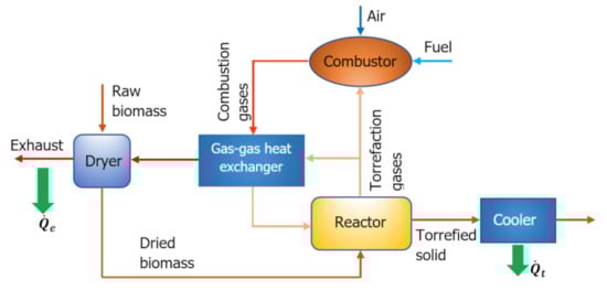
Figure 1.
The layout of a biomass torrefaction plant.
Raw biomass with a moisture content of MC (% dry basis) is first dried in a dryer. In the torrefaction reactor, the dried biomass undergoes mild pyrolysis at a temperature in the range of 200–300 °C. A portion of the volatiles leaving the torrefaction process is recycled back to the reactor and is used as the inert gas. The rest of the volatiles are burned together with an auxiliary fuel (e.g., methane) in a combustor. The torrefied solid leaving the reactor is cooled in a heat exchanger. The heat requirement of the drying and torrefaction is provided by the combustion products.
The first law for the system of Figure 1 may be written as follows.
where is the total enthalpy at the ambient conditions, superscripts a, r, f, t, p, w denote, air, raw biomass, auxiliary fuel, torrefied biomass, combustion products, the water content in raw biomass, respectively, and is the total amount of heat discharged from the process to the atmosphere through the reaction products, (combustion products plus the moisture content of biomass) and the torrefied solid cooler, ; see Figure 1.
On the other hand, the following relation is obtained from an entropy analysis of the system.
where is the rate of total entropy generation associated with the torrefaction process, T0 the surroundings temperature, and S the entropy.
Indeed, one could obtain Equation (3) by adding the entropy generation rates associated with the operation of the individual components, i.e., dryer, heat exchanger, combustor, torrefaction reactor, and cooler, plus that due to the cooling of the exhaust stream in accordance with Bejan’s argument [6,25] as discussed in the preceding section.
A combination of Equations (2) and (3) yields
Notice that Equation (4) includes entropy generation (exergy destruction, ) term, but unlike in a combustion engine, no power generation is associated with the torrefaction process. So, interpretation of entropy generation as a measure of lost work would be irrelevant here because the purpose of a torrefaction plant is to produce torrefied biomass (a desired outcome) through thermochemically treating raw biomass. It would therefore be necessary to clarify what exergy destruction represents in a torrefaction process and whether its minimization could lead to improved performance.
A frequently used performance indicator of a biomass torrefaction process is energy yield, defined as [26]
where denotes the mass flowrate, and HHV is the higher heating value.
The performance of the process may also be measured from a pure thermal energy perspective.
where ηth is the thermal efficiency and LHV is the lower heating value. The overall efficiency of the process (ηov) should account for the quantity of electrical energy consumed in Equation (6).
Before applying an entropy or exergy analysis, one must determine, a priori, if and under what conditions minimization of entropy generation () or exergy destruction () could lead to improved performance. Unless a performance indicator (YE, ηth, or ηov) correlates inversely with , a second-law analysis of the torrefaction process would be of no practical significance.
Let us examine whether minimizing correlates with maximization of . Per unit flowrate of dry biomass, the required mass flowrates of the air and methane are determined as follows [24].
where is the volatiles yield, MW denotes the molecular weight, and are stoichiometric coefficients of the air and methane, respectively.
The mass flow rate of the combustion products may then be obtained from the mass conservation of the combustor. Hence,
Using Equations (7)–(9), one may rewrite Equation (4) per unit flow rate of the dry biomass as
where , and denote specific enthalpy and specific entropy, respectively.
Both bracketed terms on the right side of Equation (10) are fixed. So, the specific entropy generation (SEG) is proportional to the volatiles yield. Whether decreases or increases with an increase in depends on the coefficient of (the first bracketed term) in Equation (10).
Likewise, one may find a relation for the thermal efficiency of the process defined in Equation (6) as a function of the volatiles yield. Denoting the solid mass yield by where , substituting Equation (8) into Equation (6) and rewriting per unit mass flow rate of the dry biomass, we get
From a previous study [27], it can be shown that
where and are numerical constant.
Substituting Equation (12) into Equation (11) and differentiating with respect to , one obtains
This result reveals that the volatiles yield has an inverse effect on the thermal efficiency. The main conclusion from the above analysis is that minimization of SEG corresponds to maximization of the thermal efficiency for the torrefaction system of Figure 1 if the coefficient of in Equation (10) is positive. Determination of the coefficient of the volatiles yield is not a straightforward task as it includes several parameters (e.g., ). For this, one would need a comprehensive model [24,28]. Such a task is, however, beyond the scope of the present article.
3. Cryogenic Air Separation Process
In a cryogenic air separation unit (ASU), atmospheric air is split into a stream of oxygen and a nitrogen stream. The process requires electrical energy input that is primarily used for compression of the air. Figure 2 shows the layout of a cryogenic ASU, very much like that designed by Allam [29], which consists of two air compressors, two air turbines, the main heat exchanger, a double-column distillation, an air cooler, an oxygen pump, and an adsorption unit. Application of the ASU depicted in Figure 2 in a supercritical CO2 power cycle has been reported in reference [30].
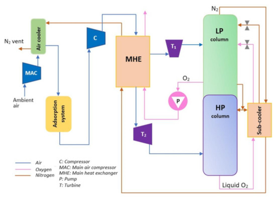
Figure 2.
Schematic of a cryogenic air separation unit.
Ambient air is pressurized to 5 bar within the main air compressor (MAC). The cooler is used to decrease the temperature of the air stream pressurized in MAC. Impurities of the cool air are removed in the adsorption system. The pressure of the purified air is further increased in the booster compressor. The pressurized air leaving the booster is first cooled (not shown in Figure 2) and then sent to the main heat exchanger (MHE), where the cold oxygen and nitrogen streams produced in the distillation unit are warmed by the air stream. As shown in Figure 2, the air flow is split within MHE into two streams. One stream is expanded in the first turbine down to 1.2 bar, whereas the second stream is expanded in the second turbine to 5 bar. The exhaust streams of the turbines are fed to the columns of the distillation unit.
The first law applied to the system of Figure 2 may be expressed as
where denotes the net power requirement of the ASU.
Also, accounts for the total rate of heat rejected from the ASU to the surroundings. Heat is discharged to the outside of the boundary of ASU due to cooling the air streams after MAC and the booster. For simplicity of the analysis, we assume that the air stream at the exit of both ASU compressors is cooled by rejecting sensible heat to the surroundings that is at T0.
The entropy balance equation of the system of Figure 2 is
Notice that Equations (14) and (16) are written assuming that both oxygen and nitrogen streams leaving the ASU are at T0. A combination of Equations (14) and (16) to eliminate the heat transfer term yields
where denotes a modified Gibbs function [31].
It can be inferred from Equation (17) that minimization of entropy production rate may lead to a minimum ASU power consumption if the algebraic summation of the three Gm terms is constant. Assuming the composition of the ambient air as 0.21O2/0.79N2 and denoting the molar flow rate of the air by , we have
Likewise, for the oxygen and nitrogen leaving the ASU, one may write
A further simplifying assumption is that all three gases behave like ideal gases. Thus, the specific enthalpy h is a function of temperature only. Because the inlet and outlet streams are at T0, the difference between Gm of the air and Gm of the “oxygen + nitrogen” will depend on the entropies of the oxygen and nitrogen. Note that the enthalpy terms will cancel out. Hence,
where
where is the pressure of component i (oxygen, nitrogen) at the exit of ASU, denotes the partial pressure of component i in air, and is the universal gas constant.
Substituting Equations (22) and (23) into Equation (21) gives
The partial pressures of oxygen and nitrogen in the air are fixed. In most cryogenic air separation systems, the exit pressure of oxygen and nitrogen streams is around atmospheric pressure so and may be treated as fixed quantities. The right side of Equation (24) will be fixed if the air flow rate is a given quantity. In this case, minimization of will guarantee that will also be a minimum; see Equation (17). It can be concluded that the equivalence is subject to the pressure of the oxygen and nitrogen streams leaving the ASU at T0, as well as the air flow rate being constant.
Nevertheless, if either temperature or pressure of either of the exiting streams occurs to be a variable, the algebraic sum of the three Gm terms in Equations (21) and (24) will no longer be a constant. In this case, minimizing the entropy generation rate associated with the operation of the ASU will not necessarily be equivalent to the minimization of its power requirement. On the other hand, one could perform the above analysis per unit flow rate of the air (or either of the exit streams) to express Equation (17) in terms of a specific entropy generation as follows.
where denotes the total entropy generation rate per unit flow rate of the air.
If the pressure of both oxygen and nitrogen streams exiting the ASU at T0 are fixed, the operation of the ASU at minimum will be equivalent to that at minimum specific power consumption, i.e., .
4. Cogeneration Process
The third energy system to be examined is a cogeneration process in that the hot exhaust of a power cycle is used to produce high-pressure saturated vapor [32]. As shown in Figure 3, air, fuel, and water are supplied at the ambient temperature and pressure. The low-temperature combustion products leaving the steam generator are discharged to the atmosphere. Applying the first law to the cogeneration process in Figure 3, we have
where is the total heat rate transferred to the water in the steam generator.
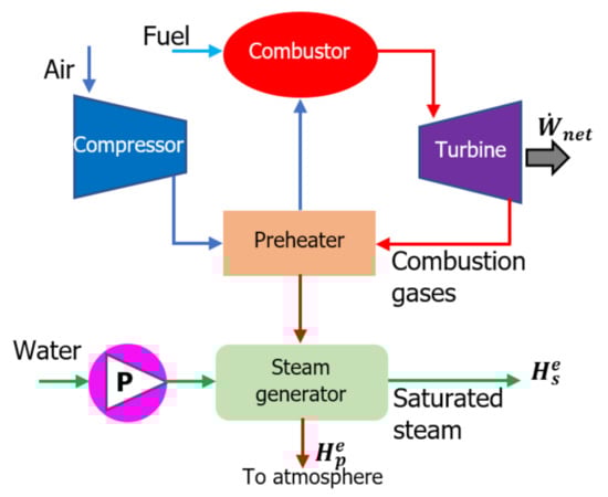
Figure 3.
Schematic of a cogeneration process.
The desired outcome in the cogeneration process is to generate not only power but also thermal energy [33,34]. The objective is then to maximize per the thermal energy liberated through the combustion of fuel. To burn each mole of the fuel represented by the chemical formula CxHyOz, 4.76Λ moles of air is required, whereby moles of combustion products are formed. Here, Λ is a stoichiometric coefficient that accounts for the quantity of air required to (i) ensure complete combustion and (ii) maintain combustion temperature at the desired level, . Indeed, Λ is inversely related to .
Dividing Equation (26) by the molar flow rate of the fuel yields
where denotes the molar flowrate of water per unit molar flow rate of the fuel, and is the net increase in the specific enthalpy of water.
In practice, the exhaust temperature of the combustion products, , should not fall below a certain limit to prevent water condensation and corrosion issues. For this, the enthalpy of the combustion gases at the exit of the system may reasonably be taken as a fixed parameter. Because the enthalpy of the incoming air and fuel are also fixed, one may conclude from Equation (28) that is a constant quantity; it is equivalent to a fixed cogeneration efficiency. This conclusion, of course, is valid for a preset combustion (adiabatic flame) temperature.
Applying an entropy balance to the cogeneration process depicted in Figure 3, expressed per unit molar flow rate of the fuel, we obtain
where is the net increase in the specific entropy of water.
The first three terms on the right side of Equation (27) are constant. Thus, minimization of SEG would be identical to minimization of the net increase in the water entropy, but it would not have an impact on the cogeneration efficiency, which, as discussed above, is a fixed quantity.
Let us now consider a more general scenario in that Λ (thus combustion temperature) is a variable. Equation (28) may be rewritten as
where and the enthalpy difference are both fixed. Thus, it can readily be inferred that maximizing the cogeneration efficiency requires the minimization of . On the other hand, in accordance with Equation (29), minimization of SEG would be identical to minimizing . Therefore, we conclude that minimization of SEG does not correspond to improving the cogeneration efficiency.
It is worth mentioning, yet an alternative scenario, in that the supplied flow rate and temperature of water are design constraints. In this case, optimization of the thermal efficiency and cogeneration efficiency will be equivalent. According to Equations (29) and (30), minimization of would lead to a maximum but a minimum SEG. In other words, the equivalence is subject to both the supply temperature and flow rate of the water being constant.
5. Hydrogen Production Plant
The next system is a thermochemical hydrogen production process (Figure 4). For each mole of water supplied at ambient conditions, one mole of hydrogen and a half mole of oxygen is produced through a series of reactions. Known as the copper-chlorine (Cu-Cl) cycle, the process requires thermal and electrical energy to split water into hydrogen and oxygen [35,36,37]. Superheated steam reacts with cupric chloride (CuCl2) solid particles in a fluidized bed (step 4 in Figure 4) to yield hydrochloric (HCl) gas and copper oxychloride (Cu2OCl2) solid. The former product reacts with copper particles (step 1) in another reactor producing hydrogen and cuprous chloride (CuCl) solid, whereas the latter is first heated up to ~500 °C and then it decomposes into oxygen and cuprous chloride (step 5). The CuCl streams leaving the hydrogen and oxygen production reactors are cooled to around ambient temperature.
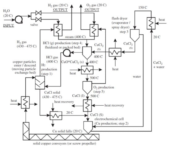
Figure 4.
Schematic of the copper-chlorine cycle for hydrogen production [36].
Next, the CuCl solid particles are mixed with a water stream, then undergo an electrolysis process (step 2), leading to the production of copper particles and aqueous cupric chloride. The copper particles are sent to the hydrogen production reactor (step 5). The moisture content of the aqueous cupric chloride is then removed in a dryer (step 3). The cupric chloride solids leaving the dryer at a moderate temperature are heated to ~400 °C and fed to the fluidized bed to react with the superheated steam (step 4). On the other hand, the water captured in the dryer is recycled back and mixed with CuCl particles before the electrolysis process (step 2). Note that all chemical compounds participating in the reactions, except supplied water, hydrogen, and oxygen formed in the process, circulate in a closed loop.
Thermodynamically, the Cu-Cl cycle interacts with its surroundings by admitting thermal energy through a heat transfer fluid supplied at , electrical work, and heat losses to the atmosphere that is at . As shown in Figure 4, there are opportunities for heat recovery whereby boosting the energy efficiency of the process. Nevertheless, recovering low-grade heat (e.g., from dryer) would practically be of no use [38], which is discharged to the atmosphere (part of the heat losses). A combined first and second laws expression applied to the Cu-Cl cycle of Figure 4 written per unit mole of hydrogen is
where is defined previously, see Equation (10), denotes the number of moles of the heat transfer fluid per unit mole of hydrogen, the superscript “e” is the state at the exit of the Cu-Cl cycle, and is the electrical energy required per mole of hydrogen produced in the process.
The state of the supplied water, hydrogen, and oxygen leaving the cycle is fixed. The first bracketed term on the right side of Equation (31) is, therefore, a fixed quantity. Further, the specific electrical energy required in the process is constant, according to previous studies [38,39]. We are then led to conclude that minimizing specific entropy generation would necessitate minimization of .
On the other hand, the overall efficiency of the copper-chlorine cycle is defined as
where denotes the heat-equivalent of the electrical energy and is a power production efficiency.
To maximize the overall efficiency, one would need to minimize in accordance with Equation (32). If minimization of occurs to be equivalent to minimization of , it may then be concluded that . Below, we examine three possible scenarios. Note that should be greater than the maximum temperature in the Cu-Cl cycle (~500 °C).
Suppose that in addition to the inlet temperature of the heat transfer fluid, , its number of moles per unit mole of hydrogen, , is also fixed. In this case, whereas . The pressure of the heat transfer fluid at the exit of the cycle is dependent on the pressure drop on the flow path; it may reasonably be taken as a design constraint. Thus, the thermodynamic properties and are solely a function of the exit temperature . The specific enthalpy is proportional to the temperature, so a higher would yield a higher . Differentiating and using the fundamental relation , we have
Since the coefficient of in Equation (33) is a positive quantity. So, an increase in will lead to an increase in . We may now conclude that the minimization of SEG will lead to the maximum overall efficiency of the Cu-Cl cycle.
An alternative scenario is that both inlet and outlet temperatures of the heat transfer fluid are fixed and is a design variable. It is obvious from Equation (31) that decreasing would lead to a lower SEG, whereas in accordance with Equation (32), it would increase the cycle efficiency. In other words, if the only design variable is , the operation at minimum SEG and maximum Cu-Cl cycle efficiency will be identical.
Consider now a third case in that the heat transfer fluid circulates in a closed loop, which, upon leaving the Cu-Cl cycle at is retuned to a thermal reservoir where it is heated up to . Denoting the temperature of the thermal reservoir by , the heat transfer coefficient and surface area by U and A, respectively, we have
Equation (34) provides a relationship between and . To maximize the overall efficiency, Equation (32), one then needs to minimize Equation (34). The right side of Equation (34) is a descending function of . That is, to maximize the efficiency of the copper-chlorine cycle, the temperature of the heat transfer fluid should be as high as possible at the exit of the cycle. Using Equation (34), we also find the following expression.
where is the (average) specific heat of the heat transfer fluid.
The right side of Equation (35) is, too, a decreasing function of . Thus, to minimize SEG, the exit temperature of the heat transfer fluid should be at its highest possible value. From this discussion and analysis, we conclude once again that there exists an inverse relation between SEG and cycle efficiency.
6. Conclusions
Four different energy systems have been examined through the first and second laws of thermodynamics: a biomass torrefaction process, a cryogenic air separation unit, a cogeneration process, and a hydrogen production plant. The main goal was to highlight what entropy generation would mean in applications where the objective is not to convert heat-to-work (and vice versa) and whether it may be used as a measure of performance deficiency. Through analyzing these systems, the main objective was to show that a priori task when applying entropy analysis is to ensure that minimization of total entropy production associated with the operation of an energy system is equivalent to enhancing its performance indicator, which may be different from one system to another.
For the torrefaction, hydrogen production, and cogeneration systems, the process effectiveness is measured in terms of thermal efficiency. The performance of the ASU is assessed by the amount of power consumed for splitting the air into oxygen and nitrogen. The relation between the specific entropy generation and performance indicator is examined for each system, and the conditions at which minimization of SEG leads to improved performance are identified. For the torrefaction system, the minimization of SEG would be identical to the maximization of thermal efficiency subject to the coefficient of the volatiles yield in Equation (10) being a positive value. In the cryogenic air separation process, may hold if the pressure of the oxygen and nitrogen streams leaving the system at the same temperature of the incoming air is fixed. In the cogeneration system, is found to correspond to maximum cogeneration efficiency subject to both the temperature and flow rate of the process water being constant. In the case of hydrogen production plant, the SEG inversely corresponds to the overall efficiency for the three scenarios considered.
The main conclusion is that minimization of irreversibility, whether in terms of or SEG does not necessarily correspond to improving performance indicators of an energy system. Without the priori task stated above, entropy-based calculations in energy systems may not be conclusive from a practical viewpoint.
Funding
This research received no external funding.
Institutional Review Board Statement
Not applicable.
Informed Consent Statement
Not applicable.
Acknowledgments
The research found provided by Central Michigan University is gratefully acknowledged.
Conflicts of Interest
The author declare no conflict of interest.
Nomenclature
| Equivalent to | |
| A | Heat transfer area, (m2) |
| Specific heat, (J/mol.K) | |
| Modified Gibbs function | |
| H | Enthalpy, (J) |
| h | Specific enthalpy, (J/mol) |
| HHV | Higher heating value, (kJ/kg) |
| LHV | Lower heating value, (kJ/kg) |
| MC | Moisture content (kg/kg dry biomass) |
| MW | Molecular weight, (g/mol) |
| max | Maximum |
| min | Minimum |
| Mass flowrate, (kg/s) | |
| Molar flowrate, (mol/s) | |
| p | Pressure, (bar) |
| Rate of heat discharged to the surrounding, (W) | |
| Universal gas constant | |
| S | Entropy, (J/K) |
| SEG | Specific entropy generation, (J/mol.K) |
| s | Specific entropy, (J/mol.K) |
| T | Temperature, (K) |
| T0 | Surrounding temperature, (K) |
| U | Heat transfer coefficient, (W/m2.K) |
| Specific volume, (m3/mol) | |
| Power, (W) | |
| W | Power per unit flow rate of fuel, (J/molfuel) |
| Energy yield | |
| Volatiles’ yield, (kg/kg dry biomass) | |
| Net change | |
| Process efficiency | |
| Stoichiometric coefficient of methane | |
| Stoichiometric coefficient of air | |
| Entropy generation rate, (W/K) | |
| Subscripts | |
| ASU | Air separation unit |
| a | Air |
| b | Dry biomass |
| c | Compressor |
| el | Electricity |
| f | Fuel |
| H | Hydrogen |
| HF | Heat transfer fluid |
| MAC | Main air compressor |
| N | Nitrogen |
| O | Oxygen |
| P | Pump |
| P | Combustion products |
| R | Thermal reservoir |
| r | Raw biomass |
| s | Steam |
| T | Turbine |
| t | Torrefied biomass |
| th | Thermal |
| v | Volatiles |
| Condition at maximum work | |
| w | Water |
| Superscripts | |
| 0 | Ambient condition |
| e | Exit |
| i | Inlet |
References
- Haseli, Y. Entropy Analysis in Thermal Engineering Systems; Academic Press: London, UK, 2020. [Google Scholar]
- Haseli, Y. Optimization of a regenerative Brayton cycle by maximization of a newly defined second law efficiency. Energy Convers. Manag. 2013, 68, 133–140. [Google Scholar] [CrossRef]
- Leff, H.S.; Jones, G.L. Irreversibility, entropy production, and thermal efficiency. Am. J. Phys. 1975, 43, 973–980. [Google Scholar] [CrossRef]
- Salamon, P.; Nitzan, A.; Andresen, B.; Berry, R.S. Minimum entropy production and the optimization of heat engines. Phys. Rev. A 1980, 21, 2115–2129. [Google Scholar] [CrossRef]
- Salamon, P.; Nitzan, A. Finite time optimizations of a Newton’s law Carnot cycle. J. Chem. Phys. 1981, 74, 3546–3560. [Google Scholar] [CrossRef]
- Bejan, A. The equivalence of maximum power and minimum entropy generation rate in the optimization of power plants. J. Energy Resour. Technol. 1996, 118, 98–101. [Google Scholar] [CrossRef]
- Bejan, A. Models of power plants that generate minimum entropy while operating at maximum power. Am. J. Phys. 1996, 64, 1054–1059. [Google Scholar] [CrossRef]
- Salamon, P.; Hoffmann, K.H.; Schubert, S.; Berry, R.S.; Andresen, B. What conditions make minimum entropy production equivalent to maximum power production. J. Non-Equilib. Thermodyn. 2001, 26, 73–83. [Google Scholar] [CrossRef]
- Haseli, Y. Performance of irreversible heat engines at minimum entropy generation. Appl. Math. Model. 2013, 37, 9810–9817. [Google Scholar] [CrossRef]
- Sun, C.; Cheng, X.T.; Liang, X.G. Output power analyses for the thermodynamic cycles of thermal power plants. Chin. Phys. B 2014, 23, 050513. [Google Scholar] [CrossRef]
- Haseli, Y. The equivalence of minimum entropy production and maximum thermal efficiency in endoreversible heat engines. Helyion 2016, 2, e00113. [Google Scholar] [CrossRef] [PubMed][Green Version]
- Haseli, Y. Efficiency of irreversible Brayton cycles at minimum entropy generation. Appl. Math. Model. 2016, 40, 8366–8376. [Google Scholar] [CrossRef]
- Proesmans, K.; Cleuren, B.; Van den Broeck, C. Power-efficiency-dissipation relations in linear thermodynamics. Phys. Rev. Lett. 2016, 116, 220601. [Google Scholar] [CrossRef] [PubMed]
- Feidt, M.; Costea, M.; Petrescu, S.; Stanciu, C. Nonlinear thermodynamic analysis and optimization of a Carnot engine cycle. Entropy 2016, 18, 243. [Google Scholar] [CrossRef]
- Apertet, Y.; Ouerdane, H.; Goupil, C.; Lecoeur, P. True nature of the Curzon-Ahlborn efficiency. Phys. Rev. E 2017, 96, 022119. [Google Scholar] [CrossRef]
- Esposito, M.; Kawai, R.; Lindenberg, K.; Broeck, C.V.D. Efficiency at maximum power of low-dissipation Carnot engines. Phys. Rev. Lett. 2010, 105, 150603. [Google Scholar] [CrossRef]
- Leff, H.S. Thermal efficiency at maximum work output: New results for old heat engines. Am. J. Phys. 1987, 55, 602–610. [Google Scholar] [CrossRef]
- Cotterill, J.H. The Steam Engine Considered as a Thermodynamic Machine, a Treatise on the Thermodynamic Efficiency of Steam Engines, 2nd ed.; E & F.N. Spon: London, UK, 1890. [Google Scholar]
- Haseli, Y. Specific entropy generation in a gas turbine power cycle. J. Energy Resour. Technol. 2018, 140, 03002. [Google Scholar] [CrossRef]
- Haseli, Y. Efficiency improvements of thermal power plants through specific entropy generation. Energy Convers. Manag. 2018, 159, 109–120. [Google Scholar] [CrossRef]
- Haseli, Y.; Hornbostel, K. Demonstration of an inverse relationship between thermal efficiency and specific entropy generation for combustion power systems. J. Energy Resour. Technol. 2019, 141, 014501. [Google Scholar] [CrossRef]
- Yun, H.; Wang, Z.; Wang, R.; Bi, X.; Chen, W.H. Identification of suitable biomass torrefaction operation envelops for auto-thermal operation. Front. Energy Res. 2021, 9, 636938. [Google Scholar] [CrossRef]
- Joshi, Y.; de Vries, H.; Woudstra, T.; de Jong, W. Torrefaction: Unit operation modelling and process simulation. Appl. Therm. Eng. 2015, 74, 83–88. [Google Scholar] [CrossRef]
- Haseli, Y. Process modeling of a biomass torrefaction plant. Energy Fuels 2018, 32, 5611–5622. [Google Scholar] [CrossRef]
- Bejan, A. Entropy generation minimization: The new thermodynamics of finite-size devices and finite-time processes. J. Appl. Phys. 1996, 79, 1191–1218. [Google Scholar] [CrossRef]
- Bridgeman, T.G.; Jones, J.M.; Shield, I.; Williams, P.T. Torrefaction of reed canary grass, wheat straw and willow to enhance solid fuel qualities and combustion properties. Fuel 2008, 87, 844–856. [Google Scholar] [CrossRef]
- Haseli, Y. Simplified model of torrefaction-grinding process integrated with a power plant. Fuel Process. Technol. 2019, 188, 118–128. [Google Scholar] [CrossRef]
- Park, C.; Zahid, U.; Lee, S.; Han, C. Effect of process operating conditions in the biomass torrefaction: A simulation study using one-dimensional reactor and process model. Energy 2015, 79, 127–139. [Google Scholar] [CrossRef]
- Allam, R.J. Improved oxygen production technologies. Energy Procedia 2009, 1, 461–470. [Google Scholar] [CrossRef]
- Haseli, Y.; Sifat, N.S. Performance modeling of Allam cycle integrated with a cryogenic air separation process. Comput. Chem. Eng. 2021, 148, 107263. [Google Scholar] [CrossRef]
- Haseli, Y. Criteria for chemical equilibrium with application to methane steam reforming. Int. J. Hydrog. Energy 2019, 44, 5766–5772. [Google Scholar] [CrossRef]
- Sorgulu, F.; Dincer, I. Development and assessment of a biomass-based cogeneration system with desalination. Appl. Therm. Eng. 2021, 185, 116432. [Google Scholar] [CrossRef]
- Angrisani, G.; Akisawa, A.; Marrasso, E.; Roselli, C.; Sasso, M. Performance assessment of cogeneration and trigeneration systems for small scale applications. Energy Convers. Manag. 2016, 125, 194–208. [Google Scholar] [CrossRef]
- Beiron, J.; Montañés, R.M.; Normann, F.; Johnsson, F. Flexible operation of a combined cycle cogeneration plant—A techno-economic assessment. Appl. Energy 2020, 278, 115630. [Google Scholar] [CrossRef]
- Naterer, G.; Suppiah, S.; Lewis, M.; Gabriel, K.; Dincer, I.; Rosene, M.A.; Fowler, M.; Rizvi, G.; Easton, E.B.; Ikeda, B.M.; et al. Recent Canadian advances in nuclear-based hydrogen production and the thermochemical Cu–Cl cycle. Int. J. Hydrog. Energy 2009, 34, 2901–2917. [Google Scholar] [CrossRef]
- Wang, Z.L.; Naterer, G.F.; Gabriel, K.S.; Gravelsins, R.; Daggupati, V.N. Comparison of different copper–chlorine thermochemical cycles for hydrogen production. Int. J. Hydrog. Energy 2009, 34, 3267–3276. [Google Scholar] [CrossRef]
- Haseli, Y.; Dincer, I.; Naterer, G.F. Hydrodynamic gas–solid model of cupric chloride particles reacting with superheated steam for thermochemical hydrogen production. Chem. Eng. Sci. 2008, 63, 4596–4604. [Google Scholar] [CrossRef]
- Al-Zareer, M.; Dincer, I.; Rosen, M.A. Performance analysis of a supercritical water-cooled nuclear reactor integrated with a combined cycle, a Cu-Cl thermochemical cycle and a hydrogen compression system. Appl. Energy 2017, 195, 646–658. [Google Scholar] [CrossRef]
- Orhan, M.F.; Dincer, I.; Rosen, M.A. Efficiency comparison of various design schemes for copper–chlorine (Cu–Cl) hydrogen production processes using Aspen Plus software. Energy Convers. Manag. 2012, 63, 70–86. [Google Scholar] [CrossRef]


Publisher’s Note: MDPI stays neutral with regard to jurisdictional claims in published maps and institutional affiliations. |
© 2021 by the author. Licensee MDPI, Basel, Switzerland. This article is an open access article distributed under the terms and conditions of the Creative Commons Attribution (CC BY) license (https://creativecommons.org/licenses/by/4.0/).