1. Introduction
As the largest developing country in the world, China has also been the one with the largest increase in primary energy consumption for 15 consecutive years. While the total amount of energy consumed is mounting rapidly, the progress of socio-economic development results in a dramatic change in the structure of energy consumption. The increase of per capita income of urban and rural residents, alone with the progress of urbanization, inevitably create more demands for commercial energy resources e.g., electricity, instead of highly-pollutant, traditional energy sources e.g., coal [
1,
2]. At the same time, the consumption habit in traditional, highly-pollutant energy resources is still evidently prevalent in non-metropolitan or rural areas [
3,
4], which are less likely to be completely changed in a short time. Therefore, disparities in energy consumption/supply have become much increasingly significant, which in turn result in a host of collateral issues, such as a further increased socio-economic development gap across regions [
5,
6]. With this mind, understanding such a contradictory interaction between socio-economic development and stubborn/newly emerged energy-consumption patterns seems important for policymakers to formulate effective policy frameworks to optimize energy structure, as well as secure energy supply and promote environmental protection under the dominant milieu that both the goals of energy use/supply efficiency and a continuous increase in total energy consumed must be achieved. If key points that cause the present contradiction/disparity in energy consumption is identified, specific policymaking may be complementary to the reform of the present energy policy framework, wherein much attention has been given to macro perspectives such as traditional energy-consumption structure improvement or technological progress.
In our review of previous literature, extensive studies have investigated China’s consumption structure of energy from miscellaneous macro perspectives, such as efficiency estimation, structure change forecasting, etc. [
7,
8,
9], or specific micro aspects such as households’ energy-consumption decisions [
10,
11]. It is noteworthy, however, that this strand of literature either bases on traditional statistical methods that only describes the relationship between energy-consumption data and influence factors or focuses on exploring the determinants of consumers’ behaviors. Few empirical studies have attempted to absorb how a micro level change affects the validity and rationality of overall energy-consumption structure at a macro level [
12].
In addressing the above issue, this paper proposes a full-scale measure towards energy-consumption patterns in China. Specifically, we seek answers to the following questions: (a) how individuals’ energy-consumption decisions generally affect energy-consumption structure from supply and demand sides, (b) how individuals’ energy-consumption decisions are linked with spatial disparities in energy consumption, (c) through multidimensional comparisons, which factors have the greatest impacts on differences in energy consumption. The findings are expected to bring more insights concerning detailed features of energy consumption in miscellaneous aspects and to provide meaningful references and materials for policymakers in China or other counties with similar issues to cope with the challenge of unoptimized energy structure and energy waste.
There are three contributions of this study. First, compared to previous studies that focus on one or a few energy types, all major energy types and end uses are incorporated into the analytical framework, including coal, gasoline, natural gas, biomass energy, etc. To authors’ best knowledge, this study is one of few that holistically investigates the issue of energy-consumption disparities in the context of China. Second, the dataset the study adopts is Chinese General Social Survey (CGSS2015) (this is the up-to-date source, as no further waves, such as CGSS2017, containing energy information will be released) which contains a wide range of information regarding Chinese households’ perceptions and choices towards socio-economic issues. Unlike common causal or descriptive analyses, this study uses a bottom-up approach to categorize and estimate energy-consumption data. The methods of Gini coefficient and the Lorentz asymmetry coefficient further visualize and quantify how variations of specific energy types or end uses explain the total difference. This line of thought provides viable directions for further research to generate and utilize energy indicators based on micro-level datasets. Finally, as CGSS is a representative, weight-based dataset, the study proposes a “micro-macro” framework which, to a certain extent, integrates a multitude of fragmented concepts into one broadly defined framework and provides a clearer logic thread towards how individuals’ decisions form disparities in energy consumption among cities and regions. This provides a theoretical basis for improving the current energy policy.
This paper compares different types of energy in terms of standard units, based on Gini coefficient and Lorentz asymmetry coefficient, and further uses these two approaches to decompose consumption differences. The findings reveal that household energy-consumption behaviors have a complex impact on the overall level of energy-consumption differences, and they have different features with changing divisions such as in the context of urban and rural areas or among regions. The findings provide a range of policy implications, including proposing specific plans of energy transition for both urban and rural areas with different aims and scopes, reducing consumption disparities caused by biomass use or the demand for space-heating, and cultivating a public awareness of efficient energy-consumption behaviors, etc.
The rest of this paper is organized as follows. In
Section 2, a clear research motivation is demonstrated based on the feature of present studies. In
Section 4, the approaches for measuring disparities including Lorentz curve and Gini coefficient, which decompose differences according to subcategory weights, are presented. In
Section 3, the process of data collection and indicator generation is given. The main empirical results and policy implications are discussed in
Section 5,
Section 6,
Section 7,
Section 8 and and the policy implications are discussed in
Section 9, respectively.
4. Methodology
4.1. Gini Coefficient and Lorentz Curve
The Gini coefficient is used to measure energy-consumption differences, and we visually express such differences through the Lorentz curve. The Lorentz curve and Gini coefficient are the most extensive analytical tools used to measure differences in economics literature [
39]. The traditional Lorenz curve is a graph that shows uneven income distribution [
40]. In the case of studying energy consumption, an energy Lorentz curve is a sorted distribution of the cumulative percentage on the horizontal axis and the cumulative percentage of energy consumption distributed along the vertical axis [
41]. There have been a large number of studies that measure inequality through the Lorenz curve and Gini coefficient and have obtained meaningful results [
42,
43,
44,
45]. However, only a few ever used these approaches to calculate energy-consumption differences at a household level. This paper therefore inherits these principles and further applies them in such a context [
46].
Under normal circumstances, a point on the energy Lorentz curve indicates that
y% of the total energy is consumed by
x% of people. Based on the energy Lorentz curve, the energy Gini coefficient is a numerical tool to analyze the level of difference. Mathematically speaking, the energy Gini coefficient can be defined as:
In Equation (1), X indicates the cumulative proportion of a population; Y indicates the cumulative proportion of energy consumption. Xi refers to the number of energy users in population group i divided by the total population, and Xi is indexed in non-decreasing order. Yi is the energy use of the population in group i divided by the total energy use. Yi sorts from the lowest energy consumption to the highest energy consumption. The Gini coefficient is a unitless measure, with a value ranging from 0 to 1, which provides a well-understood quantitative indicator for measuring differences. The greater the Gini coefficient, the greater the difference in energy consumption. A zero value of the Gini coefficient indicates complete equality, and all families receive an equal share. On the contrary, a Gini coefficient of 1 indicates complete inequality, and all energy is used by one unit.
4.2. Lorentz Asymmetry Coefficient
A considerable portion of the surveyed population does not use certain energy sources or certain end uses at all. In the part of the people who use them, it is not clear how uneven the distribution is through the visual observation of Lorentz curve. At this time, the Lorenz asymmetry coefficient (LAC) can be used to capture these features of uneven distribution [
47]. LAC quantifies the visual impression, which can be used as a useful supplement to the Gini coefficient to assess the degree of asymmetry of a Lorentz curve and reveal which type of population contributes the most to the differences [
48]. The coefficient (
S) can be calculated as:
In Equation (2), indicates an average energy consumption; m indicates the number of individuals whose energy consumption is less than average; n indicates the total number of individuals; Lm indicates accumulative energy consumption of individuals whose energy consumption is less than average; Ln indicates accumulative energy consumption of all individuals; Xm indicates the mth data point in an ascending order.
The Lorentz asymmetry coefficient can reveal the distribution structure of data and determine the degree of contribution of values of different levels of individuals to the overall unevenness [
47]. If the point of Lorentz curve parallel to the line of symmetry is located below the axis of symmetry, then
S < 1, which means that the low value in the data significantly contributes to the uneven distribution, that is, the contribution of users with low energy consumption is greater. Correspondingly, if the point of Lorentz curve parallel to the line of symmetry is located above the axis of symmetry, then
S > 1, indicating that the high value in the data contributes to the unevenness, that is, the uneven distribution is mainly caused by a small quantity of users who have large energy consumption. When the point of Lorentz curve parallel to the line of symmetry happens to fall on the axis of symmetry, then
S = 1. At this moment, the Lorentz curve is symmetric, indicating that a high value and a low value equally contribute to the unevenness.
4.3. Decomposing Gini Coefficient by Energy-Consumption Composition
After measuring the Gini coefficient by energy type and end-use activity, this study decomposes the energy-consumption Gini coefficient to obtain the contribution of each consumption difference to the total difference and to understand how each consumption affects the total energy-consumption difference. If the total consumption
Y is composed of
k items of energy consumption,
Y1,
Y2,
Y3,
…,
Yk, the corresponding average values of
k items are μ
1,
μ2,
μ3,
…,
μk, and the average total consumption is
μ [
48].
In Equation (4),
G(Y) indicates a Gini coefficient of total consumption;
Si indicates a proportion of consumption source in total consumption;
C(Yi) indicates a concentration coefficient of factor source
i. According to this decomposition method, the weighted average of energy-consumption concentration coefficients of each sub-item is a Gini coefficient. Therefore, the decomposition formula of Gini coefficient can be further decomposed as [
41]:
In Equation (5), G(Yi) indicates the Gini coefficient of a consumption source i; Ri indicates correlation coefficients of each consumption source. At this time, the concentration coefficient C(Yi) = G(Yi)Ri represents the degree of difference in the energy consumption of sub-items and also expresses the correlation between Yi and total consumption. The coefficient takes a value between −1 and 1.
According to the above decomposition,
SiG(Yi)Ri can be used to express the contribution of consumption sources
i to a total consumption difference. This method allocates a total difference into each subcategory, which is helpful in estimating what extent does a subcategory explain an overall difference. However, it is worth mentioning that subcomponents must have a same measurement unit to ensure they can be added up [
49,
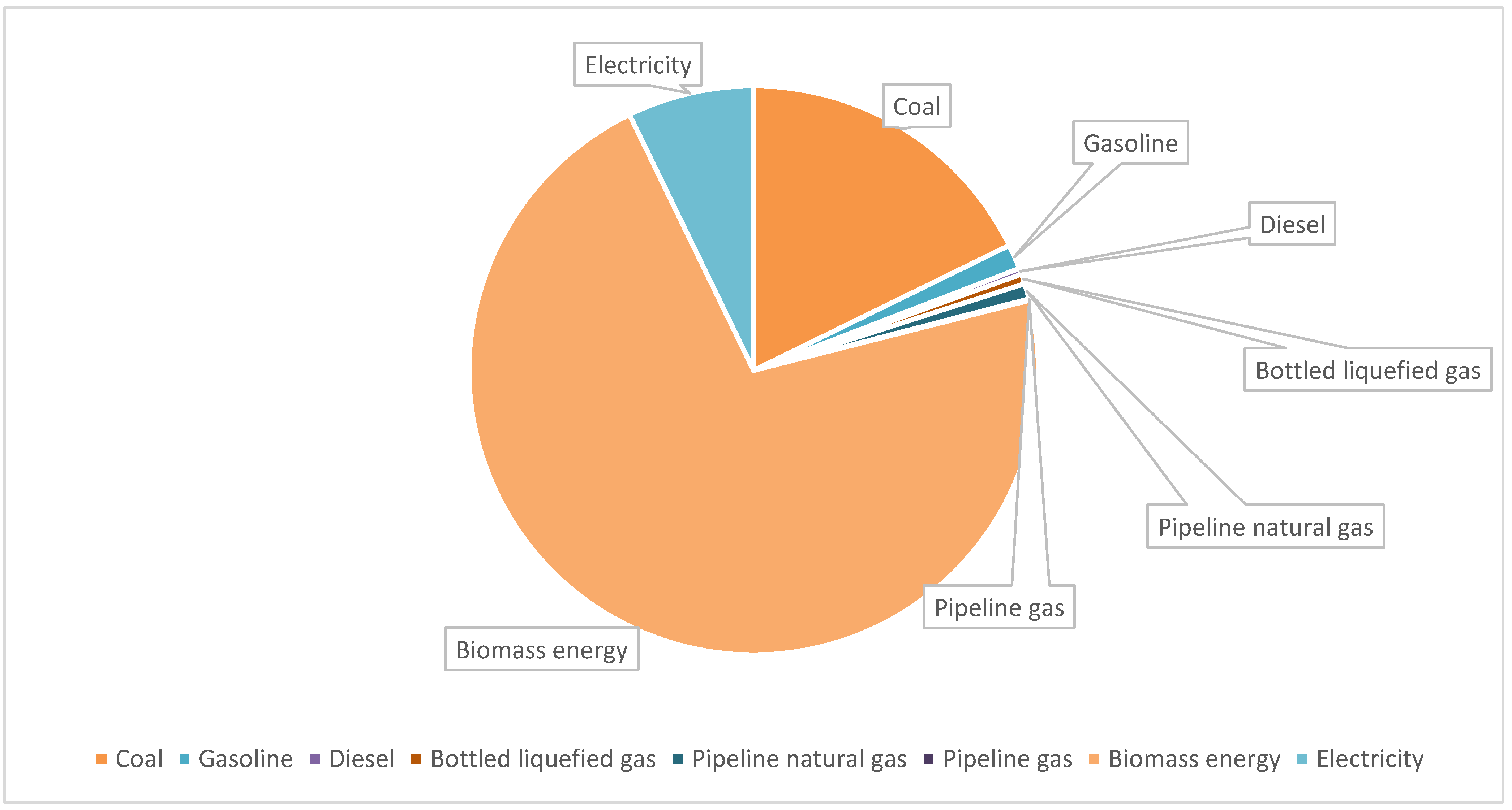
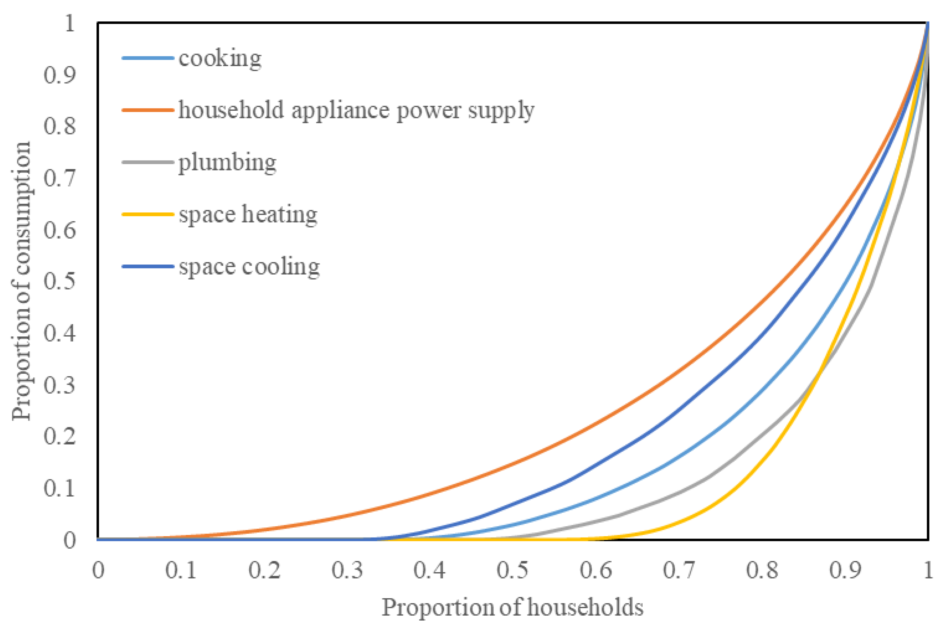
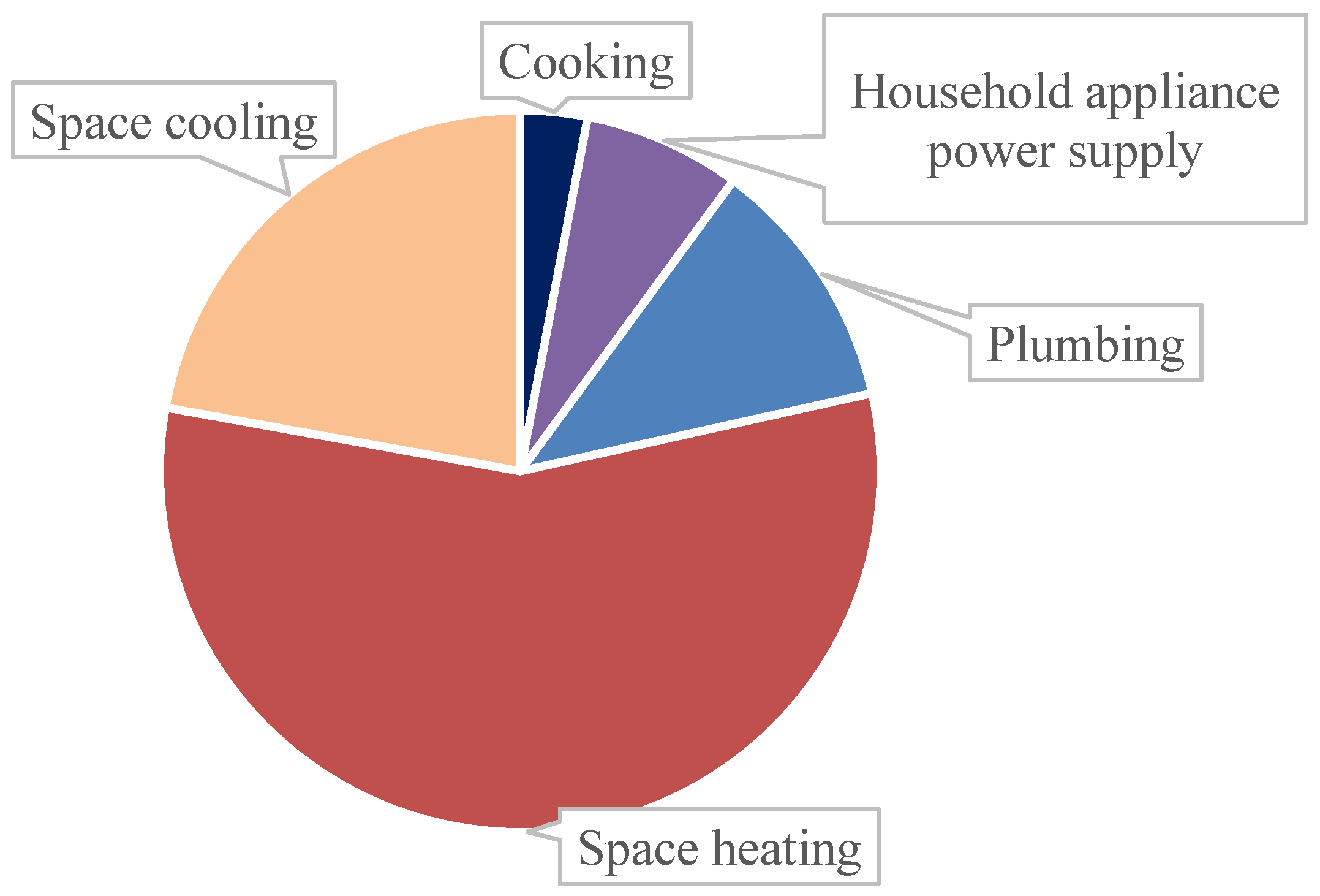
50]. This method is used to decompose Gini coefficient by energy types (coal, gasoline, diesel, bottled liquefied gas, pipeline natural gas, pipeline gas, biomass energy, electricity) and end-use activities (cooking, household appliance power supply, plumbing, space heating, and space cooling).
4.4. Decomposing Gini Coefficient by Urban–Rural Areas and Regions
The data can be divided by urban–rural and regional subgroups, and accordingly, the calculation of Gini coefficient can be further rearranged as below [
51]:
ni/n indicates the proportion of group i in a total population; wi indicates the proportion of group i in the total consumption; Gi indicates the Gini coefficient of group i; Gwithin indicates the difference contribution within group i; Gbetween indicates the difference contribution among groups; Goverlap indicates the difference intensity contribution among groups.
Intergroup difference contribution Gwithin implies the contribution of difference within the group i to the total difference; the intergroup difference contribution Gbetween implies the contribution of difference between each group to the total difference. The larger the number of groups, the greater a difference contribution among groups. The difference intensity contribution among groups, as known as the overlap effect, depends on the frequency and degree of overlap between the energy consumption of different groups. If the range of household energy consumption does not overlap, it will have a zero value. For example, if the highest power consumption of one group is lower than the lowest power consumption of another group, the overlap effect is equal to zero.
7. Energy-Consumption Differences in Urban–Rural Areas
In this section, gasoline, diesel, and pipeline gas were excluded from the analysis as the number of households using them was too small to accurately reflect urban–rural differences, thus six indicators were finally selected: coal, bottled liquefied gas, pipeline natural gas, biomass energy, electricity, and total energy consumption, which were all measured in standard coal equivalent unit (kgce).
7.1. Analysis Based on Gini Coefficient and Lorenz Curve
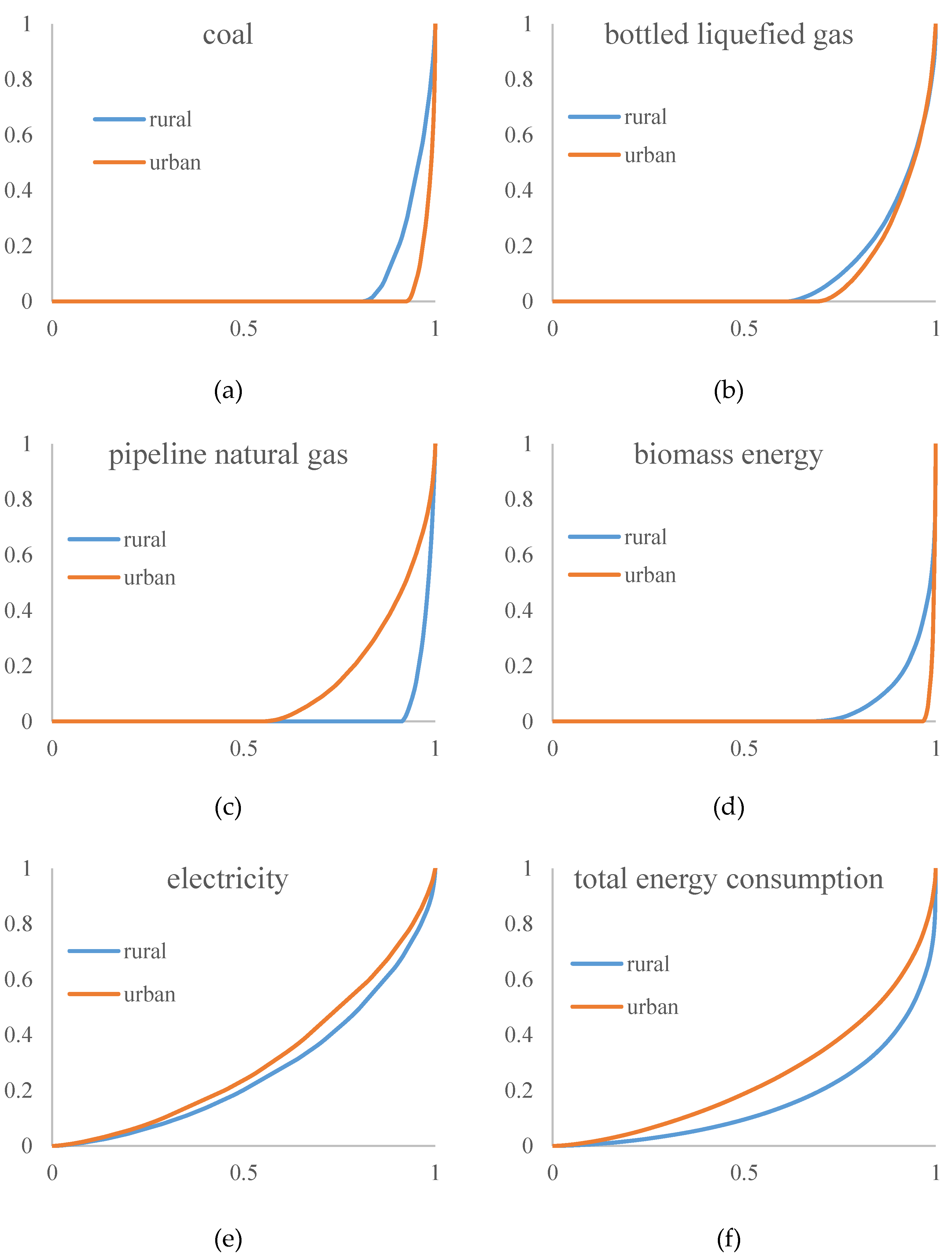
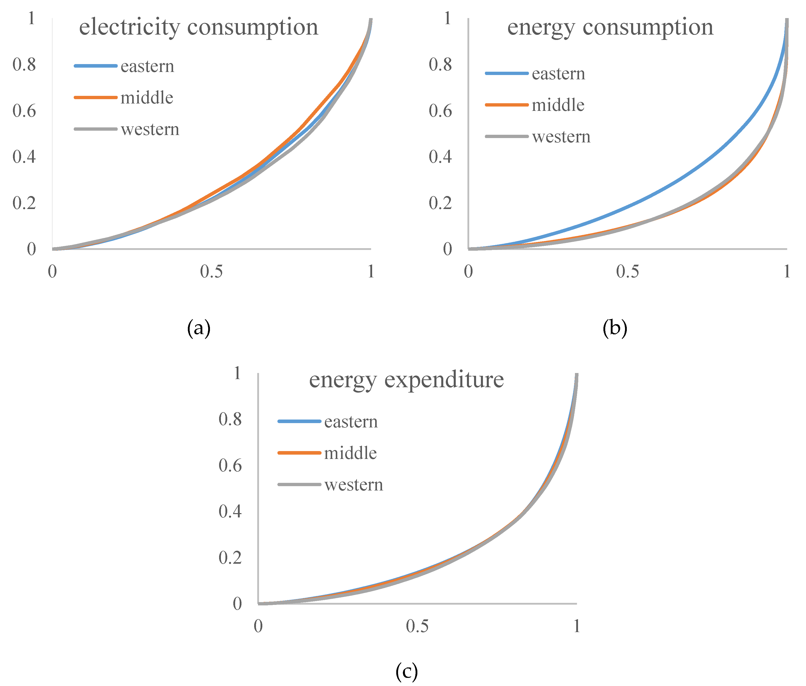
The Gini coefficients are calculated separately, and Lorenz curves are drawn for each indicator to visualize the differences. The results are shown in
Figure 5 and
Table 5, respectively.
The findings show that rural electricity consumption differences are slightly higher than that of urban users, but both are at a lower level. Compared to electricity consumption, total energy consumption shows a greater urban–rural difference, with its difference within rural areas being much greater than in urban areas. The difference between the urban and rural Lorenz curves for bottled liquefied gas is very minor. The overall Gini coefficients for both coal and biomass exceed 0.9, and because both have higher penetration rates in rural area, their Gini coefficients in rural area are both lower. Pipeline natural gas has a penetration rate of 45.19% in urban areas, yet only 8.79% in rural areas, resulting in greater intrarural difference than intraurban difference. It is a similar case for coal and biomass too. In addition,
Table 3 shows that the Lorenz asymmetry coefficients for coal, bottled liquefied gas, pipeline natural gas, and biomass energy are all less than 1, implying that these differences are mainly produced by many users with a low level of energy consumption.
7.2. Analysis Based on Decomposing Gini Coefficient
After studying the relationship between the overall Gini coefficient and the urban–rural Gini coefficient and further investigating the source of such a difference, the overall Gini coefficient is decomposed as below:
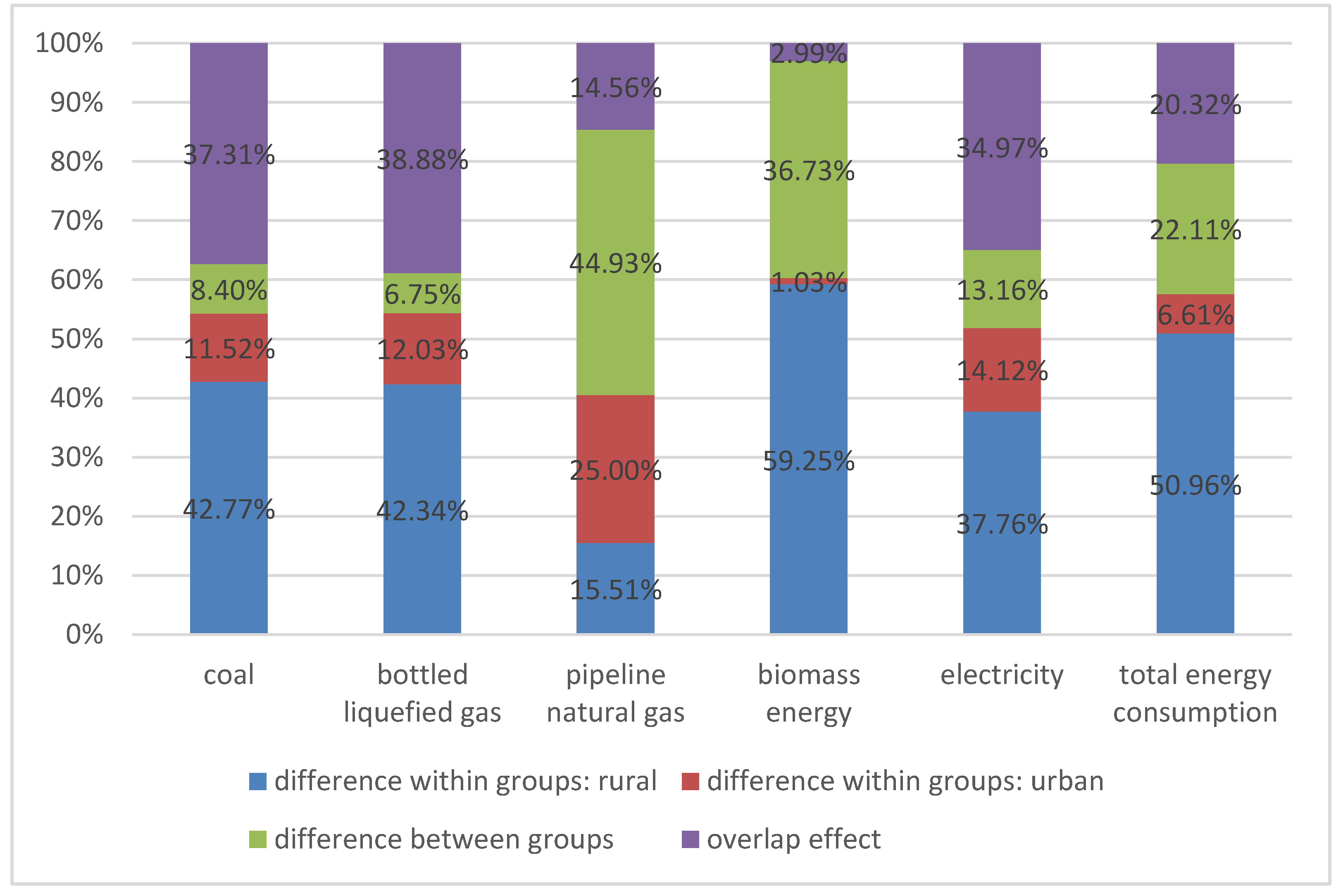
In
Figure 6, more than half of the total energy-consumption difference derives from within the rural areas. The structure of the sources of difference for coal, bottled liquefied gas, and electricity is very similar, all deriving primarily from intrarural household differences. The structure of differences in biomass energy reveals the most extreme urban–rural differences, because only an intensely small number of households use biomass energy in urban areas.
Pipeline natural gas is the only energy type wherein the contribution of intraurban difference is greater than the contribution of intrarural difference, because pipeline natural gas is used by nearly 50% of households in urban areas but just under 10% in rural areas, with urban consumption being more than three times greater than rural consumption. At the same time, the contribution of between-group difference of pipeline natural gas is 44.93%, the highest of the six indicators, indicating that there are significant differences in the household consumption of natural gas between rural and urban areas.
Comparing the six indicators horizontally, it can be found that, in addition to pipeline natural gas, internal differences in rural areas have always been the main cause of overall differences. In terms of differences between groups, the differences of pipeline natural gas and biomass energy are large. The urban–rural differences in coal, bottled liquefied gas, and electricity are all small, claiming that urban and rural households have no significant difference in the three types of energy consumption, and urban and rural factors are not the main factors affecting consumption. There have been an ocean of studies on the difference in energy consumption between urban and rural areas, but most of them are carried out from a macro perspective, such as Dong et al. (2018) [
26] and Fan et al. (2020) [
28]. More importantly, this section integrates urban–rural differences with intraurban differences and intrarural differences and has a more comprehensive discussion, revealing that the different energy types have different patterns in the relationship between differences within groups and differences between groups. Considering all above, it is evident that with further decomposition between urban and rural areas, new trends and features have emerged, in addition to the solid findings obtained by H1 and H2
. Therefore, H3a is confirmed, and this result implies the complex and dynamic feature of energy-consumption patterns in China.


