
A Design Procedure for Anchors of Floating Ocean Current Turbines on Weak Rock


Abstract
:1. Introduction
- Local water depth;
- Type of seabed;
- Installation complexity;
- Characteristics of the turbine;
- Transportation of the system components.
- (i)
- Determining the preliminary design of the anchor (geometry);
- (ii)
- Evaluating the structural capacity of the anchor; and
- (iii)
- Computing the geotechnical capacity of the anchor on rock.
2. Proposed Design Procedure
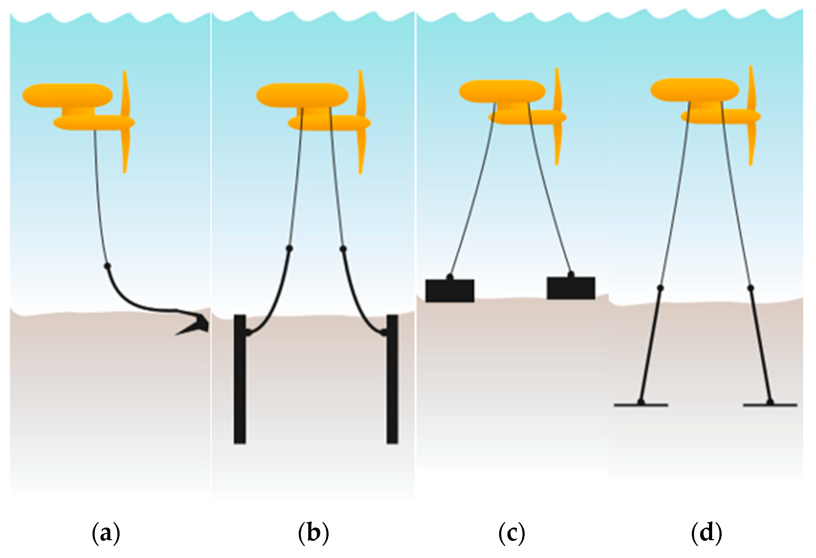
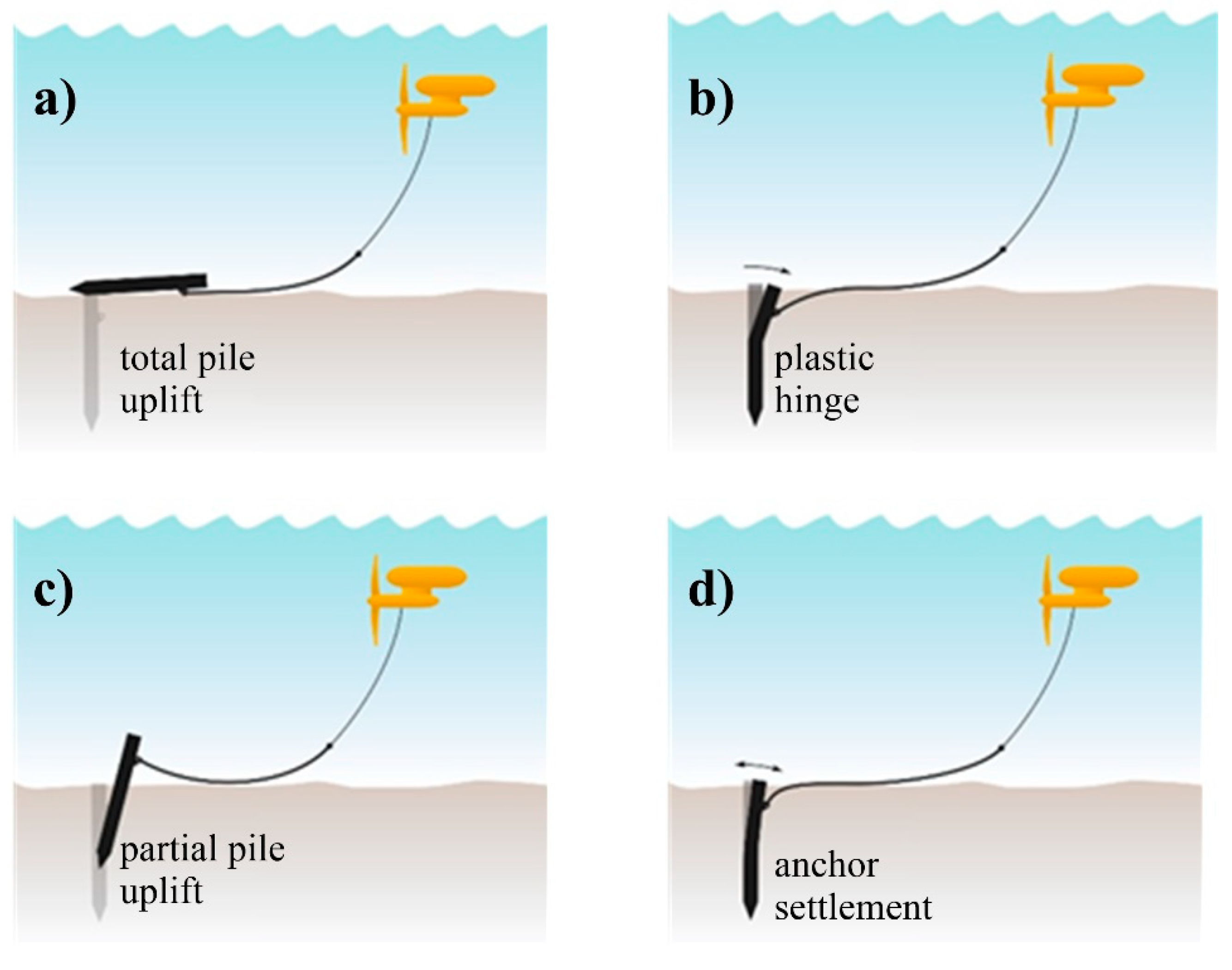
- Static equilibrium of the anchor is lost (whole or part), with a consequent failure mechanism, such as overturning, sliding, uplift. The case of a total pile uplift is shown in Figure 3a.
- Structural resistance is lost, leading to excessive yielding and the formation of a plastic hinge or cracks in concrete elements. Figure 3b shows a steel pile with a plastic hinge.
- Component fracture (for example, in the connections).
- Excessive displacements or rotations, leading to total, or partial, malfunction of the turbine. In Figure 3c, the pile has not moved completely, but the device will no longer generate electricity.
- Excessive vibration, limiting the performance of non-structural components.
- Differential settlements of the anchor, generating excessive rotation of the system. In Figure 3d, the back-and-forth movement of the pile lessens the stability and safety of the turbine.
2.1. Ultimate Limit State Design
2.1.1. Pile Anchors (PA)
Preliminary Design
- Initial parameters. The environmental and structural data for the design is collected, these are specific parameters from the deployment site and device such as: characteristics of the ocean current turbine, geotechnical parameters, and environmental loads, such as marine currents. The mechanical properties of the steel are also needed; for example, yield stress, , ultimate stress, , Young′s modulus, . The latter can be obtained from the design codes and technical documents of steel structures API RP 2A-LRFD [16].
- Pre-dimensioning of the diameter. A preliminary pile diameter is proposed, based on the designer’s experience or on practical recommendations.
- Pile wall thickness. The thickness of the pile, , is determined using the following Equation API RP2A-WSD [16]:where is the pile diameter in mm and is the thickness of the pile wall in mm.
- Embedded length. The embedded length, , is computed with the formula of Poulos and Davis [36]:where is the embedded length in m; is Young’s modulus of the steel, , is the second moment of area (see Appendix A), and is the horizontal coefficient of the subgrade reaction.
Structural Capacity
- 6.
- Axial capacity (structural). Anchors for floating structures are only loaded by tension stresses. The structural capacity to axial loads is determined, based on API RP 2A-LRFD [16]:where is the yield stress of the steel, , is the cross-sectional of the anchor, and is the resistance factor for axial tensile strength, which can be taken as 0.95 API RP 2A-LRFD [16].
- 7.
- Lateral capacity (structural). The shear capacity, , of the pile can be determined, using the following expressions [37]:withis the maximum value between Equations (6) and (7) and must not exceed 0.6 .The resistance factor for lateral strength, is 0.90 LRFD [37].
- 8.
- Revision of structural capacity. To satisfy the design requirements, the total force on the mooring system () must not exceed the axial () and lateral capacities ().It is worth mentioning that buckling does not occur in anchors for floating. However, it can be estimated by the Equations presented in DNV-OS-J101 [15]. If the above requirements are not fulfilled, the pile geometry must be modified, and the revision procedure restarted.
Geotechnical Capacity
- 9.
- Resistance of the pile shaft. The ultimate shaft resistance, , can be calculated using the following expression:where is the unit outside shaft friction and N is the number of layers.
- (a)
- Cohesionless Soil Interface
For piles in cohesionless soils, can be calculated with Equation (9) API RP2A-WSD [16]:where is the coefficient of lateral earth pressure, is the effective overburden pressure, is the friction angle between the soil and the pile wall, is the surface area of the pile shaft (see Appendix A), and is the limiting skin friction.Further information regarding the definition of , and can be found in [38].- (b)
- Cohesive Soil Interface
For piles in cohesive soils, , is calculated using the following expression [16]:where is the undrained shear strength, and is the adhesion factor.This factor is related to undrained shear strength, effective overburden pressure, and interface roughness [31].- (c)
- Chalk
The widely accepted guidance on pile design in chalk provided by CIRIA [29] suggests that the limiting skin friction varies between 30 kPa and 50 kPa for large- displacement, pre-formed piles in low to medium density chalk [39] defined the peak post-cyclic shear strength, , as:where is the steel-chalk interface friction coefficient, is the post peak internal soil friction coefficient (from cyclic simple shear), and is the undrained shear strength.- (d)
- Rock Socket Interface
A significant amount of research has been undertaken regarding the pile-rock interface for rock socket piles. The roughness and cleanliness of the rock socket are important factors in determining the pile-rock adhesion and have a significant influence on pile load capacity. The limiting skin friction for grouted rock sockets is often governed by the rock strength as follows:where is the adhesion factor, which depends on socket roughness but is generally taken as 0.1 for a smooth socket [29].
- 10.
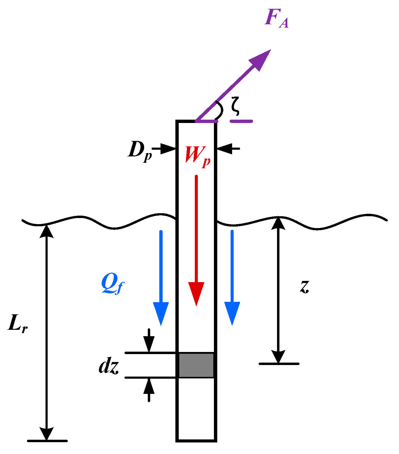
- Geotechnical capacity. The axial geotechnical capacity, , of piles driven into rock depends on the resistance of the pile shaft, , defined in Equations (8)–(12), and the submerged weight of the pile, (see Appendix A), given in Equation (A1). Figure 4 shows free-body diagram of the pile anchor.
- 11.
- Geotechnical design revision. The acting design loads on the pile, , must not exceed the geotechnical capacity, . Otherwise, the diameter must be reviewed and adjusted accordingly, followed by a re-evaluation of the anchor, starting the design procedure, from Step 3.
2.1.2. Dead Weight Anchors
Preliminary Design
- Initial parameters. The design criteria for DWAs are available in the literature as well as experimental design data [3,14,17]. In addition, the designer needs to gather the mechanical properties of the concrete, such as Young’s modulus, , and compressive strength, , among others. These parameters can be obtained from the concrete structure design codes and technical documents, for example, ACI 318-08 [41].
- Structural analysis. A structural analysis of the system is carried out, based on the loads obtained. From this analysis, the mechanical elements of the system are obtained: axial force, shear force, overturning moment, and displacements.
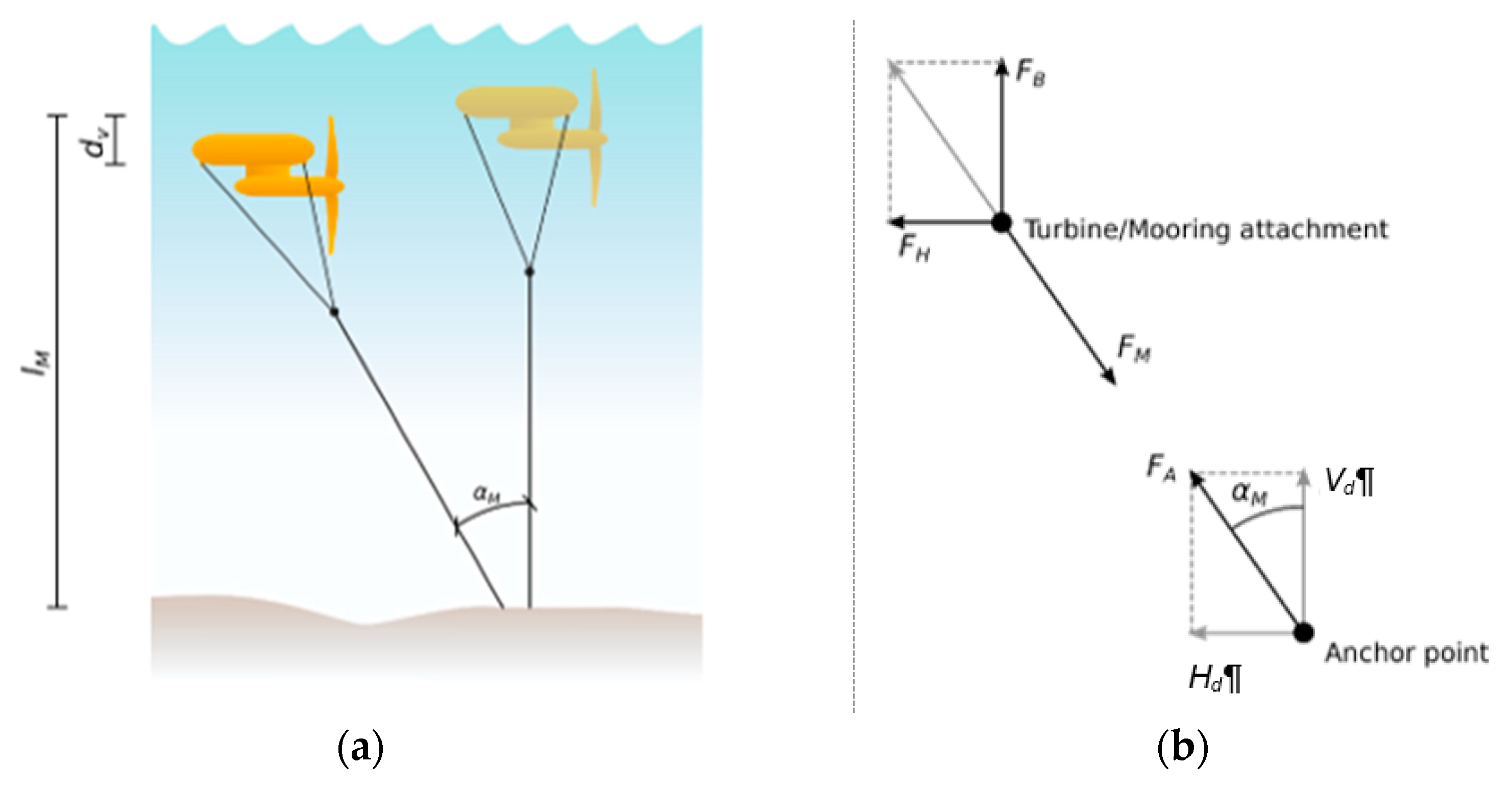
- Anchor weight. A preliminary anchor design is made. At this point, the Equations proposed by van Zwieten et al. [14] can be used. To resist sliding on cohesionless soils the required submerged weight, is calculated using the following Equation:where is the horizontal component of the anchor loading, is the angle of internal friction of the sediment, and is the vertical component of the anchor loading.
- 4.
- Anchor diameter.
- 5.
- Overturning moment. The overturning moment of the structure, , is determined based on following Equation:The load eccentricity , is determined using:
Geotechnical Capacity
- 6.
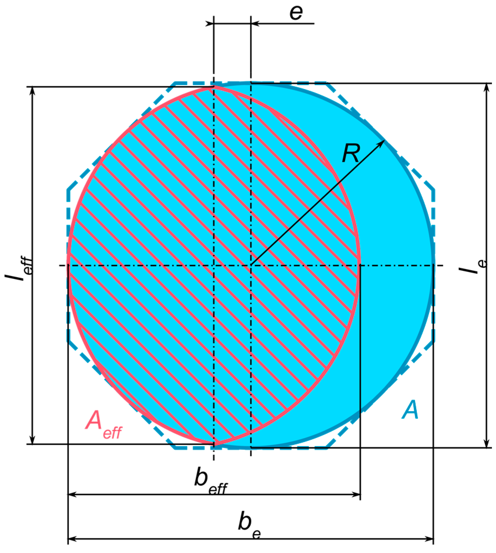
- Effective dimensions. To determine the bearing capacity, an effective base area is needed (see Appendix C). Bearing capacity: In fully drained conditions, the general formula below can be applied for the bearing capacity of a foundation with a horizontal base, resting on the soil surface:
- 7.
- Sliding capacity. The sliding capacity for drained conditions can be determined by the following Equation:In the case of undrained soils:
- 8.
- Design revision. The acting forces must be less than the resistant axial and sliding forces . If this condition is not fulfilled, the preliminary design is modified, and the design process started again.
Structural Capacity
- 9.
- Axial capacity (structural). The tensile capacity, , of the structure is determined using the following Equation ACI 318-08 [41]:
- 10.
- Lateral capacity (structural). The shear-resistant capacity, , of the anchor is determined using the following Equation [41]:
- 11.
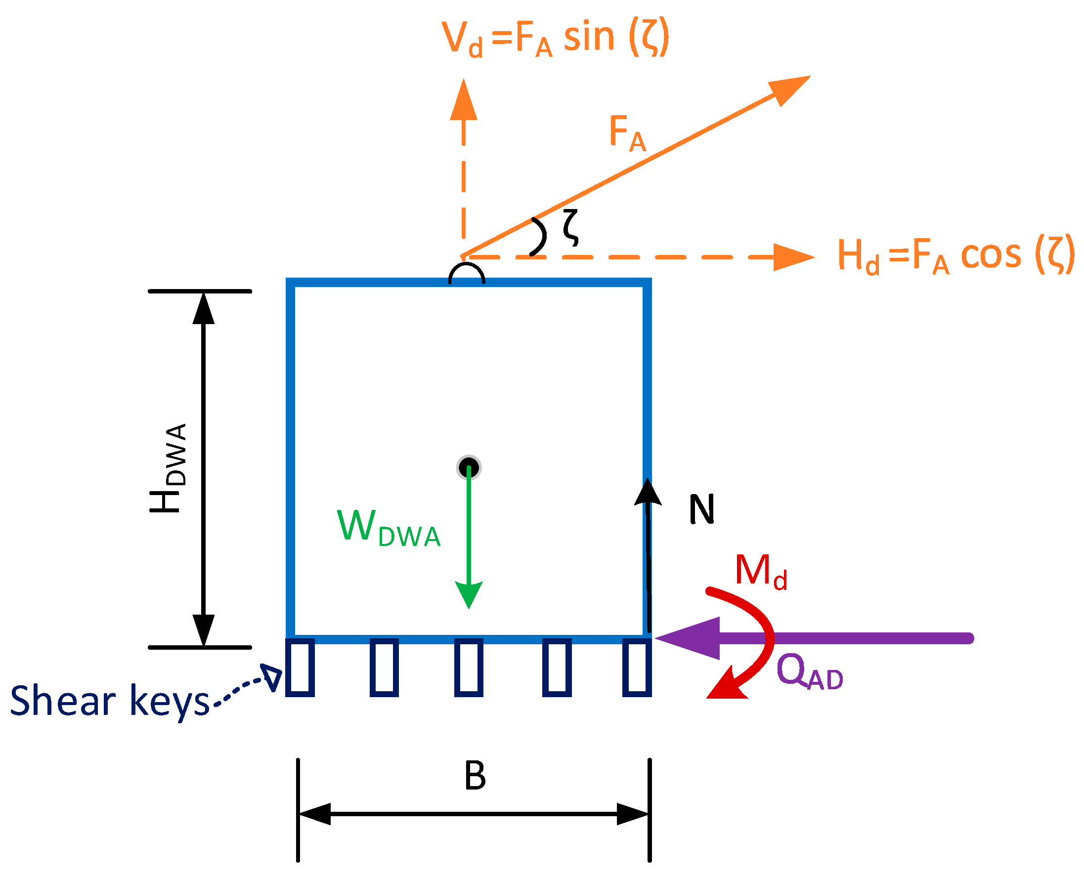
- Sliding capacity. The sliding capacity can be determined by (see Figure 5):
2.2. Service Limit State Design
2.2.1. Pile Anchors
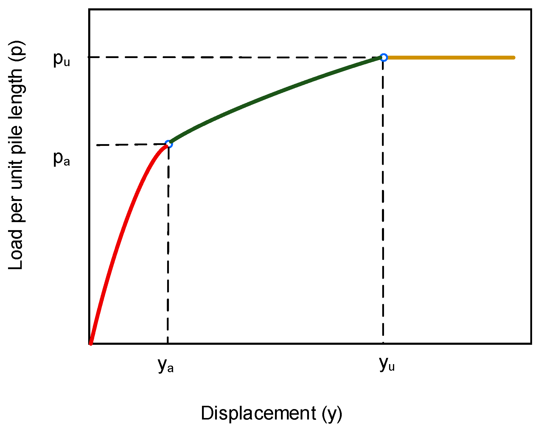
P–Y Curves
2.2.2. Deadweight Anchors
2.3. Fatigue Limit State Design
2.3.1. Fatigue Analyses
2.3.2. S–N Curves
Steel Anchors
Concrete Anchors
3. Application of the Design Procedure
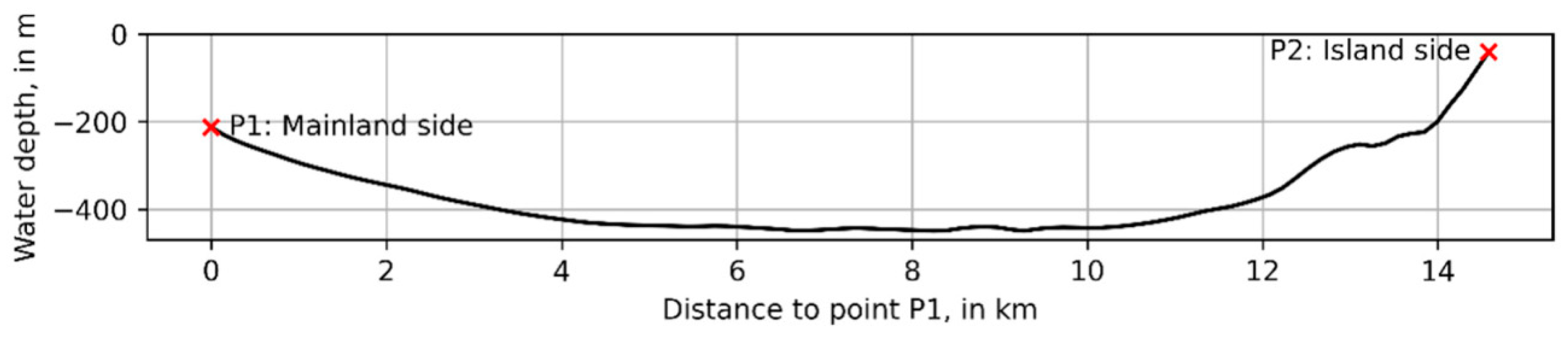
3.1. Case Study
3.2. Design Considerations
3.2.1. Environmental Interaction
3.2.2. Wave-Induced Velocity
3.2.3. Wind-Induced Velocity
3.2.4. Horizontal Force on the Mooring System
3.2.5. Total Force on the Mooring System
3.3. Design Results and Discussion
4. Conclusions and Recommendations
- (e)
- Both anchor designs showed satisfactory results based on the stipulations in the relevant design codes and technical documents. However, to guarantee this conclusion, it is necessary to carry out additional design tests.
- (f)
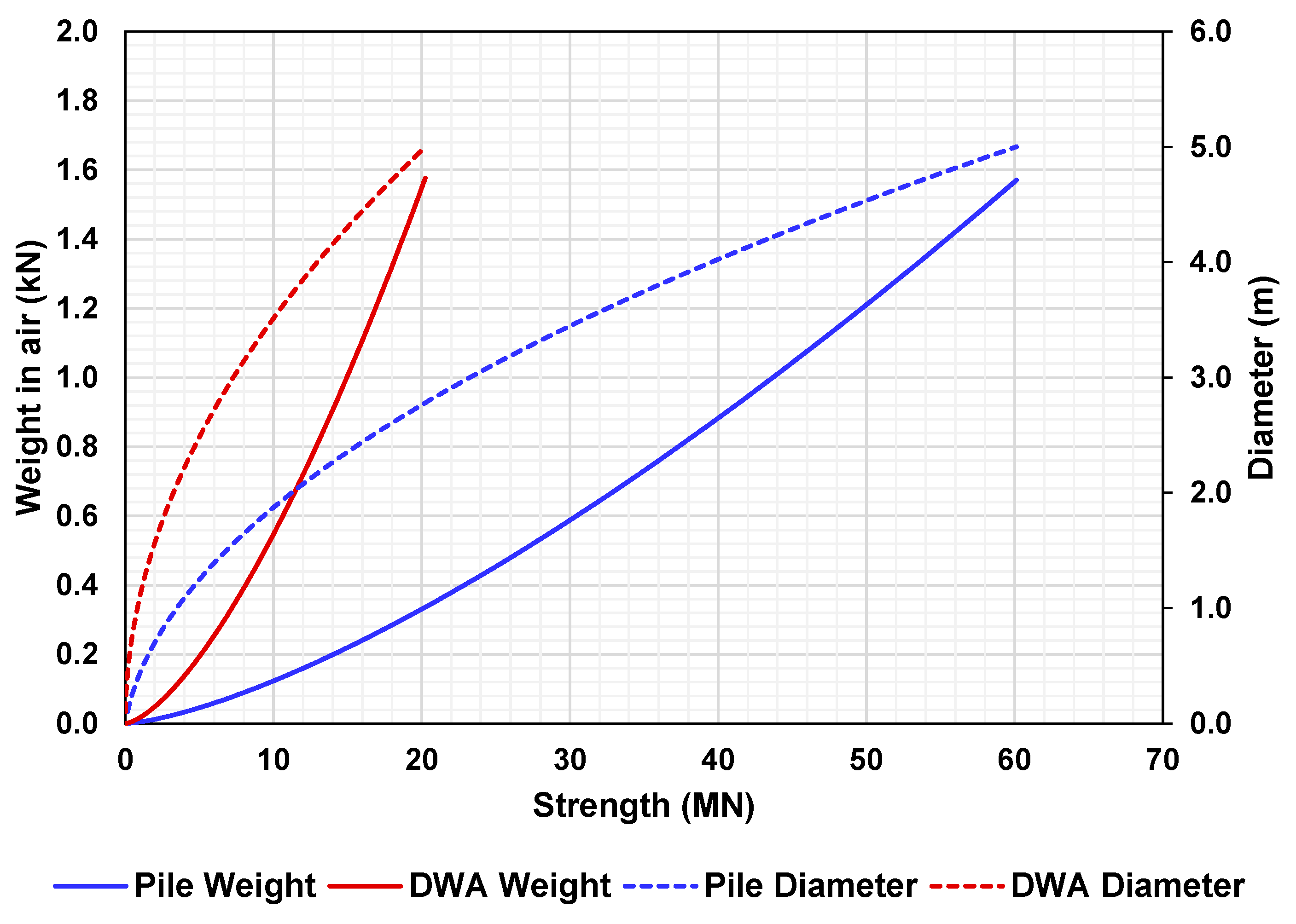
- For relatively small projects, DWAs are the better option. In larger projects, piles are more suitable, especially if the dimensions of the DWA mean that expensive transportation and installation equipment are required.
- (g)
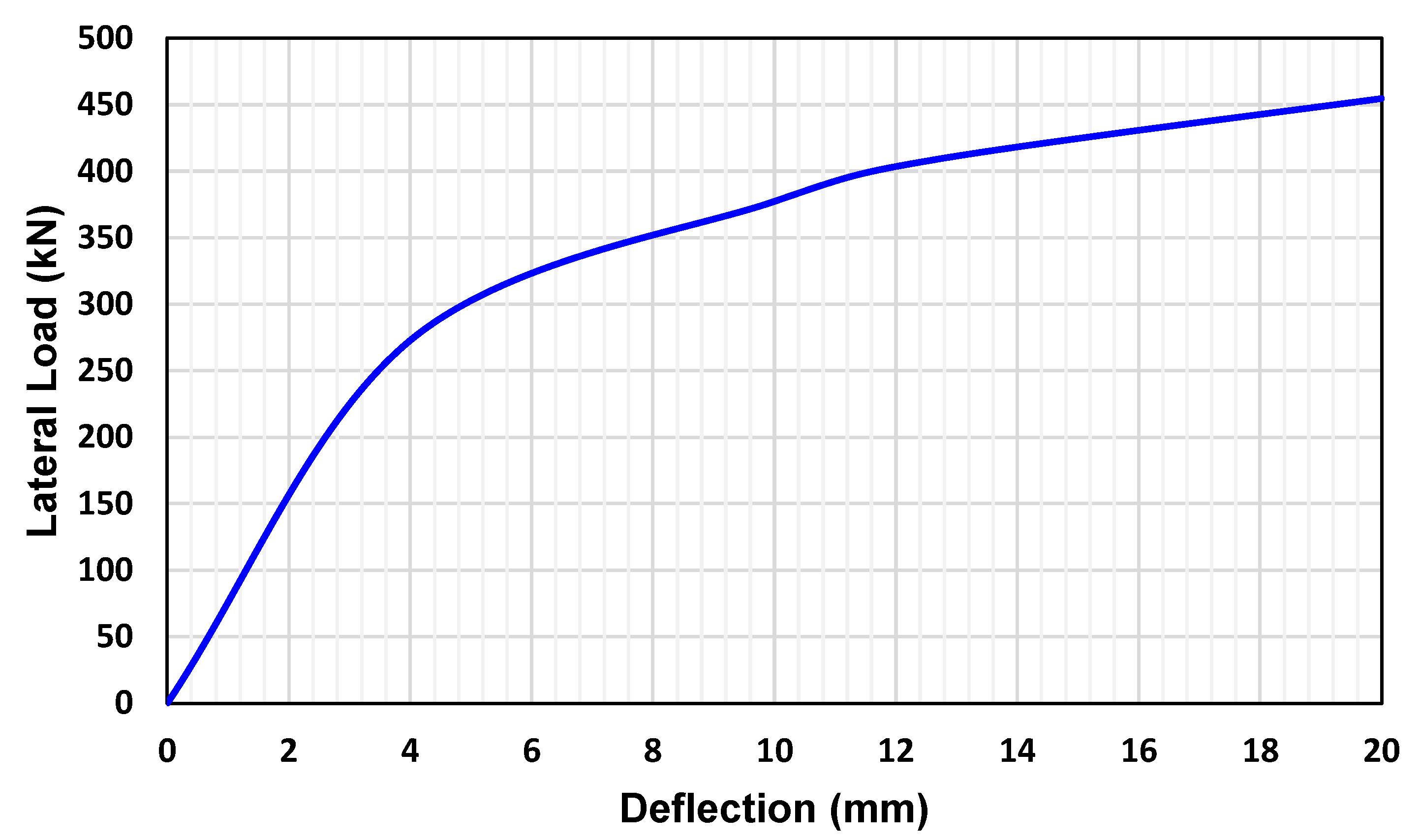
- The deflection presented in the pile satisfies the maximum permissible value corresponding to the recommendations indicated in the technical documents for marine structures design.
Author Contributions
Funding
Conflicts of Interest
Nomenclature
| Symbol | Description |
| undisturbed current speed | |
| wind induced velocity | |
| current velocity | |
| tidal velocity | |
| wave induced velocity | |
| parameter defined as 1.0 m | |
| effective area | |
| surface area of the pile shaft | |
| cross-sectional area of anchor | |
| area of rotor sweep | |
| type of cyclic stress factor | |
| extended lifetime factor | |
| drag coefficient of the rotor | |
| power coefficient | |
| pile diameter | |
| accumulated damage | |
| design wave height | |
| Young′s modulus of concrete | |
| Initial modulus of rock | |
| Young′s modulus of steel | |
| final load on the anchor | |
| required buoyancy force | |
| maximum theoretical drag | |
| load produced by the turbine chain | |
| resulting force on the mooring line | |
| critical strength | |
| ultimate stress | |
| yield stress | |
| height of the cylindrical anchor | |
| horizontal anchor loading | |
| wave height of the i-th block | |
| maximum height of the mooring line connection point above the base of the anchor | |
| area moment of inertia of the pile cross section | |
| passive earth pressure coefficient | |
| length of the cubical anchor | |
| embedment length | |
| overturning moment | |
| bearing resistance factor for drained conditions | |
| bearing resistance factor for undrained conditions | |
| normal force | |
| number of load cycles which would damage the structure under same load patterns as in the i-th block | |
| number of load cycles which would damage the structure under same load patterns as in the i-th block, considering extended design life | |
| axial structural capacity of DWA | |
| axial geotechnical capacity of pile | |
| axial structural capacity of DWA | |
| Axial structural capacity of pile | |
| sliding geotechnical capacity of DWA | |
| lateral geotechnical capacity of pile | |
| lateral geotechnical capacity of DWA | |
| Lateral structural capacity of pile | |
| sliding structural capacity of DWA | |
| ultimate shaft resistance | |
| period of service life | |
| reference period | |
| design wave period | |
| wave period corresponding to i-th block | |
| vertical anchor loading | |
| lateral capacity of a deadweight anchor with full-base keying skirts in cohesionless soil | |
| submerged weight of dead weight anchor | |
| submerged weight of each shear key | |
| submerged weight of pile | |
| depth to the bottom of the skirts | |
| Factor, directly related to intercept of log N-axis of S–N curve () | |
| effective dimensions | |
| design cohesion | |
| maximum permitted vertical deflection of the platform | |
| compressive strength of concrete | |
| limiting skin friction | |
| compressive strength of concrete for specific failure type in fatigue analysis | |
| peak post-cyclic shear strength | |
| normalized structural tensile strength of concrete (Table C1) DNV-OS-C502 | |
| inclination factor for undrained conditions | |
| , | inclination factors for drained conditions |
| constant, used in calculations of crack width (Table O3) DNV-OS-C502 | |
| dimensionless coefficient defined by Equation (A5) | |
| dimensionless coefficient in the range of 0.0005 and 0.00005 | |
| coefficient dependent on cross-sectional height | |
| length of the mooring | |
| dimensions defined in Appendix C | |
| effective dimensions in Appendix C | |
| horizontal coefficient of subgrade reaction of the soil | |
| denotes the number of load cycles in the i-th block | |
| number of shear keys | |
| effective overburden pressure at the level of the foundation-soil interface | |
| elastic lateral pile resistance | |
| relative probability of the i-block in fatigue analysis | |
| ultimate pile resistance | |
| embedment force of shear keys | |
| soil’s uniaxial unconfined strength | |
| , , | shape factors for drained conditions |
| shape factor for undrained conditions | |
| undrained shear strength | |
| design undrained strength assessed based on the shear strength profile | |
| pile wall thickness | |
| shear key thickness | |
| reference thickness | |
| design wind speed at 10 m height | |
| induced velocity | |
| one hour mean wind speed 10 m above MSL | |
| design ocean current | |
| design tidal current | |
| maximum and minimum horizontal velocity | |
| elastic limit pile deflection | |
| accumulated pile deflection | |
| initial pile deflection | |
| ultimate pile deflection | |
| effective angle of the mooring | |
| strength reduction factor | |
| submerged specific weight of the anchor material (concrete) | |
| specific weight of the anchor shear keys | |
| specific weight of structural steel | |
| submerged unit weight of soil | |
| specific weight of water | |
| wave amplitude | |
| water density | |
| initial pile rotation | |
| pile’s accumulated deflection rotation | |
| principal tensile stress | |
| edge stress due to bending alone (positive tension) | |
| stress due to axial force (positive tension) | |
| maximum stress due to cyclic load for i-th block in fatigue analysis | |
| minimum stress due to cyclic load for i-th block in fatigue analysis | |
| parameter defined by Equation (A26) | |
| tangent of the friction angle at depth . | |
| resistance factor for axial tensile strength (0.95) | |
| resistance factor for shear strength for concrete anchor (0.75) | |
| resistance factor for shear strength for steel anchor (0.9) | |
| cross-section height | |
| friction angle between the soil and the pile wall | |
| minimum anchor width/diameter | |
| coefficient of lateral earth pressure | |
| number of layers | |
| rock quality designation | |
| cohesion of the soil | |
| local water depth | |
| eccentricity of the vertical force | |
| unit outside shaft friction | |
| gravitational acceleration | |
| total number of blocks | |
| exponent on thickness, for fatigue analysis | |
| negative inverse slope of S–N curve | |
| load per pile length unit | |
| material thickness | |
| pile deflection | |
| depth below MSL | |
| cyclic load range for i-th block in fatigue analysis | |
| adhesion factor | |
| steel-chalk interface friction coefficient | |
| angle formed between the turbine chain and the anchor | |
| wave number | |
| friction coefficient | |
| modification factor that reflecting the reduced mechanical properties of concrete, ACI 318-08 | |
| pile rotation | |
| dimensionless parameter | |
| angular frequency | |
| parameter defined based onthe type of concrete | |
| internal friction angle of the sediment | |
| post peak internal soil friction coefficient |
Appendix A
Appendix B

| Parameter | Symbol | Unit |
|---|---|---|
| Uniaxial unconfined strength | kPa | |
| Strength reduction factor | - | |
| Dimensionless coefficient in the range of 5 × 10⁻⁴ and 5 × 10⁻⁵ | - | |
| Initial modulus of the intact rock | kPa |
Appendix C

References
- Astariz, S.; Vazquez, A.; Iglesias, G. Evaluation and comparison of the levelized cost of tidal, wave, and offshore wind energy. J. Renew. Sustain. Energy 2015, 7, 053112. [Google Scholar] [CrossRef]
- Vazquez, A.; Iglesias, G. Capital costs in tidal stream energy projects—A spatial approach. Energy 2016, 107, 215–226. [Google Scholar] [CrossRef] [Green Version]
- Bhattacharya, S. Design of Foundations for Offshore Wind Turbines; John Wiley & Sons: Chichester, UK, 2019; Volume 1, ISBN 9788578110796. [Google Scholar]
- Starling, M.; Scott, A.; Parkinson, R. Foundations and Moorings for Tidal Stream Systems; BMT Cordah Limited: London, UK, 2009. [Google Scholar]
- Zhou, Z.; Benbouzid, M.; Charpentier, J.-F.; Scuiller, F.; Tang, T. Developments in large marine current turbine technologies—A review. Renew. Sustain. Energy Rev. 2017, 71, 852–858. [Google Scholar] [CrossRef]
- Meggitt, D.J.; Jackson, E.; Machin, J.; Taylor, R. Marine micropile anchor systems for marine renewable energy applications. In Proceedings of the 2013 MTS/IEEE—San Diego an Ocean Common, San Diego, CA, USA, 23–27 September 2013. [Google Scholar]
- Cresswell, N.; Hayman, J.; Kyte, A.; Hunt, A.; Jeffcoate, P. Anchor Installation for the Taut Moored Tidal Platform PLAT-O. In Proceedings of the 3rd Asian Wave Tidal Energy Conference, Singapore, Singapore, 24–28 October 2016; pp. 1–8. [Google Scholar]
- Ma, K.-T.; Luo, Y.; Kwan, T.; Wu, Y.B.T. Mooring System Engineering for Offshore Structures, 1st ed.; Gulf Professional Publishing: Houston, TX, USA, 2019; ISBN 9780128185513. [Google Scholar]
- Hernández-Fontes, J.V.; Felix, A.; Mendoza, E.; Cueto, Y.R.; Silva, R. On the Marine Energy Resources of Mexico. J. Mar. Sci. Eng. 2019, 7, 191. [Google Scholar] [CrossRef] [Green Version]
- Alcérreca-Huerta, J.C.; Encarnacion, J.I.; Ordoñez-Sánchez, S.; Callejas-Jiménez, M.; Barroso, G.G.D.; Allmark, M.; Mariño-Tapia, I.; Casarín, R.S.; O’Doherty, T.; Johnstone, C.; et al. Energy Yield Assessment from Ocean Currents in the Insular Shelf of Cozumel Island. J. Mar. Sci. Eng. 2019, 7, 147. [Google Scholar] [CrossRef] [Green Version]
- Graniel, J.B.; Fontes, J.; Garcia, H.; Silva, R. Assessing Hydrokinetic Energy in the Mexican Caribbean: A Case Study in the Cozumel Channel. Energies 2021, 14, 4411. [Google Scholar] [CrossRef]
- Muckelbauer, G. The shelf of Cozumel, Mexico: Topography and organisms. Facies 1990, 23, 201–239. [Google Scholar] [CrossRef]
- Taylor, R.J. Interaction of Anchors with Soil and Anchor Design; Naval Facilities Engineering Command: Port Hueneme, CA, USA, 1982; ISBN 9788578110796. [Google Scholar]
- Vanzwieten, J.H.; Seibert, M.G.; Ellenrieder, K. Von Anchor selection study for ocean current turbines. J. Mar. Eng. Technol. 2014, 13, 59–73. [Google Scholar] [CrossRef]
- Det Norske Veritas. DNV-OS-J101 Design of Offshore Wind Turbine Structures; Det Norske Veritas: Høvik, Norway, 2014. [Google Scholar]
- American Petroleum Institute. API RP2A-WSD Recommended Practice for Planning, Designing and Constructing Fixed Offshore Platforms—Working Stress Design; American Petroleum Institute: Washington, DC, USA, 2002. [Google Scholar]
- Arany, L.; Bhattacharya, S.; Macdonald, J.; Hogan, S. Design of monopiles for offshore wind turbines in 10 steps. Soil Dyn. Earthq. Eng. 2017, 92, 126–152. [Google Scholar] [CrossRef] [Green Version]
- McCarron, W. Deepwater Foundations and Pipeline Geomechanics, 1st ed.; J. Ross Publishing: Fort Lauderdale, FL, USA, 2011; ISBN 9781604270099. [Google Scholar]
- Bai, Y.; Jin, W.-L. Marine Structural Design, 2nd ed.; Elsevier: Oxford, UK, 2015; ISBN 9780080999975. [Google Scholar]
- El-Reedy, M.A. Marine Structural Design Calculations, 1st ed.; Butterworth-Heinemann: Oxford, UK, 2015; ISBN 9780080999876. [Google Scholar]
- Gaythwaite, J.W. Design of Marine Facilities, 3rd ed.; American Society of Civil Engineers: Reston, VA, USA, 2016; ISBN 9780784414309. [Google Scholar]
- Fleming, K.; Weltman, A.; Randolph, M.; Elson, K. Piling Engineering; CRC Press: London, UK, 2008; ISBN 9780415266468. [Google Scholar]
- Ferrero, A.; Migliazza, M.; Roncella, R.; Tebaldi, G. Analysis of the failure mechanisms of a weak rock through photogrammetrical measurements by 2D and 3D visions. Eng. Fract. Mech. 2008, 75, 652–663. [Google Scholar] [CrossRef]
- Dobereiner, L.; De Freitas, M.H. Geotechnical properties of weak sandstones. Geotechnique 1986, 36, 79–94. [Google Scholar] [CrossRef]
- Reese, L.C. Analysis of Laterally Loaded Piles in Weak Rock. J. Geotechnol. Geoenviron. Eng. 1997, 123, 1010–1017. [Google Scholar] [CrossRef]
- Goodman, R.E. Introduction to Rock Mechanics, 2nd ed.; John Wiley & Sons: New York, NY, USA, 1980; ISBN 9780471812005. [Google Scholar]
- Abbs, A.F. Lateral Pile Analysis in Weak Carbonate Rocks. In Proceedings of the Conference on Geotechnical Practice in Offshore Engineering, Austin, TX, USA, 27–29 April 1983; ASCE: Austin, TX, USA, 1983; pp. 546–556. [Google Scholar]
- Carter, J.P.; Kulhawy, F.H. Closure to “Analysis of Laterally Loaded Shafts in Rock” by John P. Carter and Fred H. Kulhawy (June, 1992, Vol. 118, No. 6). J. Geotechnol. Eng. 1993, 119, 2018–2020. [Google Scholar] [CrossRef]
- Gannon, J.A.; Masterton, G.G.T.; Wallace, W.A.; Wood, D.M. Piled Foundations in Weak Rock; Construction Industry Research and Information Association (CIRIA): London, UK, 1999. [Google Scholar]
- Zhang, L.; Ernst, H.; Einstein, H.H. Nonlinear Analysis of Laterally LoadedRock-Socketed Shafts. J. Geotechnol. Geoenviron. Eng. 2000, 126, 955–968. [Google Scholar] [CrossRef]
- Irvine, J.; Terente, V.; Lee, L.; Comrie, R. Driven pile design in weak rock. In Frontiers in Offshore Geotechnics III—Proceedings of the 3rd International Symposium on Frontiers in Offshore Geotechnics, Oslo, Norway, 10–12 June 2015; CRC Press: London, UK, 2015; pp. 569–574. ISBN 9781138028500. [Google Scholar]
- International Electrotechnical Commission. IEC 62600-10 Marine Energy—Wave, Tidal and Other Water (IEC, Current Converters—Part 10: Assessment of Mooring System for Marine Energy Converters); International Electrotechnical Commission: Geneva, Switzerland, 2015; ISBN 9782832224311. [Google Scholar]
- Das, B.M.; Sivakugan, N. Principles of Foundation Engineering, 9th ed.; Cengage Learning, Inc.: Boston, MA, USA, 2019; ISBN 9781337705035. [Google Scholar]
- Det Norske Veritas. DNV-RP-C203 Fatigue Design of Offshore Steel Structures; Det Norske Veritas: Høvik, Norway, 2014. [Google Scholar]
- Det Norske Veritas. DNV-OS-C502 Offshore Concrete Structures; Det Norske Veritas: Høvik, Norway, 2010. [Google Scholar]
- Poulos, H.G.; Davis, E.H. Pie Foundation Analysis and Design; John Wiley and Sons: New York, NY, USA, 1990; ISBN 0894644491. [Google Scholar]
- American Institute of Steel Construction (AISC). LRFD Load and Resistance Factor. Design Specification for Structural Steel Buildings; American Institute of Steel Construction: Chicago, IL, USA, 1999. [Google Scholar]
- Tomlinson, M.; Woodward, J. Pile Design and Construction Practice, 6th ed.; CRC Press: Boca Raton, FL, USA, 2015; ISBN 9781466592643. [Google Scholar]
- Carrington, T.; Li, G.; Rattley, M. A new assessment of ultimate unit friction for driven piles. In Proceedings of the 15th European Conference on Soil Mechanics and Geotechnical Engineering, Athens, Greece, 12–15 September 2011; Anagnostopoulos, A., Pachakis, M., Tsatsanifos, C., Eds.; IOS Press: Amsterdam, NY, USA, 2011; pp. 825–830. [Google Scholar]
- Gabr, M.A.; Borden, R.H.; Cho, K.H.; Clark, S.C.; Nixon, J.B. P-y Curves for Laterally Loaded Drilled Shafts Embedded in Weathered Rock; Department of Civil Engineering North Carolina State University: Raleigh, NC, USA, 2002. [Google Scholar]
- American Concrete Institute. ACI 318-08 Building Code Requirements for Structural Concrete and Commentary; American Concrete Institute: Farmington Hills, MI, USA, 1999; Volume 1, ISBN 9781942727118. [Google Scholar]
- Butterfield, R.; Gottardi, G. A complete three-dimensional failure envelope for shallow footings on sand. Geotechnique 1994, 44, 181–184. [Google Scholar] [CrossRef]
- Tistel, J.; Eiksund, G.R.; Hermstad, J.; Bye, A.; Athanasiu, C. Gravity Based Structure foundation design and optimization opportunities. In Proceedings of the Twenty-fifth International Ocean and Polar Engineering Conference, Kailua-Kona, HI, USA, 21–26 June 2015; pp. 772–779. [Google Scholar]
- Matlock, H. Correlations for design of laterally loaded piles in soft clay. In Proceedings of the Second Annual Offshore Technology Conference, Houston, TX, USA, 22–24 April 1970. [Google Scholar]
- Kallehave, D.; Thilsted, C.L.; Liingaard, M.A. Modification of the API p-y Formulation of Initial Stiffness of Sand. In Proceedings of the Offshore Site Investigation and Geotechnics: Integrated Technologies—Present and Future; Society of Underwater Technology: London, UK, 2012; p. 8. [Google Scholar]
- O’Neill, M.W.; Murchison, J.M. An Evaluation of p-y Relationships in Sands; Report No. GT-DF02-83; Department of Civil Engineering, University of Houston: Houston, TX, USA, 1983. [Google Scholar]
- Winkler, E. Die Lehre von der Elasticitaet und Festigkeit: Mit besonderer Rucksicht auf ihre Anwendung in der Technik; H. Dominicus: Prague, Czech Republic, 1868. [Google Scholar]
- Wesselink, B.D.; Murff, J.D.; Randolph, M.F.; Nunez, I.L.; Hyden, A.M. Analysis of Centrifuge Model Test Data from Laterrally Loaded Piles in Calcareous Sand; CRC Press: London, UK, 1988; pp. 261–270. ISBN 9781003211433. [Google Scholar]
- Williams, A.F.; Dunnavant, T.W.; Anderson, S.; Equid, D.W.; Hyden, A.M. The performance and analysis of lateral load tests on 356 mm dia piles in reconstituted calcareous sand. In Engineering for Calcareous Sediments; CRC Press: London, UK, 1988; pp. 271–280. ISBN 9781003211433. [Google Scholar]
- Dyson, G.J.; Randolph, M.F. Monotonic lateral loading of piles in calcareous sand. J. Geotechnol. Geoenviron. Eng. 2001, 127, 346–352. [Google Scholar] [CrossRef]
- Fragio, A.G.; Santiago, J.L.; Sutton, V.J.R. Load tests on grouted piles in rock. In Proceedings of the Annual Offshore Technology Conference, Houston, TX, USA, 6–9 May 1985; pp. 93–104. [Google Scholar]
- Turner, J. Rock-Socketed Shafts for Highway Structure Foundations, 1st ed.; Transportation Research Board of the National Academies: Laramie, WY, USA, 2006. [Google Scholar]
- Liang, R.; Yang, K.; Nusairat, J. p-y Criterion for Rock Mass. J. Geotechnol. Geoenviron. Eng. 2009, 135, 26–36. [Google Scholar] [CrossRef]
- Zdravkovic, L.; Taborda, D.; Potts, D.; Jardine, R.; Sideri, M.; Schroeder, F.; Byrne, B.; McAdam, R.; Burd, H.; Houlsby, G.; et al. Numerical modelling of large diameter piles under lateral loading for offshore wind applications. In Frontiers in Offshore Geotechnics III—Proceedings of the 3rd International Symposium on Frontiers in Offshore Geotechnics, Oslo, Norway, 10–12 June 2015; CRC Press: London, UK, 2015; pp. 569–574. ISBN 9781138028500. [Google Scholar] [CrossRef]
- Byrne, B.; Mcadam, R.; Burd, H.; Houlsby, G.; Martin, C.; Gavin, K.; Doherty, P.; Igoe, D.; Taborda, D.M.G.; Potts, D.; et al. Field testing of large diameter piles under lateral loading for offshore wind applications Field testing of large diameter piles under lateral loading for offshore wind applications. In Proceedings of the XVI ECSMGE Geotechnical Engineering for Infrastructure and Development, Edinburgh, UK, 13–17 September 2015; pp. 1255–1260. [Google Scholar]
- Ashour, M.; Norris, G.; Pilling, P. Lateral Loading of a Pile in Layered Soil Using the Strain Wedge Model. J. Geotechnol. Geoenviron. Eng. 1998, 124, 303–315. [Google Scholar] [CrossRef]
- Det Norske Veritas. DNV GL-ST-0126 Support Structures for Wind Turbines; Det Norske Veritas: Høvik, Norway, 2016. [Google Scholar]
- Harris, C.R.; Millman, K.J.; van der Walt, S.J.; Gommers, R.; Virtanen, P.; Cournapeau, D.; Wieser, E.; Taylor, J.; Berg, S.; Smith, N.J.; et al. Array programming with NumPy. Nature 2020, 585, 357–362. [Google Scholar] [CrossRef] [PubMed]
- International Electrotechnical Commission. IEC 62600-2 Marine Energy—Wave, Tidal and Other Water Current Converters—Part 2: Design Requirements for Marine Energy Systems; International Electrotechnical Commission: Geneva, Switzerland, 2016; ISBN 9782832235805. [Google Scholar]
- Dynamic Systems Analysis ProteusDS Manual v2.29.2. 2016. Available online: https://dsaocean.com/downloads/documentation/ProteusDS2015Manual.pdf. (accessed on 1 July 2021).
- Dhanak, M.R.; Xiros, N.I. Springer Handbook of Ocean Engineering; Springer: Trento, Italy, 2016; ISBN 9783319166490. [Google Scholar]
- Betz, A. Das Maximum der Theoretisch Möglichen Ausnutzung des Windes durch Windmotoren. In Zeitschrift für das Gesamte Turbinenwes; R. Oldenbourg: Munich, Germany, 1920; p. 20. [Google Scholar]
- Clarke, J.; Grant, A.; Connor, G.; Johnstone, C. Development and in-sea performance testing of a single point mooring supported contra-rotating tidal turbine. In Proceedings of the International Conference on Offshore Mechanics and Arctic Engineering—OMAE, Honolulu, Hawaii, USA, 31 May–5 June 2009; Volume 4, pp. 1065–1073. [Google Scholar]
- Ivashov, A. SMath Studio (Versión 0.99.7030). Available online: https://en.smath.com/view/SMathStudio/summary (accessed on 1 July 2021).
- Doherty, J.P. Lateral Analysis of Piles User Manual v 2.0. 2020. Available online: www.geocalcs.com/lap. (accessed on 1 July 2021).
| Type of Soil | Reference for P–Y Curves |
|---|---|
| Calcareous | Wesselink et al. [48] |
| Williams et al. [49] | |
| Dyson and Randolph [50] | |
| Weak rock | Reese [25] |
| Weak carbonate rock | Abbs [27] |
| Weak calcareous claystone | Fragio et al. [51] |
| Strong rock | Turner [52] |
| Massive rock | Liang et al. [53] |
| Parameter | Symbol | Value | Unit |
|---|---|---|---|
| Structural Steel (A36) | |||
| Yield stress | 25 | MPa | |
| Tensile strength | 400 | MPa | |
| Modulus of elasticity of steel | 200 | GPa | |
| Specific weight | 7860 | kN m−3 | |
| Structural concrete | |||
| Concrete Compressive Strength | 35 | MPa | |
| Specific weight | 23.6 | kN m−3 | |
| Limestone | |||
| Specific weight | 26.5 | kN m−3 | |
| Coefficient of subgrade reaction | 80 | MN m−3 | |
| Sand | |||
| Internal friction angle of the soil | 30 | degrees | |
| Specific weight | 17 | kN m−3 | |
| Effective overburden pressure | 10 | kN m−2 | |
| Material factor | 1.2 | - | |
| Friction coefficient | 0.5 | - | |
| Turbine | |||
| Rotor diameter | 1 | m | |
| Drag coefficient | 8/9 | - | |
| Length of mooring line | 20 | m | |
| Allowed vertical deflection | 0.5 | m | |
| Design depth of operation | 10 | m | |
| Environment | |||
| Design ocean current | 2.5 | m s−1 | |
| Design tidal current | 0 | m s−1 | |
| Design wave height | 7 | m | |
| Design wave period | 9 | s | |
| Design wind speed at 10 m height | 15 | m s−1 | |
| Local water depth | 30 | m | |
| Water density | 1025 | kg m−3 |
| Parameter | Symbol | Value | Unit | Equation |
|---|---|---|---|---|
| Load Design | ||||
| Final load of system | 100.0 | kN | (48) | |
| Pile | ||||
| Diameter | 10.0 | cm | - | |
| Wall thickness | 7.6 | mm | (1) | |
| Area moment of inertia | 243.0 | cm4 | (A1) | |
| Embedded length | 144 | cm | (2) | |
| Surface area of the pile shaft | 4606 | cm2 | ||
| Weight | 184.0 | kN | ||
| Axial capacity (structural) | 428.1 | kN | (3) | |
| Lateral capacity (structural) | 128.4 | kN | (4) | |
| Axial capacity (geotechnical) | 4120.7 | kN | (13) | |
| Lateral capacity (geotechnical) | 454.6 | kN | ||
| Dead Weight Anchor | ||||
| Weight | 188.2 | kN | (14) | |
| Diameter | 2.00 | m | (15) | |
| Height of the mooring line connection point | 1.92 | m | (16) | |
| Height of the cylindrical anchor | 2.03 | m | (18) | |
| Overturning moment | 58.9 | kN-m | (19) | |
| Axial capacity (geotechnical) | 231.2 | kN | (21) | |
| Sliding capacity (geotechnical) | 26.5 | kN | (23) | |
| Axial capacity (structural) | 10190 | kN | (25) | |
| Lateral capacity (structural) | 2113.7 | kN | (26) | |
| Sliding capacity (structural) | 22.4 | kN | (27) |
Publisher’s Note: MDPI stays neutral with regard to jurisdictional claims in published maps and institutional affiliations. |
© 2021 by the authors. Licensee MDPI, Basel, Switzerland. This article is an open access article distributed under the terms and conditions of the Creative Commons Attribution (CC BY) license (https://creativecommons.org/licenses/by/4.0/).
Share and Cite
Bañuelos-García, F.; Ring, M.; Mendoza, E.; Silva, R. A Design Procedure for Anchors of Floating Ocean Current Turbines on Weak Rock. Energies 2021, 14, 7347. https://doi.org/10.3390/en14217347
Bañuelos-García F, Ring M, Mendoza E, Silva R. A Design Procedure for Anchors of Floating Ocean Current Turbines on Weak Rock. Energies. 2021; 14(21):7347. https://doi.org/10.3390/en14217347
Chicago/Turabian StyleBañuelos-García, Francisco, Michael Ring, Edgar Mendoza, and Rodolfo Silva. 2021. "A Design Procedure for Anchors of Floating Ocean Current Turbines on Weak Rock" Energies 14, no. 21: 7347. https://doi.org/10.3390/en14217347
APA StyleBañuelos-García, F., Ring, M., Mendoza, E., & Silva, R. (2021). A Design Procedure for Anchors of Floating Ocean Current Turbines on Weak Rock. Energies, 14(21), 7347. https://doi.org/10.3390/en14217347