Abstract
The central problems of some of the existing Non-Intrusive Load Monitoring (NILM) algorithms are indicated as: (1) higher required electrical device identification accuracy; (2) the fact that they enable training over a larger device count; and (3) their ability to be trained faster, limiting them from usage in industrial premises and external grids due to their sensitivity to various device types found in residential premises. The algorithm accuracy is higher compared to previous work and is capable of training over at least thirteen electrical devices collaboratively, a number that could be much higher if such a dataset is generated. The algorithm trains the data around faster due to a higher sampling rate. These improvements potentially enable the algorithm to be suitable for future “grids and industrial premises load identification” systems. The algorithm builds on new principles: an electro-spectral features preprocessor, a faster waveform sampling sensor, a shorter required duration for the recorded data set, and the use of current waveforms vs. energy load profile, as was the case in previous NILM algorithms. Since the algorithm is intended for operation in any industrial premises or grid location, fast training is required. Known classification algorithms are comparatively trained using the proposed preprocessor over residential datasets, and in addition, the algorithm is compared to five known low-sampling NILM rate algorithms. The proposed spectral algorithm achieved 98% accuracy in terms of device identification over two international datasets, which is higher than the usual success of NILM algorithms.
Keywords:
KDE—kernel density estimation; GMM—Gaussian mixture model; KNN—K-nearest neighbor; NILM—nonintrusive load monitoring; PCA—principal component analysis; NIS—network information system; RNN—recurrent neural network; SGD—stochastic gradient descent; DSO—distributed system operator; E-V—electric vehicle; P-V—photo-voltaic; HGL—harmonic generating load (inspired from current’s physical components theory) 1. Introduction
Non-intrusive load monitoring (NILM) is a highly investigated discipline and application used by many researchers with various AI algorithms associated with various issues. When it is based on the electricity load profile, periodic energy recording, which occurs quarter-hourly up to one-hourly, it is called low-sampling rate NILM. It is used for energy reduction and works by mapping the currently active electrical devices and their energy consumption, as described by Li et al. [1]. Grid4CTM uses NILM for preventive maintenance based on energy load profile data and has a periodicity of fifteen minutes up to one hour. This performance is known to reduce by 5–20% when used in residential premises. For industrial premises, NILM is considered to be initiated but is still a challenge. When the sampling rate is high (400 Hz–4 KHz), for example, in the work of Patel et al. [2], the algorithm is directed to the near real-time electricity/water/gas sensing of active electrical appliances as well as for energy saving, but it may also serve for real-time energy disaggregation for the residential electricity/water and gas consumption. The proposed work has implemented an electro-spectral space. For the selection of the electric parameters, the current work was inspired by [3].
There are many examples of highlighting the use of these algorithms, such as a work by Rafiq et al. [4], which can be found in an encyclopedia portal, that lists five major low-sampling rate NILM algorithms. Another review is by Abbas Kouzani et al. [5] Other highly quoted reviews are by West et al. [6], Cardenas et al. [7], and Carreira et al. [8]. These works share several common themes: (i) they all relate to residential premises; (ii) they all correspond to a low sampling rate—meaning energy load profile, which implies a quarter-hourly to hourly period energetic load profile; and (iii) they have a time signature identification that differs from spectral time. These factors are relevant to our presented work. Finally, a thorough review on all of the sampling rate algorithms is presented by Garcia et al. [9], who present an entire review on different NILM algorithms.
A definition of the key concepts relevant to the presented theory, such as what is meant by “device signatures” and by “scenarios”, shall be formulated in the “Materials and Methods” section in Section 2.1 and will be visualized and explained in Section 2.2 in Figures 1 and 2 and thereabouts.
The following concepts are relevant issues: “training time required number of scenarios” and “the mix-up probability between electrical device pairs and accumulative per all pairs”. Can these two parameters be computed theoretically, and can they be measured? This paper shall attempt to answer yes for both issues. In paper [10], using dataset requirement for energy disaggregation, a notification of requirement to record all of the on/off combinations and to name this binary is mentioned. In article [10], it is mentioned that all of the device’s on/off combinations are required. Explicit evidence of the for CO and CNN is found in a recorded video explanation of CO and CNN algorithms [11]. It is mentioned by J. Kelly that deep learning consumes even more data because of the neuron count in addition to many other parameters that are related to the network. This article also mentions that a few apartments are often quite insufficient for accurate residential NILM. Due to data insufficiency techniques, such as transferred learning [12], a time shortening method and data augmentation for NILM [13] are implemented and used. That hidden factor is significant for the adaptation of NILM to industrial premises. Finally, in the notification for the training dataset volume work by Renaux et al. [14], insufficiency in the dataset to train the algorithms is presented to suit various apartments. Works [15,16] by Y. Levron et al. are aware of the “universal” limit of electrical device count learned by the NILM algorithm, and an attempt is made to improve it using a multi-objective design, examples of which can be seen below:
Identification of the gap: (1) Class identification accuracy needs to be improved. The above survey presents various powerful algorithms that perform load disaggregation through linguistic-like algorithms in the time domain, resulting in disaggregate energy that is slightly similar to natural language processing (NLP). This can be seen, for example, in “time-dependent or time” space NILM algorithms. Here, there is a disaggregation of some of the measured or computed data from the measurement parameters that are collaborative to all devices—in terms of natural language processing, the analogy of a complete word can be used. Some NILM algorithms measure the aggregated energy at the premises as an energetic load profile once every fifteen minutes, half an hour, or hour. Other works [15,16] measure the voltage current with a 0.25 Hz sampling rate using the P1 DSMR port of certain smart meters for near real-time non-validated data or other IoT sensors with a sampling rate of 0.25 Hz and above. The collaborative parameter is disaggregated according to training stage recorded “characters”, which refer to the energetic load-profile signature of specific electrical devices. The primary gap that remains is the location of an algorithm (i) that is more accurate and that (ii) enables multi-devices device identification, representing the gate that enables the use of NILM algorithms on industrial premises. Such premises vary from one location to another. This creates a pragmatic gap. The motivation behind the proposed research is intuition: (a-1) if the devices cluster are apparent in features space and are located as far away from each other as possible, then the “Pearson correlation coefficient” is smaller. The Pearson coefficient measures the “mix-up probability” that occurs when the algorithm identifies an electrical device as A when it is actually device B. (a-2) The more overlapping the devices clusters of signatures in feature space are, then the higher absolute value of the Pearson correlation heatmap. This will be used to compute the “mix-up probability” that occurs the algorithm identifies an electrical device as A when it is actually device B. If two device cluster signatures are completely overlapping, then that probability can grow by up to . Intuitively, when the class is unknown it is similar to throwing dice. There is a 50:50 probability of the result being either A or B. Consequently, if this research succeeds in proving and showing the following two items, then it will also be able to promote state-of-the-art NILM and aims to (i) prove that mix-up probability is dependent on distance in feature space as described above and (ii) to prove that the proposed electro-spectral space features increase the distance between the separate device signatures. Accurate definitions of signatures, clusters, and scenarios will be provided in the “Materials and Methods” in the first section.
(2) The second derived gap is the fact that there is one significant requirement defined from smart metering national deployment, which is the ability to fast-train on a diversity of appliances. If an algorithm is to be adapted to various industrial premises and in the electric grid for load identification, then that is the requirement. The proposed system sampling rate is 4 kHz, which is times faster than once every fifteen minutes, which is the energetic load profile sampling rate. In addition, an electro-spectral algorithm can perform FFT, which means that spectra generation is even faster. This is potentially more accurate compared to the previous gap, and it is also more relevant, as it requires much less training time compared to electrical devices. Algorithm computation will also be touched briefly upon: algorithm computation was required in the work by Ullman [17], and a more modern approach was determined by Barak et al. [18]. With regard to the improvement of accuracy, some data from previous works are presented. The accuracy of low-sampling rate algorithms is 22–92% [3], and the average accuracy is 70%. The current research will approach this issue both theoretically and empirically through testing.
(3) A third minor objective is computation effort. The presented algorithm trains a single profile/customer within 5–10 min using a core-i7 with one terabyte RAM memory. This information is relevant if training is conducted over many premises profiles, which is the gate to determining suitable algorithms for industrial premises.
(4) The next aspect that would be beneficial would be if the algorithm was capable of learning more devices that are in collaboration with the algorithm than those that are reported for previous NILM algorithms. The current research will attempt thirteen electrical devices, but previously performed works only conducted training for five devices. The reason why thirteen devices are being trained is only because the dataset includes thirteen devices. The theoretical explanation of this phenomena is not within the scope of this paper. In this paper, the four stated objectives shall be targeted, both theoretically and experimentally.
(5) The last objective is to perform a comparative informative study of the proposed electro-spectral pre-processor with several clustering AI architectures vs. reported previous works and to report on the quantitative results of that comparison. What is the preprocessor effect on the NILM algorithms? The comparison must be with the same comparing parameters. This paper implements an “electro-spectral” “features generated” by expert knowledge approach as a pre-processor to “a clustering AI” core. The core is composed of various architectures. By electro-spectral, we mean that the approach takes voltage and current waveforms and refers to their spectral nature and the physical parameters of computing electricity theory, such as active/reactive/apparent powers, power factor, and waveforms harmonics. This paper conducts parallel theoretical research in order to back-up the experimental results. The entire code for the training dataset is available in [19,20] and is also executable there. The code is available in [21] and can be used for free; it also includes a proof of mix-up probability relative to cluster distribution in feature space.
2. Materials and Methods
2.1. Basic Definitions for Algorithm Presentation
This paper will not describe the gaps and their resolution in residential premises, because nine out of eleven datasets [14] are residential, and the other two [22,23] are intermediate residential/industrial. This will be shown thoroughly in order to prove the concept. Attempting to find the single main issue is a challenge: (1) The adaptation of NILM algorithms to smart metering/grid is an NILM adaptation to the national deployment requirements of industrial premises and electric grids. It is a known issue that this adaptation is a challenge, as mentioned, for example by Li et al. [1] and was demonstrated more in-depth in the introduction chapter. (2) Thinking about that goal more profoundly, a single point that is worthy for improvement in order to withstand the “adaptation to industrial premises goal” is to accelerate the training time over a versatile and large cluster of electrical devices. Industrial premises are versatile, unlike residential premises. It is expensive and difficult to train special “NILM dataset generation” equipment on each cluster of electronic devices. (3) Thinking even more profoundly of the problem of accelerating training time, the problem is reduced to an attempt to train the AI clustering/classification core on the “individual device signatures” rather than the primary “cluster signature”. The initial signature is definitely of a cluster. However, if a high order dimensional space is constructed, either with a preprocessor or by a self-feature generation using a deep learning core, then the individual signatures are made to be more distinct. For example, if performing a fast Fourier transform (FFT), then different devices may have a separated spectral signature. Another dimensional incrementation is through the usage of electricity knowledge by means of the computation of harmonic dependent parameters. Another method that will not be implemented herein are those that are enacted through collaborative entire-data features that “observe entire data” with statistical collaborative parameters. An energetic load profile would be a good starting point. The larger the dimensional count, provided that it generates new information, the further away the separate device signature may be located. An example work using collaborative entire load-profile data features with another clustering-type grid analytics algorithm for fraud/non-fraud is [24]. Article [25] by Majumdar et al. also explicitly discusses that all/most NILM algorithms handle all the on/off scenarios of a collaborative cluster of devices.
Definition 1.
Scenario definition: Let an “all devices scenario” comprising “device A” active, “device B” active, “device N”—active/inactive” be represented by a set of active/inactive per each and every device:
0 represents inactive (off), and where represents active (on).
The scenario is represented by a binary vector of 0-s and ones.
Definition 2 (Signature definition).
Or alternatively, “a collaboration of device signatures”. Letbe the scenario defined above—one of the 01…0 combinations. Let a set of measurements and computations characterize any scenario in some of its recorded instances:
The vectoris defined as the device signature in a high-order dimensional spaceof complex values. The signature is a random variable, and it has instances, where for the successful selection of characterizing vector, it would be a cluster.
Definition 3 (A separated device signature).
If the characteristics of a separated device signature may be characterized in the same high-order dimensional space, then it is called the “separated device signature”. If we could install a smart metering system that could measure all of the parameters measured at the premises, at the device socket on the wall, then that meter would measure the “separated device signature”.
Definition 4 (“Device cluster” definition).
If the set of all scenarios is localized in high-order dimensional space, then it may be spanned everywhere in that space, but it is a declining probability function converging to zero at infinite distance from the cluster center. Then, the collection of all of the signatures of a single device is called a “device cluster of signatures” or a “device cluster”.
Definition 5
(A “cluster of devices” “signature cluster”).There is a collaboration of devices. That collaboration, as measured at the premises in the “NILM problem statement”, has collaborative and aggregative parametric values. For example, a collaborative energy can be represented as:
—characteristic energy of device n as if it was measured alone with no other connected devices.
—one if device n is active and zero otherwise.
In Section 2.2, the above terminology will be presented graphically.
2.2. Suggested Architecture
The suggested architecture is to precede the AI core with a preprocessing module that already separates the individual device signatures as much as possible. Even if followed by a deep learning core, it redirects the orientation of the “self-generated features” that are created through the CONV layers. Figure 1 illustrates a classical NILM architecture that is suitable for slow and fast sampling rates to the left. In the upper drawing, the left hand-side is the conventional architecture, and the right-hand side is the proposed architecture, where the clustering AI core receives non-raw data, with an intensified difference between the electrical devices exploiting electricity knowledge. The lower drawing (b) of Figure 1 shows the proposed architecture more in-depth. The preprocessor generates a high-order dimensional space. The way that the space is generated is through spectral harmonic representations of voltage and current. In addition to knowledge of electricity computations, the harmonics are orthogonal. The important issue investigated in the paper is what is the effect of the suggested preprocessor preceding the clustering AI core? Specifically, in the current research, classical machine learning cores will be studied. The presented conjecture to be tested is that if a high-order dimensional space is electro-spectral, meaning that it is based on a spectral signature and of electric parameters, then it is stretching the collaboration potential of all of the device signatures located at (0,0) to different directions through some of the axes to different spatial locations, as shown in left-hand portion of Figure 2. The blue cluster is the “collaborative signature” at the input to the AI clustering core and is possibly collaborative because it is in the time-domain. The red and green clusters are separated device signatures and are “stretched” away because the signature is constructed in the frequency domain and because the spectrum is separating. This issue is proven theoretically in Section 2.6. In Section 2.6, it is also proven that time-domain algorithms train over the collaborative device signatures. Examining Figure 2b, the proposed algorithm is initially separated and then trained (right upper figure) while other NILM algorithms (right lower) are initially trained and then disaggregated. The different order creates a change in the mix-up probability between devices. An alternative explanation of the collaborative issue is given in [25].
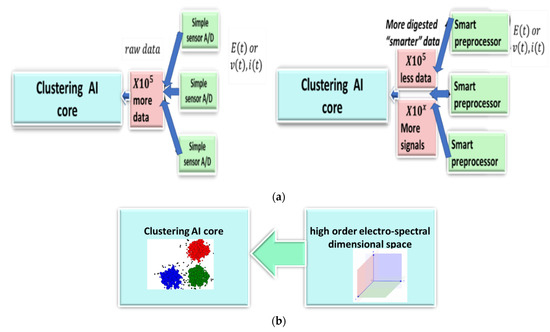
Figure 1.
(a) Classical electricity NILM architecture (left) vs. proposed “AI” NILM (right). Instead of raw data, a preprocessing module is generated to separate the “individual device” signature as much as possible. (b) Suggested architecture of high-order dimensional space feature generation module preprocessor cascaded to the clustering AI core.
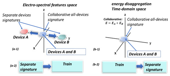
Figure 2.
(a-1) High order electro-spectral dimensional space if each axis is informative (orthogonal) and is potentially splitting the separated signatures of devices A, B from the collaborative signature (A and B) at “the origin of axes” prior to the clustering/classifier AI module operation. (a-2) The proposed algorithm initially separates the signatures of devices A, B in electro-spectral space and then trains them. Classical NILM algorithms usually work in the time-domain: (b-1) They observe “collaborative” device (A and B) signatures. (b-2) They initially train them and then learn to disaggregate the devices.
Referring to Section 2.1 terminology and definitions and observing Figure 2, a “collaborative device cluster signature” is shown in Figure 2(b-1) and is represented as the blue cluster. That signature is in time space. In high-order dimensional space, the same signature cluster is again the blue cluster. A “separated device” “signature cluster” of devices is presented in Figure 2(a-1) as red and green clusters—indicating the signature location when devices are active. There is a very distinct difference between scenario and signature. A scenario is a binary combination of active/inactive devices. A collaborative signature is this scenario signature. Additionally, in some algorithm architectures, mainly “spectral in the broad sense”, it is possible to also separate the signatures in high-order dimensional space features. For this kind of architecture, during the training stage, the signatures are already separated. For such architectures, the training is conducted over the separated device signatures, as shown in Figure 2(a-2). It is also possible to separate them, meaning that the signature is disaggregated in time space, which is for most NILM or disaggregation algorithms. Their only training periods is conducted using collaborative signatures, as shown in Figure 2(b-2), because for the time-space algorithms, the signature is not disaggregated during the training stage. It is currently unknown whether low-sampling rate algorithms, such as those that occur once every fifteen minutes, may be of high-order dimensional space. Further on, it will be possible to show that each proposed axis contributes additional information; therefore, the axes are not parallel (Section 2.7). The issue in the current paper is to generate new information that indicates that the distance between the individual electrical devices will potentially increase in a high order dimensional space. There may still be “a glue” for collaborated signature “stretching” between the device signatures, but by coloring it, it has the potential of becoming an individual device signature for the larger part of the total separate device signature. Hence, low-sampling rate algorithms operate in time-domain and the disaggregation is performed in the AI core, which performs the learning process. Therefore, most of the algorithms learn the collaborative “cluster of devices” signature. The emphasis herein is that disaggregation precedes learning. Therefore, learning will comprise of more of the separated device signatures. In the order of operation, that difference generates the reduction of mix-up probability between every two electrical devices, as will be shown later. Therefore, if this line of thought is proven for the proposed algorithm, then it will be able to obtain all of the by-product benefits mentioned in the Introduction.
2.3. A Background on Datasets—Which Datasets Fit High-Sampling Rate Algorithms and Which Low-Sampling Rate Algorithms
There are also works on NILM training datasets that are extremely important to the functionality of all of these algorithms and that may be more important than other analytics appliances. A recent work describing this is by Renaux et al. [14], who proposed an LIT dataset. This is important because (1) it states the methodology required for low-sampling rate algorithms as a dataset, and (2) because it mentions the insufficiency and inaccuracy of algorithms after they have been trained with the dataset while operating at various premises. These premises vary from one to another; (3) the work also recognizes MATLAB Simulink (which today is known as the Simscape library) as an important tool for generating dataset recordings because it is able to easily generate various combinations of electrical devices, especially those for use for industrial premises. There is the ECO dataset that is described by Santini et al. [26]. ECO stands for “Electricity Consumption and Occupancy” and is similar to other residential datasets and is based on the recording of six households. Two highly quoted datasets are REDD [27] from Stanford and REDD [28] from MIT. It is estimated that the two datasets are the same or that they at least have a common starting point. In the MIT version, there is a “describing paper” that indicates the dataset relevancy [29]; it also includes waveform recordings, which are different from energy load profiles and require a different apparatus than the smart meter does. There is the Belkin waveform dataset [19], which is known because of an international contest held on the Kaggle dataset website in 2013, where 165 participating teams collaborated. The ECO dataset from ETH University Zurich [30] is described in a paper by Santini et al. [26]. There is a UK-DALE dataset that is commonly used by NILM low-sampling rate algorithms [31] that is called the “UK Domestic Appliance Level Electricity (UK-DALE-2017)-Disaggregated appliance/whole house power”, and reference [32] provides a paper on that dataset. Looking at industrial datasets that are much less common, two are mentioned herein: WHITED [22], “Worldwide Household and Industry Transient Energy Dataset”, is a dataset of voltage and current waveform measurements that is recorded in residential and small industries. Finally, BLOND [23], “Building-Level Office Environment Dataset”, is a dataset with waveforms collected at a characteristic office building in Germany. It is a “labeled ground truth” dataset, with fifty-three electrical devices distributed within sixteen classes of electrical devices. One of the best surveys of NILM datasets, if not the best, is paper [14] by Renaux et al. The datasets for industrial premises have high sampling rates, a factor that exemplifies the challenge. Dataset generation requires special equipment that is installed on many electric sockets in the premises and usually perform a waveform or energetic load profile of ~five apartments. The equipment measures the energy load profile or voltage and current waveforms, but it also triggers the start and end timestamp points of each electrical device operation. This equipment is expensive and belongs to a dataset. Note that a vast majority of datasets are residential, indicating equipment operation cost. There are other datasets where NILM is a highly active subject, and on the surface, everything appears to be a sample. Finally, there is a recommended open-source-code Python toolkit called NILMTK [33], and there at least three papers that describe it, one of which is Nipun et al. [34]. This toolkit is evidence of discipline maturity.
2.4. A Survey of Algorithms in Order to Comprehend How to Approach the Problem
Some NILM algorithms will be reviewed in order to comprehend the gaps that may still exists despite the multitude of work that has been conducted on this topic. The review will begin by considering low-sampling rate algorithms. There are five main preliminary algorithms that mostly operate on the energetic load profile, which can be categorized according to AI architecture: (i) Denoising autoencoders: a survey and comparative study on “denoising auto encoders (DAE) was performed by Piazza et al. [35]. A convolutional deep learning DAE model was developed by Dominguez-Gonzalez et al. [36]. A denoising autoencoder prevents the autoencoder from performing identity operation by intentionally injecting noise into it. A DAE NILM is a NILM algorithm that considers energy disaggregation to be the reduction of noise; (ii) another type of NILM is the Multi-Feature Input Space (MFS) LSTM algorithm. The “multi feature” space places the individual device signature further away from other devices. An example of work on MFS LSTM is reference [37] by Hasan Rafiq et al. Work by Levron et al. [15] applies a multi-objective approach to improve NILM performance; (iii) next is the Factorial Hidden Markov Model (FHMM) NILM algorithm. Excellent examples of this algorithm can be seen in the work performed by Spanos et al. [38] as well as in the work by Zhang et al. [39], who focused on Adaptive Power Clustering process FHMM. Hidden Markov Models excel at tracking optional energy disaggregation scenarios that are being questioned while monitoring the energy load profile. (iv) The Combinatorial Optimization algorithm (CO) is next. An example of improved work conducted on CO NILM is by Wittmann [40]. Combinatorial Optimization is one of the earliest and is actually the first NILM algorithm and is mentioned in an early paper by Hart et al. [41] and more recently in another work by Wyrsch et al. [42]. It is based on recording the aggregated energy of all combinations of N appliances. The signature trained by the AI is “the collaborative” appliance signature. Then, a comparison of the energetic signature of each and every combination scenario is performed. Though it sounds simplistic, in practice, it requires much more than a single recording per scenario because devices act differently from one location to another location. (v) Next, the CNN-based “sequence-by-sequence” (CNN S-2-S) algorithm will be reviewed. As previously mentioned, disaggregation is a sequence decoding algorithm that speculates about the first appliance and then compares it to all combinations, begins speculating about the second active appliance, and so on. Sequence-to-sequence is an architecture utilizing decoder–encoder sequence analysis. Seq-to-seq CNN uses CNN for the seq-to-seq analysis, which enables the channel parallelization and better GPU usage. The architecture itself, which can be applied generally and is not NILM specific, is innovative and was introduced in 2014. J. He et al. [43] presented a CNN(S-2-S) NILM implementation. Another recent work on CNN(S-2-S) is by Huang et al. [44]. (vi) Next are the LSTM NILM and LSTM Neural NILM algorithms. One of the most notable works on LSTM NILM is by Kelly et al. [45], but it includes also other algorithms. Papers specializing in LSTM NILM are by Ochani and Rafiq et al. [46]. LSTM is an RNN algorithm that can be applied to the sequence analysis. By “regularized”, the authors Ochani et al. mean that “data regularization” occurs. This procedure adds data to a problem so as to avoid overfitting by putting a penalty function on the optimization procedure that is executed on the electricity load profile. Between two data points, two curves may pass and may be either very curly or smooth. Smooth is the regularization. So far, this review has introduced low-sampling rate algorithms operating on a quarter-hourly energy load profile. Garcia et al. [9] conducted a review on NILM algorithms. Next, some high-sampling rate NILM algorithms will be introduced briefly. High sampling rates refer to rates that occur in the range of 400 Hz–4 kHz and comprise voltage and current waveforms and not necessarily energy. These algorithms can be enabled in real-time, but as we will show in the paper with the proposed algorithm, other significant benefits exists: (1) Electromagnetic interference spectral algorithms: Patel et al. [2] present a spectral algorithm with electric parameter computation. (2) A review of high-sampling rate algorithms appears in [9]. There are common themes among all of them, and they are either spectral or electro-spectral parameters or electric parameters. What characterizes high-sampling rate algorithms is that they tend to be in high-order dimensional space, while the low-sampling rate algorithms process the data in the time-domain. Finalizing the survey, the problem of adapting NILM algorithms to industrial premises or to an external electric grid, or to more than five electrical devices, is a challenge for research. Regarding the interest of industrial NILM, industry is the largest electricity consumer in the world. The follow list presents evidence for the technical challenges of introducing NILM into industry: (i) A review paper [1] by Li et al. specifically indicates that “the application of NILM in industrial and commercial building energy detection is still a huge challenge because of its high complexity”; (ii) another issue that demonstrates the challenge is that the steady-state timestamp is insufficient, and transient recording and NILM training are required [47]; (iii) another indication that NILM implantation into industry is a challenge is that all/most datasets for industrial premises datasets are all high-frequency sampling rate algorithms [14,22,23]; (iv) finally, indirect evidence shows that all residential datasets are a collaboration of approximately five electrical devices. The reason for the challenge is deeper than the sampling rate or the supporting evidence, as seen in (i)–(iv) mentioned above, shall be researched in this article.
2.5. Spectral Theory of Non-Intrusive Load Monitoring—A Front-End Chest of Drawers
2.5.1. Simultaneous Spectra and Slow Time Representation
The raw material is a spectra of grid frequency vs. slowly varying time waveforms. Focusing on kitchens only, according to the Belkin residential dataset, electrical appliance distribution was counted by the NILM module, as shown in Figure 3.

Figure 3.
Kitchen electrical appliance distribution in the Belkin dataset computed by the proposed algorithm.
Note that time for “none” has the second largest value. Re-experimentation with “balanced” data from relatively equal counts from all devices or balancing techniques hardly changed the results. Figure 4 shows how translating the spectra-drawn peaks to Gaussian representations with three parameters each separates the electrical device signatures. This algorithm is taken from [2].
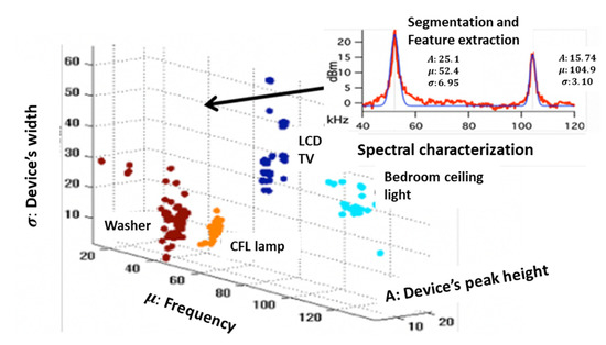
Figure 4.
Projecting the first peak of each electric device onto the three-dimensional space to obtain a single device characteristic-spectrum.
Implementation herein initially follows paper [2]. There is no open-source code for this model, and it is implemented herein and in addition to the proposed original model. The theory repeated herein is relevant for the newly proposed algorithm. After turning the voltage and current waveforms into harmonics, a spectrum is drawn. That spectrum includes baseline noise plus a new spectrum. When the recorded noise signal is subtracted from the “device+ noise” signal, the device spectrum is revealed. Noise is an alternative synonym for all of the background that is not comprehended, which stems, for example, from extra electrical devices found on the premises. There are two spectra, amplitude and phase, which are recomputed in this paper for reference. Noise is simply background spectra from the rest of the apartment.
2.5.2. Automatic Characterization of the Spectra Following Bottleneck’s Identification
Each peak in Figure 4 is characterized by three variables: (1) central frequency—distance from origin of the axis; (2) peak amplitude; and (3) width—half power height. These characteristics must be extracted automatically. If observing the Figure 4 signal as the sum of normal distributions, then we can obtain:
where:
—peak amplitude parameter, —central frequency,
—width, K–Gaussian count, and —Normal distribution.
There are two ready-made methods in Python to extract the best approximation once the desired Gaussian count is determined: the “Gaussian mixture model” (GMM) [48] and “kernel density estimation” (KDE) [49].
2.5.3. Construction of High-Order Dimensional Space
Constructing the high-order dimensional space is of dimension 3 K, where the Gaussian count may be performed arbitrarily, K = 2, or by counting up to smooth the spectra. Taking the Belkin dataset and drawing peaks for a single peak location result in the shape depicted in sub-figure in the upper right of Figure 4. Figure 3 and Figure 4 show only the kitchen electrical device turn-on count, as depicted by the proposed NILM module. As there are thirteen kitchen devices and ~64 residential devices, and in three-dimensional space, there are cluster overlaps where the proposed theory evolved in Section 3. C is justified. When there are two peaks, then two points are marked.
2.6. Proposed Theory of NILM Electro-Spectral Multidimensional Space—In Light of Insights from Separated Device Signatures vs. Collaborative Signature Theory
2.6.1. Electricity Knowledge-Based Model Construction
Three phases exist with voltage and current waveform recordings. There are N harmonics. Two of the three phases are measured. The following features are generated:
where:
—harmonics count, n—harmonic index, k—phase index;
- voltage harmonic at index n and phase k = {1,2};
current harmonic at index n and phase k = {1,2};
—reactive, active, apparent power of phase k;
K—number of phases.
Taking the N harmonics into account, one for current, K for taken phases count, and three for active, reactive, and apparent, there are dimensions:
For two phases, six harmonics—eighteen axes, are taken in the multidimensional space if two phases are sampled. The proposed algorithm goes in another direction from the method in paper [2], as there are more and different dimensions, eighteen versus three to six dimensions and electricity-spectral vs. spectral only dimensions. Not every computer can handle such big data with eighteen dimensions and comprising 20 GB of data. Connection to Part 1: all axes being spectral based causes the individual electrical device signatures farther away. After constructing an eighteen-dimensional space, in order to reduce dimensionality for the objective of visualization, a “principal component analysis” (PCA) transform is used. A tutorial on this issue can be seen in [50].
Observing previous non NILM works [51] about “multi-objective, multi-variate optimization theory”, a multi-variate design may increase design robustness [52]. In Section 2.7, it will be shown that the multi-variate increase separability of individual device signatures that may be visualized as robust, divide, and conquer. The proposed algorithm is designed according to multi-objectives, accuracy, and short training time. Designing a preprocessor that separates the signatures handles a second objective other than(1) load identification accuracy, which is the separation of individual signatures, and hat separation obtains (2) training time minimization and (3) ease of inserting new electrical devices to the training space. Thereby, the design of a high-order dimensional space may be considered as a multi-objective optimization.
2.6.2. Visualization of Eighteen-Order Dimensional-Space Spectra—Release of Bottleneck Pointed-Out by Signature Separateness
Eighteen-dimensional space is invisible to humans. The space is projected through a transformation to two-dimensional space. The proposed algorithm reduces the space order for visualization by using only principal component analysis (PCA) and linear orthogonal transformation [50]. Figure 5 shows 2D PCA of our proposed electro-spectral preprocessor over the Belkin dataset.
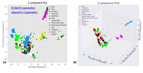
Figure 5.
PCA visualization of device spectral projection: (a) dimension reduction to 2D; (b) dimension reduction to 3D. The two-fold 2D and 3D reductions verify that even after high-order space feature construction, individual “device signatures” are often close to each other. This reinforces the role of high-order space in distancing the device signatures.
PCA by itself is not new. The usage of PCA and algorithm type characteristics to forecast qualitative algorithms and device behavior is interesting. Briefly, a linear combination of a sum of the source space dimensions reduces the order. PCA reduces the order through optimization based on the target space dimension. In PCA, destination variables are orthogonal. Figure 5 depicts what the Belkin dataset looks like in this regard. In PCA-dimensional space, the 13 electrical kitchen appliances are distinguishable. If the high-order dimensional space is imagined, similar to the state vector machine (SVM), the dimensions look like balls that have been isolated from each other, with the exception of the “None” category, which barely touches every cluster. It is important to mention that the space continues to be high-order space. PCA is only used for visualization.
Hence, five classical machine learning classification algorithms were comparatively tested after being trained on the Belkin residential spectral dataset, with the algorithms being tests on over 20% of the same portion of the Belkin dataset and cross-validated with local device waveform recordings. In the presentation of the classification methods herein, theoretical reasoning will be used to estimate whether high or low accuracy is expected and what high accuracy means when certain methods are used. PCA is an orthogonal variable and reduction representation can teach us a great deal about the accuracy of algorithms, as will be shown in the following classifier presentation.
2.6.3. Architecture Presentation
Below, an algorithm flow-diagram is presented in Figure 6. Classification is not at the core AI; it is at the virtual preprocessing model. Changing this model due to additional devices is unnecessary. The proposed 18-parameter space requires a large amount of RAM memory. Due to being spectral, the “faster than one every 15 min sampling rate” accelerates the time series, and there is wise dataset generation or enhancement. The sampling rate is faster by a factor of .

Figure 6.
NILM electric-spectral algorithm flow diagram and model-type PM 180 example sensor and the accompanying sensor reading software (same algorithm obtains identical results with SATECINC EM-720, EM-920). Research experiments all performed with PM 180.
A description of the flow diagram modules:
- (1)
- Data acquisition module: The algorithm starts with sampling voltage and current waveforms using a SatecTM PM 180 smart meter model type. At least two out of three phases are required and are sufficient. A driver to PM 180 exists on its own (“PAS” software) along with an API to the system, which is the “meter data management” system (MDM) local database. The MDM system is called “Expert power pro”.
The rest of the steps are data processing modules:
- (2)
- The time series waveforms are inserted into the FFT module to turn them into spectral signals .
- (3)
- The third module is the “electro-spectral preprocessor” that is used to cluster the AI that is illustrated in Figure 1 and implements Equation (7). This module implements the high-order dimensional space features for the AI using expert knowledge.
- (4)
- The next module is “placement of separate device signatures in features space” (4.1) takes recording segments that have been tagged by 80% of the universal dataset and translates them into points in the proposed high-order dimensional feature space. A sub-module performs 2D and 3D PCA dimensionality reduction transform to ensure that the separate device signature clusters can be visualized through human cognition. (4.2) The module then receives recordings performed by PM 180 at local residential premises, and these are currently tagged semi-automatically. In the future, they will be tagged by an automatic recording card.
- (5)
- Clustering AI core module: Ensemble learning then uses five clustering or classification cores: K-NN, decision tree, logistic classifier, ridge, and random forest. The entire toolset comprising (i) the classification report, which is most notably used for precision and recall; (ii) the AUC-ROC curve for better representation than f1-score; (iii) the confusion matrix; (iv) and the Pearson correlation heatmap. The entire toolset is operated using the high-order feature space to yield class identification.
All modules work sequentially in the order presented by Figure 6 and are implemented as a single Python software code. The code is available in [21].
2.6.4. Electric Sensor Used for Some of the Testing Dataset
The current research uses SatecINC PM 180 and EM 920 smart meters as sensory systems for waveform recording. Herein, all of the experiments were performed with the PM 180 model type. There are many other waveform recorders that are adequate for the proposed algorithm. The information is not presented for the demonstration of off-the-shelf sensors. Another powerful feature is the self-synchronization of all of the meters to a single clock using the SNTP and IRIG-B protocols.
2.6.5. K-Nearest Neighbor (KNN) in Light of PCA 2D Image and Distance Theorems
The KNN [53] algorithm usually operates after dimensionality analysis, but herein, the high-order dimension is maintained. Observing the PCA image in Figure 5 and imagining that the clusters are highly separated in terms of high-order dimensional space estimation, the nearest neighbor will yield good results. The PCA is an orthogonal axis representation, and the dimensionality reduction of the constructed multidimensional space may forecast an expectance of success of that algorithm. The number of clusters is set a priori, for example N = 13 electrical devices for the kitchen recordings. Then, distance is computed from every instance to every instance. KNN is first based on the Euclidean distance formula between instances of devices in high-order dimensional space using normalized or standardized distance. According to the number of pre-determined count of clusters, the clusters are identified using the distance formula.
2.6.6. Ridge Classifier in Light of PCA 2D Image and Distance Theorems
The ridge classifier or the Tikhonov regularization classifier [54] is a method that can be used to improve the lousy linear classifier in a problem that is usually common to multidimensional spaces. The minimization procedure is described by
where:
—is the minimization (argmin) of the loss function
—is the actual result, and —the input vector, B—the matrix that solves the minimization problem. —regularization penalty parameter. is the norm in the sense. (1) The first reason for why minimization is stuck in linear regression and in high-order dimensional space is that variables (features) are not normalized; thus, one variable may be a tiny fraction of the other or the finite accuracy of the bit representation of Equation (2). The second reason is the cost function prevents the complete zeroing of the loss that occurs when the expected value is close to the actual value, enabling training to continue. Since the problem is in multidimensional space, it is estimated that ridges will improve accuracy over linear classifiers.
2.6.7. Random Forest Classifier in Light of PCA 2D Image and Distance Theorems
The random forest classifier [55,56,57] is a non-linear algorithm that often yields extremely accurate results, experience dictates that this classifier should be successful. Figure 7 demonstrates the mode of action. The algorithm fits a different curve to each subset of points. Fitting a subset increases the accuracy of the entire algorithm. The expectation here is that this will be one of the most accurate classification algorithms.

Figure 7.
Random forest classifier algorithm graphically demonstrated. Taken from references [56,57].
The following will be discussed in the coming sections but not necessarily in the order listed here: AUC-ROC curve [58], accuracy improvement with multi-label classification [59], the effect of feature selection on the mix-up probability between two devices by the NILM algorithm [60], the effect of the signature in the feature space in previous work, such as in [61], and the entire Python classification report parameters [62].
2.6.8. Logistic Classifier in Light of PCA 2D Image and Distance Theorems
The disadvantage of the logistic classifier [55] is traditionally a linear decision boundary. If the boundary is not linear but curved, it will be less successful unless implemented differently (not implemented herein). If the clusters of different devices are distant, then the classification will be successful. If the “None” device clusters are very close to the specific devices, then it will be less successful. Thus, if successful, the algorithm will teach us about multidimensional space representation; the other factors are common knowledge. For example, the rest of the clusters originate in parts of the apartment that are outside of the kitchen. There are devices with expected signatures that are similar to kitchen devices. Observing Figure 5, PCA tells us much about expectancy from the logistic classifier, clusters of devices touching the “none” will create a large amount of confusion and will scored with the “None” category. Devices with clusters close to each other will also generate a large amount of confusion and will be scored in the “None” category. Conjecture: There is a problem regarding the ability to map a problem character based on logistic classifier performance: (a) for non-stepwise distributions, such as pseudolinear distributions (scientific term: general additive model GAM), the classic logistic classifier might yield worse accuracy than other classification algorithms, another direction of Theorem 2.7.4 Section 2.7; (b) If this scoring occurs, then the opposite is true, and it implies a curved boundary.
2.6.9. Decision Tree Classifier
The decision tree classifier is constructed such that the data are continuously split according to a certain parameter. The tree is explained by two objects: “decision nodes” and “leaves”. The leaves are the decisions or the final outcomes, and the “decision nodes” are where the data are split. A decision tree tutorial can be found in [63].
2.6.10. Scoring Methods for the Supervised Learning Algorithm
Comparative Tool #1: Computation of Classification Report: Accuracy, Precision, Recall, F-Measure and Support
For the comparative study of the algorithms, three scoring methods were used. The first method is precision computation, recall, F-measure, and support. To define the classification accuracy, one must comprehend four variables: true positives, false positives, true negatives, and false negatives. (1) Accuracy is defined graphically in Figure 8.
where:

Figure 8.
Definitions of four classification outcomes of an AI classification algorithm. (Python uses terminology classes and not objects).
—True Positive, and TN—True Negative.
FP—False Positive, and FN—False Negative.
Accuracy is the fraction of predictions that our model correctly identified. More detailed definitions are, for example, in [62]. Accuracy is the most intuitive definition that can be considered. Remember that the alternative is another candidate. The equation counts the correct positives and correct negatives over the sum of all occurrences. (2) The next classification parameter is precision:
Precision attempts to compute what proportion of positive identifications was actually correct. (3) Next is recall:
Recall attempts to compute what proportion of positive identifications was identified correctly. (4) The last parameter is f1-score:
The f1-score is the harmonic mean of precision and recall, where an F1 score reaches its best value at 1 (perfect precision and recall). Imagine parallel resistors, this is close to the equivalent resistance of parallel resistors. Finally, our classification report terminates with the micro-average, macro-average, and weighed average. The macro-average describes the average of all of the classification parameters of the same type:
where:
—parameter of instance n. Herein, electrical device —is the number of object instances; herein, the objects are the thirteen kitchen electrical devices. The “weighed average” is considered, and the number of occurrences of each instance parameter can be represented as:
where is the count of occurrences of object instance n, and the micro-average is
To observe the essence of the difference between micro and macro, the micro-average is preferable if you suspect that there might be class imbalance, as indicated in Figure 3.
Comparative Tool #2: ROC-AUC Curve
The and support are not intuitively considered as accuracy and recall. Consequently, the ROC-AUC graph and values are introduced. The ROC represents “receiver operating characteristics”, and AUC represents “area under curve”. There are many papers that provide tutorials on this subject. A clear and graphic presentation can be found in [58], further reading and a tutorial can be found in [62].
Comparative Tool #3: Confusion Matrix over the Supervised Learning Algorithms
Every column of the matrix is an object instance (electrical device) in the actual class of “electrical devices”, and every row is an object instance (electrical device) of the forecast. A matrix element is a true positives count. A matrix element is a false positive. Herein, the figure is as implemented in the Python “Scikit sklearn” library, which counts the occurrences. It could be one of the parameters.
Comparative Tool #4: Heatmap
The heatmap measures the correlation cross_val_score from the “Scikit sklearn” function and computes the Pearson coefficient formula computed with Python Numpy corrcoeff and then displays it using Seaborn lib. Correlation is multiplied herein (i.e., this paper):
where:
—the standard deviation of ;
object instance forecast;
object instance actual.
This function computes the correlation between these object instances, thereby revealing correlation in accordance with a specific classification algorithm.
2.7. A Proof That Electro-Spectral Dimensional Space Is Potentially Increasing the Separability of Individual Device Signatures
It is shown herein that the proposed electro-spectral space generated by the preprocessor potentially stretches the distance between the individual device signatures. This result is important since a combination of theoretical certainty and of experimental demonstration may convince the community to notice “collaborative” vs. “individual device” signatures as a significant performance gap. Herein, the terms orthogonal-component and additional-information are used in conjunction. If additional information exists, the cross-correlation or inner product is non-zero, and some orthogonal component of new axis exists.
Theorem 1.
Spectral harmonics of phase voltage and current harmonics contain components that are orthogonal to each other.
Proof of Theorem 1.
(1) Step 1—The result is self-explanatory for each separate phase voltage and phase current on their own, and the harmonics are orthogonal due to the fact that the Fourier basis is an orthonormal set and that it follows an inner product rule for Fourier functions:
where:
—electric phase indexed i, indicating phase index of voltage and current;
—harmonic indices;
—voltage, —current.
represent the harmonic wavefunction component of voltage/current accordingly. □
Theorem 2.
The voltage carries additional information to the current. The current can be derived from the physical definition.
Proof 1 (Formal).
where:
v—voltage;
—electric field;
—magnetic field;
—circuit length element;
—current volumetric distribution.
The first Equation (19) for the voltage waveform is a potential definition, and the second Equation (19) is the Maxwell equation, which is otherwise known as Ampere’s law, which indicates that the current surface density , which is a change of charge being the electrons flow, may be either induced from a magnetic field or from an electric field time change. However, the magnetic field is different from the electric field and is spatially orthogonal to it, and the electric field time change is different information from the electric field itself. It is a known fact that the function is at least partly linearly independent from its derivative, the Wronskian, a determinant of the function, and that its time derivative is different than zero. □
Proof 2 (Intuitive).
The voltage is the incoming wave from the grid. The current is the out-going wave from the grid and reflects interaction with the load and with the load characteristics, which are an independent transfer function.
Therefore, the spectral current contains additional information over the voltage, and feature space has a non-zero orthogonal component. For example, there are new harmonics that are generated by a harmonic generating load (HGL). □
Theorem 3.
Active and reactive power are orthogonal; they carry different information.
Proof.
where:
The following rules should be followed and are the rules of orthogonality as per active, reactive power definitions.
P—active power;
Q—reactive power, S—apparent power. □
Theorem 4.
Power is additional information to voltage and current.
Proof.
where:
The periodic averaged theory is below:
—voltage harmonic vector;
—current harmonic vector.
Apparent power is orthogonal to voltage and current and to active and reactive power. which are shown to be orthogonal from Section 2.6.3. □
Theorem 5.
The electro-spectral space proposed by this paper potentially stretches the distance between the separate “electrical device” signatures.
Proof.
where:
Since all axes in the high order electro-spectral space are orthogonal or are linearly independent, any change in any axis between two devices stretches the distance between any two electrical device signatures and separates them.
—vectors representing the signature of two electrical devices, which was initially due to lack of disaggregating information, are in the same virtual space location. □
Theorem 6.
The time domain signature at the input to the classification core is by nature non-separable and is a collaborative signature. The training that takes place is therefore for the collaborative signature.
Proof.
Let the time domain energy load profile time-series be an aggregation of two devices:
where:
electrical device 1, and electrical device 2.
There is only one Equation (23), and there are two variables. Any combination of is optional. In order to disaggregate the energy, the algorithms need to be in operation. The signature that they visualize at the entry to the clustering/classification core is collaborative, as indicated by Equation (23). During the training stage, the training is performed over the collaborative signature. Although the final result is disaggregation, the required number of training scenarios is , and the mix-up probability between electrical devices pairs is high. An example of the formulation for Equation (23) is given in [59]. □
2.8. Theoretical Computation of the Effect of Distance between Electric Device Signatures over Mix-Up Probability between Electrical Devices
The objective of this section is to prove that the mix-up probability between two devices, devices A and B, declines when the distance between the device (classes) signature clusters increases in the features space. In Section 2.7, it was proven that by using vector algebra and electricity theory, the added features increase the distance. The theoretical demonstration of the effect of distance between electrical device signatures in high-order dimensional space and the mix-up probability between device cluster A and another device, device B, as well as with all of the devices, is not included due to volume, but it is provided in a separate appendix [60]. Computational complexity is non-existent, and there is only a theorem proof. That correlation is fully obtained and constitutes the second computation enabled in the feature space. The first was Section 2.7. In short, the result is “assuming a homogeneous and isotropic distribution of ” in a normalized high-order dimensional space. This was only performed in order to simplify the computation and may be obtained using normalization technologies. Nevertheless, such technologies exist in deep learning architectures such as CNN and LSTM. Figure 9 demonstrates the feature space in previous works in order to show that “feature space” and the results herein are relevant to other works, including CNN with self-generated or semi-supervised generated features. Feature space exists even though it is not explicitly presented in most works. Hence, for distribution of “a separate device cluster of signatures” of , the Pearson correlation heatmap and mix-up probability is thus The mix-up probability (1) is also “feature space” localized—feature space does not have to be uniform in more general cases, (2) and more importantly it “declines with increasing distance between devices” in the “feature space”, a proof that was one of this paper’s objectives. Herein, distribution is assumed to be homogeneous and isotropic for computation simplification and for order of magnitude computation.
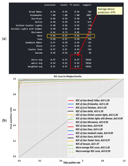
Figure 9.
KNN (a) classification report and (b) AUC-ROC curves for each of the 13 electrical devices.
Using vector algebra and electrical knowledge in Section 2.7 and then the distribution herein, the result is valid for any clustering algorithm, such as in the example of electricity theft detection shown below. Even if the clusters form a shape, referred to herein as theft/non-theft, the shapes are not homogeneous-isotropic, so the clusters are localized in space, and that is the essence of the proof. Work [64] by Wang et al. and work [65] by Wu et al., are “t-distributed stochastic neighbor embedding” (T-SNE) graphs, which are an alternative to the PCA graphs—worth observing as good examples of classes signatures, which depicted “dimensionality reduction”. In fact, there are more signatures that have been depicted in previous works, seven of which were sampled by this group, after which we stopped sampling. Being localized resulted in an infinitely spread cluster distribution declining to zero, with distance from the cluster center. If we consider the fact that the features are perhaps occasionally ignored, then they have a very important role behind the scenes.
3. Results
3.1. Comparative Study of the Algorithms
3.1.1. Specific Test Equipment Used and Project Software Language
The sensor used in this work is a “Satec PM 180” from “Satec Inc.” smart meter, that is able to provide a 4-kHz 8 channel recording. Meters collecting data for local complementary dataset recording at several residentials around Tel-Aviv. The preliminary dataset is Belkin. Identical results could be obtained with SATECINC EM 720, EM 920 model types. Application is not limited to any off-the-shelf sampling cards or devices. Local residential recordings verify non over-fitting by training using a single dataset. The reports are intentionally drawn as being suitable for deep learning object identification. Each classifier has a “thermal signature” of the entire cluster of devices. This is another conclusion from the current paper. An advantage of using non-deep-learning classifiers is that they require a much smaller training dataset but are not less accurate. Non-linear classifiers that are “non-deep-learning” are accurate. It is shown that by not using a preprocessor, the classification core learns the collaborative signature, and herein, it learns the separate device signatures. By following the accuracy figures, the visual view of the heatmap/confusion matrix is highly correlated to its accuracy report, and this is something that should be noticed. The entire code was implemented in Python and is available for download and execution in [21].
3.1.2. Classifier 1: KNN Classification Algorithm
Classification report results were trained using over 80% of the Belkin residential dataset and are shown in Figure 9a. The algorithm was tested using over 20% of the dataset and was cross-validated over live recordings using a SatecTM model type PM 180 smart meter with waveform recording. KNN was performed with 13 splits so as to match the 13 devices. Notice that “None” is the 2nd most commonly recorded device. Note that the stove and microwave have a low recall and f1-score. The higher result seen for Micro-avg is 97% and is due to the microwave and stove effect being reduced. The KNN confusion matrix yielded in Figure 9 is the strongest count, coinciding with the classification report, and 97% is classified. The AUC-ROC curves in Figure 9b are the closest to being perfect, indicating that the KNN classifier excels in this NILM. Figure 9a was computed in accordance with the “classification report” metrics developed in Section 2.6.10 as “comparative tool #1”, Equations (10)–(16). With a correctly and weighed average of {f1-score, precision, recall}, the yield of KNN works well with a large dataset. The size of the Belkin dataset is 20 GB. (2 + 3). The ROC-AUC is computed as presented at Section 2.6.10 as “comparative tool #2”. The “None” category is the most confusing, which makes sense, since “None” is “the rest of the house” and includes devices that may be similar to those on the list. An additional minor observation (4) is that the microwave and dishwasher are confusing to a minor extent. The “None” order of magnitude with each device is similar, although distribution nonuniformity is shown in Figure 3. The confusion matrix is given in Figure 10, and the correlation heatmap is displayed in Figure 10b. The color change is only due to the higher occurrence count of some devices and thus is not an indication of phenomena. Figure 10a is computed in accordance with the “confusion matrix” metrics developed in Section 2.6.10 as “comparative tool #3”.
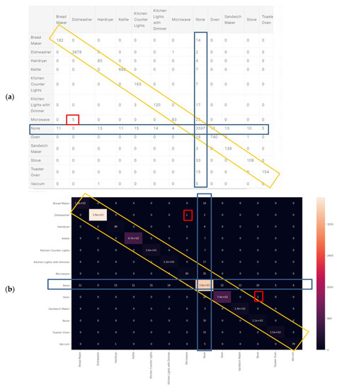
Figure 10.
KNN (a) confusion matrix and (b) Pearson’s correlation heatmap.
Figure 10b was computed in accordance with “correlation heatmap” metrics developed in Section 2.6.10, Equation (17) as “comparative tool #4”. The graphs are similar but have different confusion locations. As per Section 2.8 and external appendix [60], computation showed that the farther apart the device pairs are in the feature space, the smaller the mix-up probability is between the device pairs. There is no computational complexity, only a theorem proof. The results reflected in Figure 9 and Figure 10 are in accordance with the KNN being a non-linear classifier and were accurately recorded according to PCA Figure 5 and to the theorems in Section 2.6.2.
3.1.3. Classifier 2: Ridge Classifier
Ridge is a regularization technique that can be used to avoid overfitting. It reduces overfitting by using a penalized minimization loss function, which the reason why it is unique. Figure 11 shows a heuristic ridge classifier vs. an overfit classifier. The classification report is shown in Figure 12a. The micro-average and weighed average of {f1-score, precision, recall} are 98% accurate, and the weighted average of {f1-score, precision, recall} is 98% accurate. Figure 12a was computed in accordance with the “classification report” metrics developed in Section 2.6.10, Equations (10)–(16) and presented as “comparative tool #1”. In Figure 12b, the AUC-ROC curves are not perfect enough to create a ninety degrees corner, which indicates that for this NILM, the KNN classifier has FP and FN errors for “None” for all of the devices as well as the dishwasher, for example. “None” is the occurrence that is nearly the first distributed since the recording includes plenty of “kitchen off” time. One should be reminded that the AUC-ROC is computed according to its definition in Section 2.6.10 and presented as “comparative tool #2”. Figure 13 shows the ridge classifier confusion matrix and Pearson’s correlation heatmap. In Section 2.8 and in the external appendix [60], a computation showed that the farther apart the device pairs are in the feature space, the smaller the mix-up probability is between the device pairs. In addition to the information provided by the classification report in terms of specific algorithm performance, the only comparative information appears to be the scoring of the same parameter over all classifications.
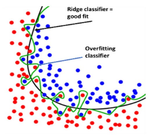
Figure 11.
Heuristic view of ridge classifier vs. an overfitting classifier. The diagram fits any none-over-fit classifier.


Figure 12.
Ridge (a) classification report and (b) AUC-ROC curves for each of the 13 electrical devices.
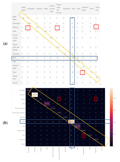
Figure 13.
Ridge classifier (a) confusion matrix and (b) correlation heatmap.
The hair-drier accuracy is reduced, which could possibly be due to it being one highly embedded sub-cluster from several hairdryer sub-clusters that are highly embedded within other device clusters. Figure 13a is the ridge algorithm confusion matrix, and Figure 13b is the ridge correlation heatmap. Figure 14b was computed in accordance with the “confusion matrix” metrics developed in Section 2.6.10 and presented as “comparative tool #3”. Figure 13b was computed in accordance with the “correlation heatmap” metrics developed in Section 2.6.10. Equation (17) and presented as “comparative tool #4”. The conclusions regarding the ridge confusion matrix (Figure 13a) and correlation heat map (Figure 13b) are similar to those of the KNN. The ridge classifier is slightly “dirtier” than KNN in terms of the correlations and confusion matrix. The results reflected by Figure 13, Figure 14 and Figure 15 are in accordance with the ridge being a non-linear correction to a linear classifier and were accurately predicted according to PCA, Figure 5, and the theorems in Section 2.6.2. The ridge classifier results are quite accurate, yet they include non-diagonal matrix elements in the confusion matrix and in the correlation heatmap and they are implemented as presented at Section 2.6.10 “comparative tool #3” and “comparative tool #4”. The AUC-ROC curves show deviation from exact precision, and they’re implemented as presented at Section 2.6.10 “comparative tool #2”. These results coincide with what is known about the ridge classifier.

Figure 14.
Random forest classifier (a) classification report and (b) AUC-ROC curves for each of the 13 electrical devices.
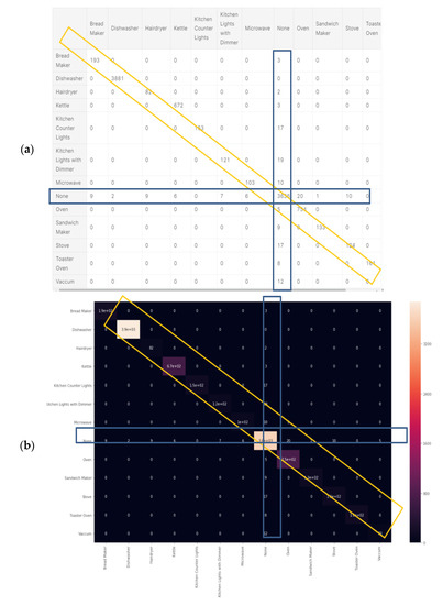
Figure 15.
Random forest classifier (a) confusion matrix and (b) Pearson’s correlation heatmap.
3.1.4. Classifier 3: Random Forest Classification
Figure 15a shows the classification report of the random forest classifier. Computation is presented at Section 2.6.10 and “comparative tool #1”. Figure 14b is computed in accordance with the “classification report” metrics developed in Section 2.5.1, Equations (10)–(16). The AUC-ROC curve in Figure 14b is close perfect, as it nearly creates a 90-degree corner, which indicates that this is very accurate on the RF classifier. AUC-ROC is presented at Section 2.6.10, as “comparative tool #2. Figure 15a shows the confusion matrix, and Figure 15b shows the correlation heatmap. Recall that in Section 2.8 and in external appendix [60], a computation showed that the farther apart the device pairs are in the feature space, the smaller the mix-up probability is between the device pairs.
There are differences from the KNN and Ridge. Relatively less accurately classified devices such as hairdryers and microwaves are in each subset. As a result, the macro-averages for precision and recall are accurately correlated using random forest classification and adapting a curve for f1-score is higher than that of the KNN and ridge. Correspondingly, the confusion matrix is cleaner, and there are no elements except for the diagonal and null row/column. Figure 15a was computed in accordance with the “confusion matrix” metrics developed in Section 2.6.10 and presented as “comparative tool #3”. Figure 15b was computed in accordance with the “correlation heatmap” metrics developed in Section 2.6.10, Equation (17) and presented as “comparative tool #4”. The results reflected by Figure 14 and Figure 15 are in accordance with random forest being a non-linear classifier and were accurately predicted according to PCA Figure 5, and PCA Section 2.6.2, and the theorems in Section 2.7.
3.1.5. Classifier 4: Decision tree classifier
Figure 16a was computed in accordance with the “classification report” metrics developed in Section 2.6.10, Equations (10)–(16) and presented as “comparative tool #1”. The AUC-ROC curves (Figure 16b) are far from being perfect and are far from being a 90 degrees corner, which indicates that the DT classifier has considerable TN and FP errors. AUC-ROC curve is presented at Section 2.6.10 as “comparative tool #2”. Figure 17a as computed in accordance with the “confusion matrix” metrics developed in Section 2.6.10 and presented as “comparative tool #3”. Figure 17b was computed in accordance with the “correlation heatmap” metrics developed in Section 2.6.10, Equation (17) and presented as “comparative tool #4”. This classifier is similar in nature to the random forest classifier because they are trees. Observing Figure 16 and Figure 17, the accuracy is seen to be slightly reduced compared to the accuracy of random forest. The confusion matrix and correlation heatmap reaffirm this result.
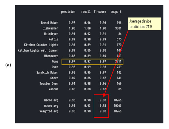
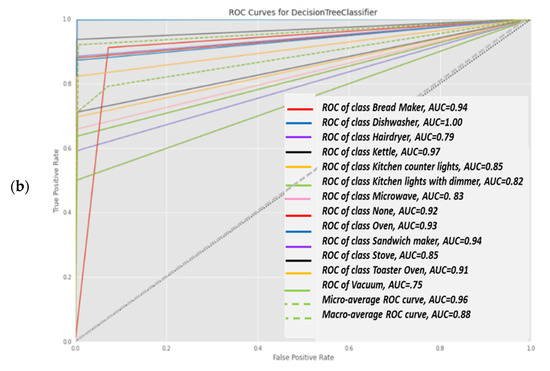
Figure 16.
Decision tree classifier (a) classification report and (b) ROC-AUC curve.
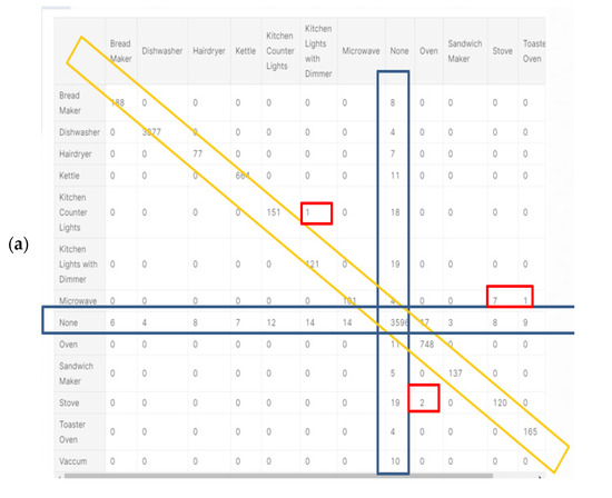
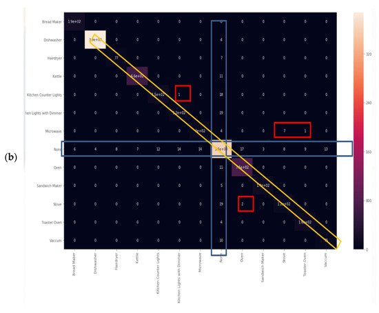
Figure 17.
Decision tree (a) confusion matrix and (b) Pearson’s correlation heatmap.
Recall that in Section 2.8 and in the external appendix [61], a computation showed that the farther apart the device pairs are in the feature space, the smaller is the mix-up probability between the device pairs is. The results, as reflected by Figure 16 and Figure 17, are in accordance with the decision tree being a non-linear classifier and were less accurately predicted according to PCA Figure 5, PCA Section 2.6.2 and the theorems in Section 2.7. All of the non-linear classifiers behave more or less accurately. The linear classifier is less accurate.
3.1.6. Classifier 5: Logistic Classifier
This classifier showed poor results, showing ~74% accuracy and plenty of confusion matrix and correlation heatmap non-diagonal elements, and the graphs are not shown herein. This is in accordance with the conjecture in Section 2.6.8 and with theorem 2.7.4 in Section 2.7.
3.2. Comparative Algorithms Results Based on References and Results, and Experiment of Training Required Scenarios Count
S comparative study between the proposed algorithm and other NILM algorithms and a comparative summary of the findings of operation of the proposed preprocessor with various clustering algorithms were described herein. Recall that the appendix in Section 2.8 proved that the mix-up probability between device pairs reduced with increasing distance. The vector algebra theorems in Section 2.7 demonstrated that the proposed features increased the distance between separate device signatures clusters.
Table 1 demonstrates a comparative study between the proposed algorithm and low-sampling rate NILMs. For the proposed algorithm, the sensory points are more expensive than conventional smart meters. With the ability to record waveforms, they are intended for another market segment with ~10 times fewer end points than residential premises. In terms of where the authors are located, they do not exist in residential premises; however, they do exist nationally in industrial premises and on the electrical grid. Therefore, although expensive, no additional hardware procurement investment is required. Table one presents an overall summary of the performance results. For the other algorithms, the figures are taken from [4,59,62].

Table 1.
Empirical accuracy and quality comparative table. Metric data taken from references [4,59,62] and the current research in this paper. All results were obtained using StatecTM PM 180 smart meter.
The AUC-ROC parameters and curves reveal a great deal of information in regard to their classifier algorithm performance in collaboration with an electro-spectral preprocessor. Its adaptation for comparative work is evident from the research. It is not the first or second NILM work that has used this parameter.
4. A Discussion on Future Research Implied by the Presented Research
What follows are suggestions of what our group considers to be strong recommendations that are enabled by technology that recently entered the smart meter market. These recommendations enable price reductions for the present paper’s proposed technology and enable an application of the paper’s proposed lessons (Section 2.7 and Section 2.8) to other works—see “Part II”.
Part I: This algorithm is the same as the one proposed in the present paper but has a lower sampling rate, which is now possible because of cheap technology that is available. Following the European Union directive dir/944/2020/EU and the 2019 benchmarking EU-28 report [66], the EU has issued a decision that states that in 2nd generation national deployments, there shall be two information channels: channel 1 comprises validated data with data of a 24/30 h latency, which is how all smart metering projects in the world are implemented. Tractebel, publisher of that reference, is the energy consultant of ENGIE. ENGIE is a multi-national energy utility company to 28 EU countries and 48 countries worldwide. The second channel is non-validated near real-time data. By including smart meter manufacturers such as Kaifa and Landis & Gyr for these countries in the EU, this can be implemented using a P1 DSMR port. This port transmits voltage and current at a rate of 0.2 Hz. The research proposes a new option for a low spectral sampling rate NILM algorithm. The slowly varying current envelope can be computed from the energy and can be FFT-ed. Similar electric parameters such as active, reactive, and power factor may be computed. Alternatively, if the current and voltage are provided as time-series measured data, then the power and energy can be computed in reverse. FFT will be able to be maintained at 0.25 Hz of a period of four seconds. Figure 18 shows a port with two smart meter examples, a Kaifa model type and a Landis & Gyr model type. Part I shall present a different spectrum than grid frequency FFT to be studied by same algorithm as presented at paper.
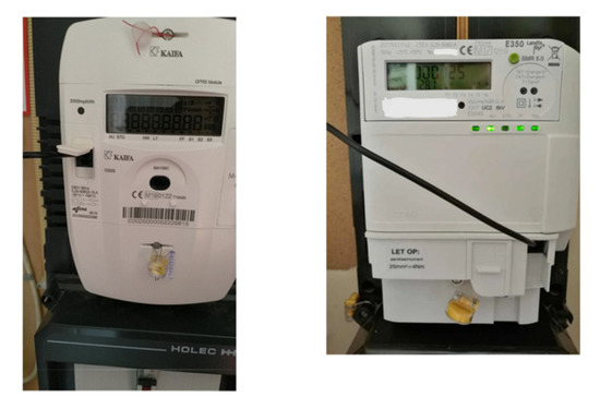
Figure 18.
P1 DSMR port enabling 0.25 Hz samples of voltage and current from smart meter. Cables are drawn from the port. The port can be connected to a transmitting modem.
Then, simply compute the harmonics over a much longer time scale:
Part II: Other works will be able to enjoy the fruits of the presented research. This algorithm functions in the same was as low-sampling rate NILM algorithms but is implemented after FFT. The other option that is recommended for future study is the known time-domain NILM algorithms that are activated after FFT and that can potentially be enhanced with a slowly varying current envelope. Ensuring that the dimensional space is spectral ensures that the separate device signatures are farther away from each other and proves that electric parameters enhance the information with regard to the cluster of devices. Therefore, the dimension count is larger, and the distance between device signatures/spatial locations are farther away.
The proposed procedure follows Equation (24). What is suggested herein is to perform the disaggregation algorithm at the spectral space over the FFT of energy or other sampled electric parameters, where the periodicity should be daily for a quarter hourly load profile and about four seconds for P1 dsmr time-series voltage and current data. The gain is that spectral data, especially when reinforced by electric knowledge based computed parameters “condensate the signature”, make it more separable to individual electrical devices. Here, the term “condensate” refers to only taking the first harmonics, and the device signature is evident. Part II spectrum is also different from grid spectrum.
- The replacement of the machine learning classifier with a CNN deep learning classifier would most probably yield a strong NILM requiring much more data. Such research, if successful, would provide evidence on points pertaining to ground zero level, electricity knowledge, and human-based knowledge of separating features, especially in terms of redirecting the self-generated features and improving their cluster of device separability.
- In this paper, the issue corresponding to the training time and the number of scenarios required for training were discussed. Model training requires a comparative study to other algorithms, and in addition, requires training using a dataset with more than 13 device types. computation of The exact order of magnitude of mix-up probability as a function of the distance between electrical devices in the features space was shown.
The FFT Part II may or may not but most likely may increase separation between the separate “device signatures”. This is a completely new area where NILM algorithms are currently not proposed, and it is a simple and straight forward research direction. It is protected under patent—see patent section.
5. Conclusions
The current research began by four objects with improvements to be made to existing NLIM algorithms. The following were listed as objects: (1) improve device identification accuracy; (2) Enhance training due to the high sampling rate; (3) create a situation where less computational effort is need in order for the algorithm to act as a gate and an enabler to industrial premises deployment; (4) report on the training process when using larger device counts than previous works; and (5) conduct a comparative study investigating several classifiers in comparison to the proposed preprocessor along with the effects and comparing these effects to previous works. Later is not a pure objective by itself, it is a requirement of proper research.
Once again, the location of entire code using for the training dataset is indicated in the Introduction, and the code is also executable there. The code is available in “free to use. The proposed algorithm was spectral and had additional electrical computation-based parameters; overall, an “eighteen parameters” “dimensional-space” was constructed. The proposed “signature theory” showed that a high-order dimensional-space of additional information at each axis is successful at the separation of the “device signatures” prior to the classification/ clustering core. In addition, that relationship was demonstrated statistically in the external appendix, which is not obvious at first sight. In terms of the algorithm itself, the cascaded classification core was implemented as an learning assemblage for five machine learning classifier algorithms: (i) KNN; (ii) ridge classifier; (iii) decision tree; (iv) random forest; and (v) logistic classifier. All of the testing was performed using a SatecINC PM 180 model smart meter with waveform recording. Identical results could also have been obtained using the EM-720 and EM-920 model types.
- (1)
- Referring to the first objective, the algorithm presented an accuracy of 98% for each and every device compared to the low-sampling rate NILM, which presented 22–92% accuracy. The accuracy at the compared low-sampling rate algorithms was device dependent at and an average of 70% was obtained. This article also compared the five performance algorithms quantitatively and showed that nonlinear classifiers are much more accurate (98%) than linear classifiers, such as the logistic classifier (75%), are. The evidence indicates that architecture selection matters and that the problem is a curly cluster shape. However, besides the implementation code and experimental testing, it was explained theoretically. It was shown that by using vector algebra and knowledge of electro-magnetic and electricity theory that the proposed features significantly increase the distance between separate device signatures in the feature space, and this was proven in the appendix, which was referred to in Section 2.8, that the mix-up probability between two devices, devices A, B, reduces with that distance. The intuition was simple. There is much less or no overlap between the signature clusters, and less overlap means less mix-up. It was shown using 2D and 3D PCA dimensionality reduction that the thirteen devices were separable, as they were colored differently. Finally, the entire Results chapter spans the quantitative study and uses standard device accuracy parameters. True positive, false positive, AUC/ROC, confusion matrix, and classification report all provide a 360° comparative view of the proposed preprocessor with various AI classifier/clustering algorithms.
- (2)
- Regarding the second objective of training time acceleration, the sampling rate of the IoT sensor is faster than low-sampling rate NILM algorithms and sensors of energetic load profile of 0.001 Hz (once every fifteen minutes). This means that training time using new devices is accelerated. There is more to acceleration than the sampling rate, but this is outside the scope of this paper and will perhaps be introduced in a future paper. Accelerated data generation is sufficient enough to explain training improvements. Observing the second and minute counts of the used Belkin dataset, it is evident that much less time is recorded compared to low-sampling rate datasets.
- (3)
- In terms of computer resources, the entire code executed a single very large dataset that included thirteen devices in no more than ten minutes over a core-i7 CPC. It required one terabyte of RAM for space construction. When considering industrial premises, there are many profile types; therefore, training time is multiplied. Training deep learning algorithms consumes time to the order of an hour per every 1000 epochs when executed on a 28 TFLOPS GPU. It was referenced in the Introduction chapter that the entry of NILM into industrial premises is a challenge.
- (4)
- Reports on training using larger devices are prevalent in previous work. It was empirically demonstrated that the algorithm is easily able to identify thirteen devices collaboratively compared to most/all previous work reporting on five devices collaboratively.
- (5)
- A comparative study was conducted using a large variety of quantitative tools, which were used over five different clustering algorithms, and the results show a large spectrum of conduct and a non-uniform behavior performance. The standard tool set included: precision, recall, AUC/ROC, confusion matrix, and Pearson correlation coefficient heatmap. The comparative study even extended beyond that to include comparison over the same parameters from previous works. The conclusion indicated more accurate results for all devices by the presented algorithm and over a larger device count.
Device identification accuracy: Here, we inspect how efficiently the proposed solution addressed the stated problem. The 2D and 3D dimensionality reduction PCA graph demonstrated that the devices signatures were separated, which was in accordance with our “signature theory”. They appear to be separated, even when observed in 2D and 3D, while actual the implementation is eighteen dimensional. The signature separation by the pre-processor prior to clustering was shown to be important the identification accuracy of each device. The order in which modules are placed is important, separation should occur first, then the modules should be trained over a cluster of electrical devices, which was the method presented herein. The alternative used by some other algorithms is training the dataset, and the training dataset learns to disaggregate the energy/devices. That order was shown to be important. An AI core, especially if operating in the time-domain, might be limited at load the disaggregation device count because effort is invested at collaborative signature disaggregation. The high accuracy that was obtained was also due to a high sampling rate, but as the paper showed, it was also due to the spectrality of the proposed algorithm vs. the time-domain of competing algorithms. This cascading architecture introduces knowledge as to how the electricity and math of how signatures are separated to improve stand-alone AI performance. The presented theoretical work showed the reduction of mix-up (confusion, correlation) probability, with stretching occurring in the distance between the electrical device clusters.
The mathematical observation that the high-order dimensional-space separates the individual device signatures from one another and that electricity knowledge increases the amount of new information on the system contribute to the distance between the device signatures in high-order dimensional space. It was shown in Section 2.7 that each of the high order dimensional space axes contribute additional information.
For future research, several research areas have been proposed that were directly inspired by the current research for benefit of other work: (ix-1) The implementation of a high-order dimensional space over a slowly varying current envelopes extracted from the energetic load profile of a smart meter. Some present-day conventional smart meters include a P1 DSMR standard unidirectional (for cyber protection) port for the communication of near real-time non-validated data (via the meter data management system) that communicate either through ZigBee, Wi-Fi, or some other form cable communication media, and the voltage and current sampled signals had rates of 0.25 Hz. This opens the gate to a new generation of NILM algorithms that are neither low-sampling rate (0.001 Hz) nor high-sampling rate (4 kHz) but are instead something in-between (0.25 Hz) and that can also act as cheap as a smart meter. That created NILMs will be very similar to the presented work, only the duration period will be different, and the spectra will be much different. Assuming that the voltage is fixed volts and that there is constant mean power during a 15 min energetic period, the current may be extracted, and a time-series of slowly varying current RMS envelope will be able to be computed. In addition, slowly varying power RMS can be computed, but it is equivalent to the current information. The slowly varying current may be FFT-ed. The period may either be daily or bi-hourly. The proposed sampling rate will be periodic according to the sampled quarter hourly period. It has been shown that such future research is interesting and beneficial and may potentially be of added value. (ix-2) Another future research direction suggested by the current research is to take one of five presented low-sampling rate algorithms and to FFT the raw data and to then perform “linguistic like” analysis on it. Alternatively, computing the slowly varying current envelope from the energy load profile and combining it as a multi-vector {energy, current} and then performing FFT over that information followed by operating linguistic like” analysis over it presents additional possibilities for future research. The high-order dimensional space preprocessor is suitable for any clustering core. This includes deep learning cores that were not studied in the current research. In conclusion the research has two main added values. One is the presented algorithm, and the other is much improved mathematical/physical comprehension of how load identification should work. The current study proposes an alternative line of NILM development. Instead of thinking about a more advanced AI, AI design should be considered in light of more profound national deployment requirements, namely by shortening the training time by having the algorithm undergo less training. This will create dramatic performance improvements to modest algorithms.
6. Patents
The algorithm is a module inside a pending patent for the electric grid deciphering system and apparatus. A patent is in the provisional registration process, and the file number is 2020119 by Ramot, the TAU proprietary commercialization company. The patent includes NILM algorithms for the range of .
Author Contributions
Conceptualization, N.C. and D.S.; methodology, N.C. and D.S; software, N.C. and M.D. All authors have read and agreed to the published version of the manuscript.
Funding
This research received not external funding.
Institutional Review Board Statement
Not applicable.
Informed Consent Statement
Not applicable.
Data Availability Statement
Belkin dataset reference [19], local dataset—on demand.
Conflicts of Interest
The authors declare no conflict of interest.
References
- Zhuang, M.; Shahidehpour, M.; Li, Z. An Overview of Non-Intrusive Load Monitoring: Approaches, Business Applications, and Challenges. In Proceedings of the 2018 International Conference on Power System Technology, POWERCON 2018—Proceedings, Guangzhou, China, 6–8 November 2018; Institute of Electrical and Electronics Engineers Inc.: Piscataway, NJ, USA, 2019; pp. 4291–4299. [Google Scholar]
- Gupta, S.; Reynolds, M.S.; Patel, S.N. ElectriSense: Single-Point Sensing Using EMI for Electrical Event Detection and Classification in the Home. In Proceedings of the 12th ACM International Conference on Ubiquitous Computing, Copenhagen, Denmark, 26–29 September 2010; pp. 139–148. [Google Scholar]
- Singer, S.; Ozeri, S.; Shmilovitz, D. A pure realization of Loss-Free Resistor. IEEE Trans. Circuits Syst. 2004, 51, 1639–1647. [Google Scholar] [CrossRef]
- Xiaohan, S.; Rafiq, H. “Non-Intrusive Load Monitoring” Scholarly Community Encyclopedia, “Zhejiang University | ZJU · Department of Mathematics, Shandong University | SDU · School of Electrical Engineering. Available online: https://encyclopedia.pub/1384 (accessed on 28 October 2020).
- Verma, A.; Anwar, A.; Mahmud, M.A.P.; Ahmed, M.; Kouzani, A. A Comprehensive Review on the NILM Algorithms for Energy Disaggregation. arXiv 2021, arXiv:2102.12578. [Google Scholar]
- Jiang, L.; Li, J.; Luo, S.; Jin, J.; West, S. Literature review of power disaggregation. In Proceedings of the 2011 International Conference on Modelling, Identification and Control, Innsbruck, Austria, 24–26 October 2011; pp. 38–42. [Google Scholar] [CrossRef]
- Hosseini, S.S.; Agbossou, K.; Kelouwani, S.; Cardenas, A. Non-intrusive load monitoring through home energy management systems: A comprehensive review. Renew. Sustain. Energy Rev. 2017, 79, 1266–1274. [Google Scholar] [CrossRef]
- Herrero, J.R.; Murciego, Á.L.; Barriuso, A.L.; de La Iglesia, D.H.; González, G.V.; Rodríguez, J.M.C.; Carreira, R. Non-intrusive load monitoring (nilm): A state of the art. In Proceedings of the International Conference on Practical Applications of Agents and Multi-Agent Systems, Porto, Portugal, 21–23 June 2017; Springer: Porto, Portugal, 2017; pp. 125–138. [Google Scholar]
- Ruano, A.; Hernandez, A.; Ureña, J.; Ruano, M.; Garcia, J. NILM Techniques for Intelligent Home Energy Management and Ambient Assisted Living: A Review. Energies 2019, 12, 2203. [Google Scholar] [CrossRef] [Green Version]
- Shin, C.; Rho, S.; Lee, H.; Rhee, W. Data requirements for applying machine learning to energy disaggregation. Energies 2019, 12, 1696. [Google Scholar] [CrossRef] [Green Version]
- Energy Disaggregation from Non-Intrusive Load Monitoring: AM207. Available online: https://www.youtube.com/watch?v=9a8dR9NEe6w (accessed on 6 May 2016).
- D’Incecco, M.; Squartini, S.; Zhong, M. Transfer Learning for Non-Intrusive Load Monitoring. IEEE Trans. Smart Grid 2020, 11, 1419–1429. [Google Scholar] [CrossRef] [Green Version]
- Delfosse, A.; Hebrail, G.; Zerroug, A. Deep Learning Applied to NILM: Is Data Augmentation Worth for Energy Disaggregation? In Proceedings of the ECAI 2020, Santiago de Compostela, Spain, 29 August–8 September 2020; Volume 325, pp. 2972–2977. [Google Scholar]
- Renaux, D.P.B.; Pottker, F.; Ancelmo, H.C.; Lazzaretti, A.E.; Lima, C.R.E.; Linhares, R.R.; Oroski, E.; Nolasco, L.; Lima, L.T.; Mulinari, B.M.; et al. A Dataset for Non-Intrusive Load Monitoring: Design and Implementation. Energies 2020, 13, 5371. [Google Scholar] [CrossRef]
- Machlev, R.; Belikov, J.; Beck, Y.; Levron, Y. MO-NILM: A multi-objective evolutionary algorithm for NILM classification. Energy Build. 2019, 199, 134–144. [Google Scholar] [CrossRef]
- Machlev, R.; Tolkachov, D.; Levron, Y.; Beck, Y. Dimension reduction for NILM classification based on principle component analysis. Electr. Power Syst. Res. 2020, 187, 134–144. [Google Scholar] [CrossRef]
- Aho, A.V.; Hopcroft, J.E.; Ullman, J.D. The Design and Analysis of Computer Algorithms; Addison Wesley: London, UK; Amsterdam, The Netherlands; Don Mills, ON, Canada; Sydney, Australia, 1974. [Google Scholar]
- Arora, S.; Barak, B. Computational Complexity: A Modern Approach; Cambridge University Press: Cambridge, UK, 2009; ISBN 978-0-521-42426-4. [Google Scholar]
- Belkin Residential Apartments Waveforms Dataset. Available online: https://www.kaggle.com/c/belkin-energy-disaggregation-competition/data (accessed on 26 February 2013).
- REDD Residential Dataset. Available online: http://redd.csail.mit.edu/ (accessed on 26 February 2019).
- Paper’s Code Location. Available online: https://www.kaggle.com/moshedo500/nilm-project (accessed on 26 February 2019).
- Kahl, M.; Haq, A.; Kriechbaumer, T.; Jacobsen, H.A. WHITED—A Worldwide Household and Industry Transient Energy Data Set. In Proceedings of the 3rd International Workshop on Non-Intrusive Load Monitoring, Vancouver, BC, Canada, 14–15 May 2016. [Google Scholar]
- Kriechbaumer, T.; Jacobsen, H.A. BLOND, a building-level office environment dataset of typical electrical appliances. Sci. Data 2018, 5, 180048. [Google Scholar] [CrossRef]
- Calamaro, N.; Beck, Y.; Ben Melech, R.; Shmilovitz, D. An Energy-Fraud Detection-System Capable of Distinguishing Frauds from Other Energy Flow Anomalies in an Urban Environment. Sustainability 2021, 13, 10696. [Google Scholar] [CrossRef]
- Singhal, V.; Maggu, J.; Majumdar, A. Simultaneous Detection of Multiple Appliances From Smart-Meter Measurements via Multi-Label Consistent Deep Dictionary Learning and Deep Transform Learning. IEEE Trans. Smart Grid 2019, 3, 2969–2978. [Google Scholar] [CrossRef] [Green Version]
- Beckel, C.; Kleiminger, W.; Cicchetti, R.; Staake, T.; Santini, S. The ECO data set and the performance of non-intrusive load monitoring algorithms. In Proceedings of the BuildSys’14: 1st ACM International Conference on Embedded Systems for Energy-Efficient Buildings, Memphis, TN, USA, 5–6 November 2014; Srivastava, M., Ed.; Association for Computing Machinery: New York, NY, USA; pp. 80–89. [Google Scholar]
- Stanford University. Residential Energy Disaggregation Data Set. Initial REDD. Available online: https://peec.stanford.edu/research/residential-energy-disaggregation-dataset-redd (accessed on 26 April 2021).
- MIT. Reference Energy Disaggregation Data Set (REDD). Available online: https://energy.duke.edu/content/reference-energy-disaggregation-data-set-redd (accessed on 26 April 2012).
- Kolter, J.Z.; Johnson, M.J. Redd: A public data set for energy disaggregation research. Artif. Intell. 2011, 25, 59–62. [Google Scholar]
- ECO Dataset. Available online: https://www.vs.inf.ethz.ch/res/show.html?what=eco-data (accessed on 26 February 2019).
- UK Domestic Appliance Level Electricity(UK-DALE-2017)-Disaggregated Appliance/Whole House Power. Available online: https://ukerc.rl.ac.uk/DC/cgi-bin/edc_search.pl/?WantComp=138 (accessed on 26 April 2017).
- Kelly, J.; Knottenbelt, W. The UK-DALE dataset, domestic appliance-level electricity demand and whole-house demand from five UK homes. Sci. Data 2015, 2, 150007. [Google Scholar] [CrossRef] [Green Version]
- NILMTK: An Open-Source-Code NILM Library. Available online: https://nilmtk.github.io/ (accessed on 26 April 2014).
- Batra, N.; Kelly, J.; Parson, O.; Dutta, H.; Knottenbelt, W.; Rogers, A.; Singh, A.; Srivastava, M. NILMTK: An open-source toolkit for non-intrusive load monitoring. In Proceedings of the 5th International Conference on Future Energy Systems, Cambridge, UK, 11–13 June 2014. [Google Scholar]
- Bonfigli, R.; Felicetti, A.; Principi, E.; Fagiani, M.; Squartini, S.; Piazza, F. Denoising autoencoders for non-intrusive load monitoring: Improvements and comparative evaluation. Energy Build. 2018, 158, 1461–1474. [Google Scholar] [CrossRef]
- García-Pérez, D.; Pérez-López, D.; Díaz-Blanco, I.; González-Muñiz, A.; Domínguez-González, M.; Vega, A.A.C. Fully-Convolutional Denoising Auto-Encoders for NILM in Large Non-Residential Buildings. IEEE Trans. Smart Grid 2021, 12, 2722–2731. [Google Scholar] [CrossRef]
- Rafiq, H.; Shi, X.; Zhang, H.; Li, H.; Ochani, M.K. A Deep Recurrent Neural Network for Non-Intrusive Load Monitoring Based on Multi-Feature Input Space and Post-Processing. Energies 2020, 13, 2195. [Google Scholar] [CrossRef]
- Jia, R.; Gao, Y.; Spanos, C.J. A fully unsupervised non-intrusive load monitoring framework. In Proceedings of the 2015 IEEE International Conference on Smart Grid Communications (SmartGridComm), Miami, FL, USA, 2–5 November 2015; pp. 872–878. [Google Scholar] [CrossRef]
- Zhao, W.; Wang, C.; Peng, W.; Liu, W.; Zhang, H. Non-intrusive load monitoring using factorial hidden markov model based on adaptive density peak clustering. Energy Build. 2021, 244, 111025. [Google Scholar] [CrossRef]
- Flores, M.J.R.; Wittmann, M.F. Optimization Applied to Residential Non-Intrusive Load Monitoring. Master’s Thesis, Universidade Estadual de Campinas, Campinas, Brazil, 2017. [Google Scholar]
- Hart, G.W. Nonintrusive appliance load monitoring. Proc. IEEE 1992, 80, 1870–1891. [Google Scholar] [CrossRef]
- Holweger, J.; Dorokhova, M.; Bloch, L.; Ballif, C.; Wyrsch, N. Unsupervised algorithm for disaggregating low-sampling-rate electricity consumption of households. Sustain. Energy Grids Netw. 2019, 19, 100244. [Google Scholar] [CrossRef] [Green Version]
- Chen, U.; Wang, Q.; He, Z.; Chen, K.; Hu, J.; He, J. Convolutional sequence to sequence non-intrusive load monitoring. J. Eng. 2018, 17, 1860–1864. [Google Scholar] [CrossRef]
- Zhou, G.; Li, Z.; Fu, M.; Feng, Y.; Wang, X.; Huang, C. Sequence-to-Sequence Load Disaggregation Using Multiscale Residual Neural Network. IEEE Trans. Instrum. Meas. 2021, 70, 1–10. [Google Scholar] [CrossRef]
- Kelly, J.; Knottenbelt, W. Neural NILM: Deep neural networks applied to energy disaggregation. In Proceedings of the ACM BuildSys, Seoul, Korea, 4–5 November 2015; pp. 55–64. [Google Scholar]
- Rafiq, H.; Zhang, H.; Li, H.; Ochani, M.K. Regularized LSTM Based Deep Learning Model: First Step towards Real-Time Non-Intrusive Load Monitoring. In Proceedings of the 2018 IEEE International Conference on Smart Energy Grid Engineering (SEGE), Oshawa, ON, Canada, 12–15 August 2018; pp. 234–239. [Google Scholar] [CrossRef]
- Lin, G.Y.; Lee, S.C.; Hsu, Y.J.; Jih, W.R. Applying Power Meters for Appliance Recognition on the Electric Panel. In Proceedings of the 5th IEEE Conference on Industrial Electronics and Applications, Melbourne, Australia, 15–17 June 2010; pp. 2254–2259. [Google Scholar]
- Reynolds, D. Gaussian Mixture Models. In Encyclopedia of Biometrics; Springer Science Business Media: New York, NY, USA, 2009; pp. 659–663. [Google Scholar]
- Zucchini, W.; Berzel, A.; Nenadic, O. Applied Smoothing Techniques. Part I: Kernel Density Estimation. 2003, pp. 5–19. Available online: https://docplayer.net/60547422-Applied-smoothing-techniques-part-1-kernel-density-estimation-walter-zucchini.html (accessed on 26 February 2017).
- Smith, L.I.A. Tutorial on Principal Components Analysis; University of Otago: Dunedin, New Zeeland, 2002; Volume 51, pp. 5–24. [Google Scholar]
- Marler, R.T.; Arora, J.S. Survey of multi-objective optimization methods for engineering. Struct. Multidiscipl. Optim. 2004, 26, 369–395. [Google Scholar] [CrossRef]
- Deb, K.; Gupta, H. Introducing robustness in multi-objective optimization. J. Evol. Comput. 2006, 14, 463–494. [Google Scholar] [CrossRef]
- Sutton, O. Introduction to k Nearest Neighbor Classification and Condensed Nearest Neighbor Data Reduction; University of Leicester: Leicester, UK, 2012. [Google Scholar]
- Oladunni, O.O.; Trafalis, T.B. A pairwise reduced kernel-based E = multi-classification Tikhonov regularization machine. In Proceedings of the International Joint Conference on Neural Networks (IJCNN’06), Vancouver, BC, Canada, 16–21 July 2006; pp. 130–137. [Google Scholar] [CrossRef]
- Available online: https://towardsdatascience.com/machine-learning-basics-random-forest-classification-499279bac51e?gi=dff15d2726cc (accessed on 26 June 2021).
- Jordan, A.Y. On discriminative versus generative classifiers: A comparison of logistic classifier and naive Bayes. Adv. Neural Inform. Process. Syst. 2001, 14, 605–610. [Google Scholar]
- Afanador, N.L.; Smolinska, A.; Tran, T.; Blanchet, L. Unsupervised random forest: A tutorial with case studies. J. Chemometr. 2016, 30, 232–241. [Google Scholar] [CrossRef]
- Understanding AUC-ROC Curve. Available online: https://towardsdatascience.com/understanding-auc-roc-curve-68b2303cc9c5 (accessed on 26 June 2018).
- Massidda, L.; Marrocu, M.; Manca, S. Non-Intrusive Load Disaggregation by Convolutional Neural Network and Multilabel Classification. Appl. Sci. 2020, 10, 1454. [Google Scholar] [CrossRef] [Green Version]
- External Appendix: File Appendix_Proof_Computational_Complexity_Post_Review1.docx. Available online: https://www.kaggle.com/moshedo500/nilm-project (accessed on 26 June 2021).
- Kim, J.; Le, T.T.H.; Kim, H. Nonintrusive load monitoring based on advanced deep learning and novel signature. Comput. Intell. Neurosci. 2017, 2017, 1–23. [Google Scholar] [CrossRef]
- Powers, D.M.W. Evaluation: From Precision, Recall and F-Measure to ROC, Informedness, Markedness & Correlation. J. Mach. Learn. Tech. 2011, 2, 37–63. [Google Scholar]
- Myles, A.J.; Feudale, R.N.; Liu, Y.; Woody, N.A.; Brown, S.D. An introduction to decision tree modeling. J. Chemometr. 2004, 18, 275–285. [Google Scholar] [CrossRef]
- Li, J.; Wang, F. Non-Technical Loss Detection in Power Grids with Statistical Profile Images Based on Semi-Supervised Learning. Sensors 2020, 20, 236. [Google Scholar] [CrossRef] [PubMed] [Green Version]
- Hu, T.; Guo, Q.; Shen, X.; Sun, H.; Wu, R.; Xi, H. Utilizing unlabeled data to detect electricity fraud in AMI: A semi-supervised deep learning approach. IEEE Trans. Neural Netw. Learn. Syst. 2019, 30, 1–13. [Google Scholar] [CrossRef] [PubMed]
- Alaton, C.; Tounquet, F.; Directorate-General for Energy; European Commission; Tractebel Impact ENGIE. Benchmarking Smart Metering Deployment in the EU-28 Final Report; European Union: Brussel, Belgium, 2020. [Google Scholar]
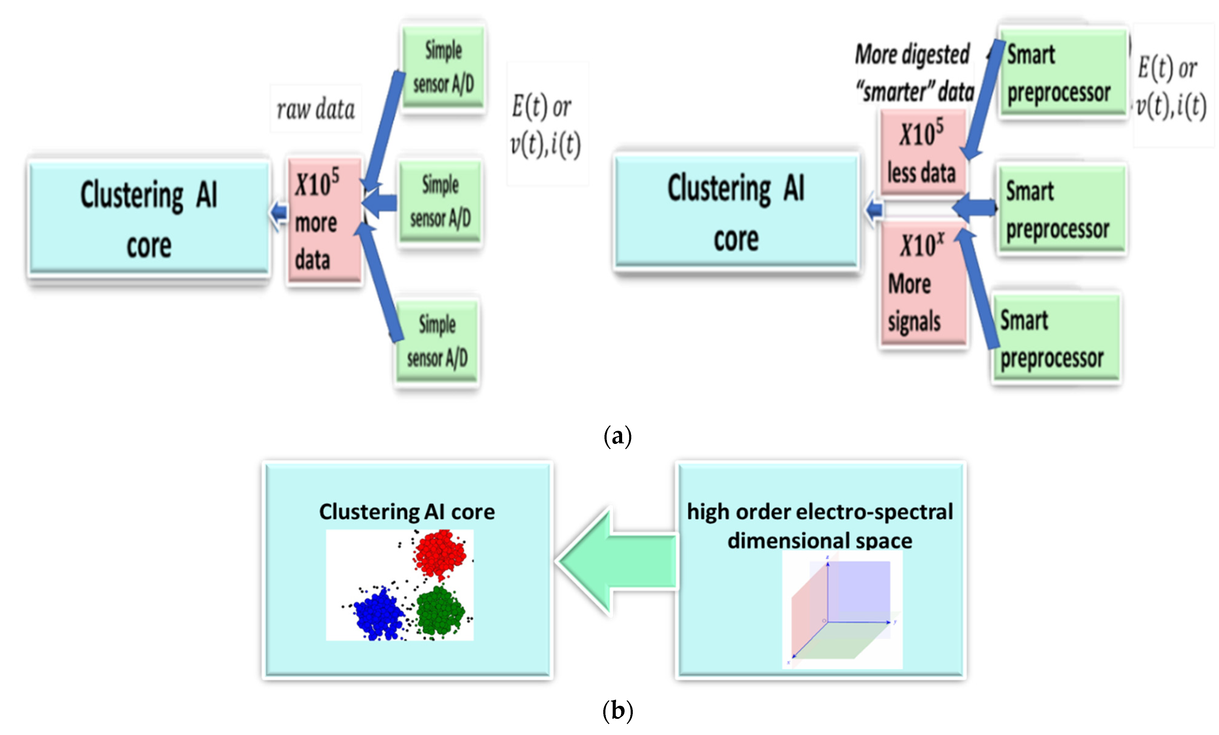
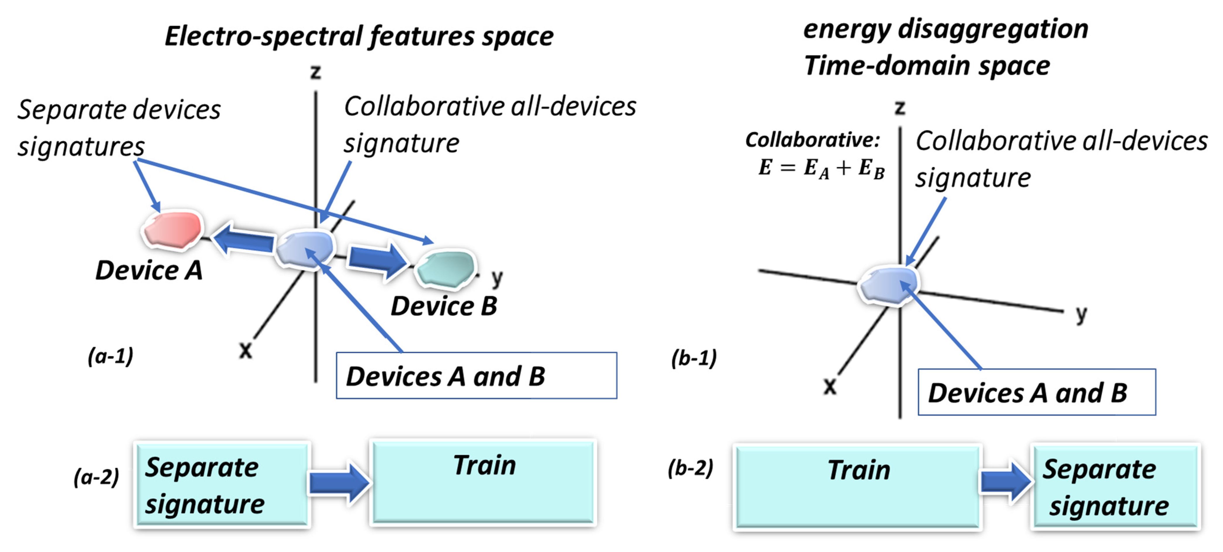
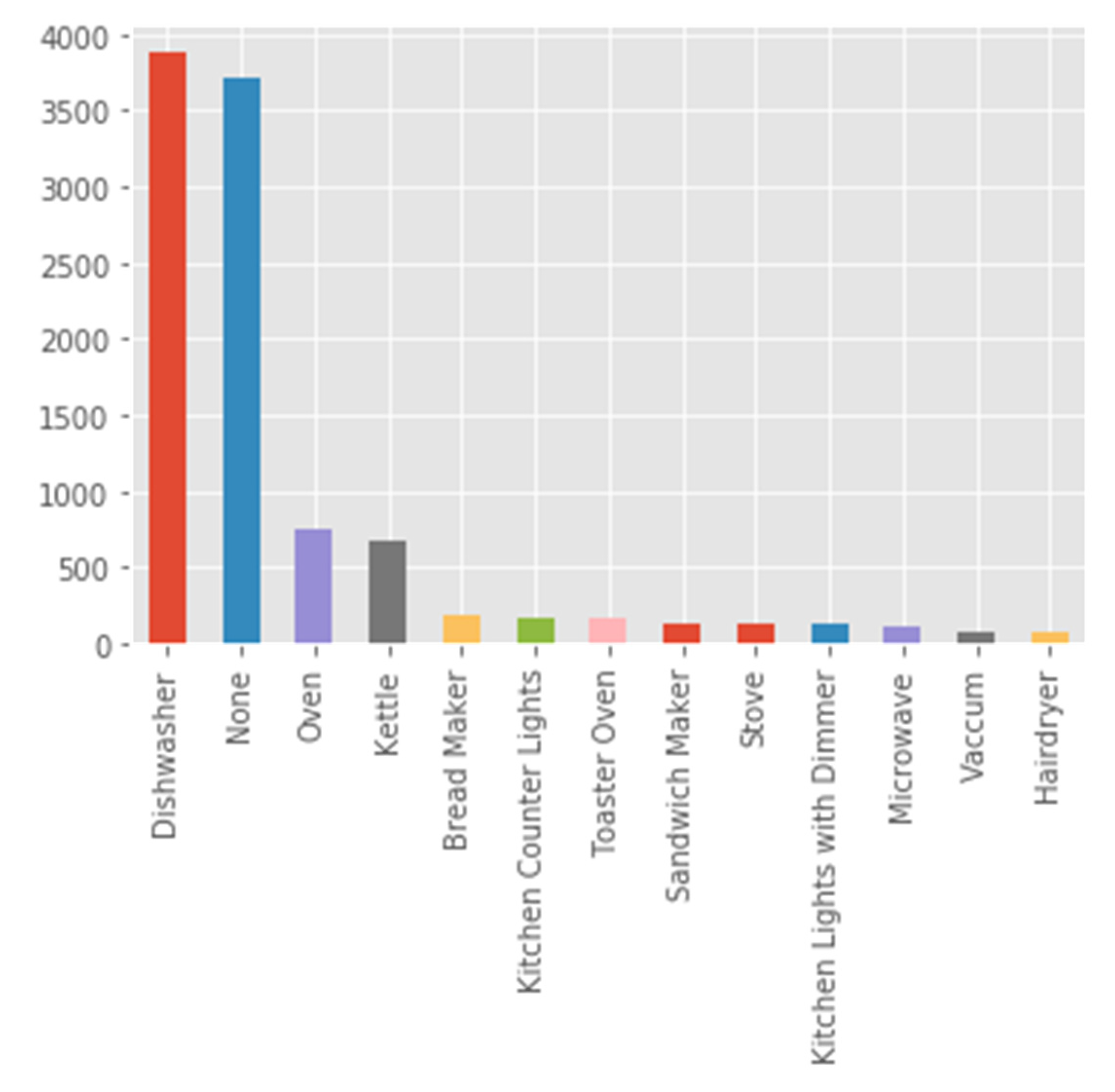
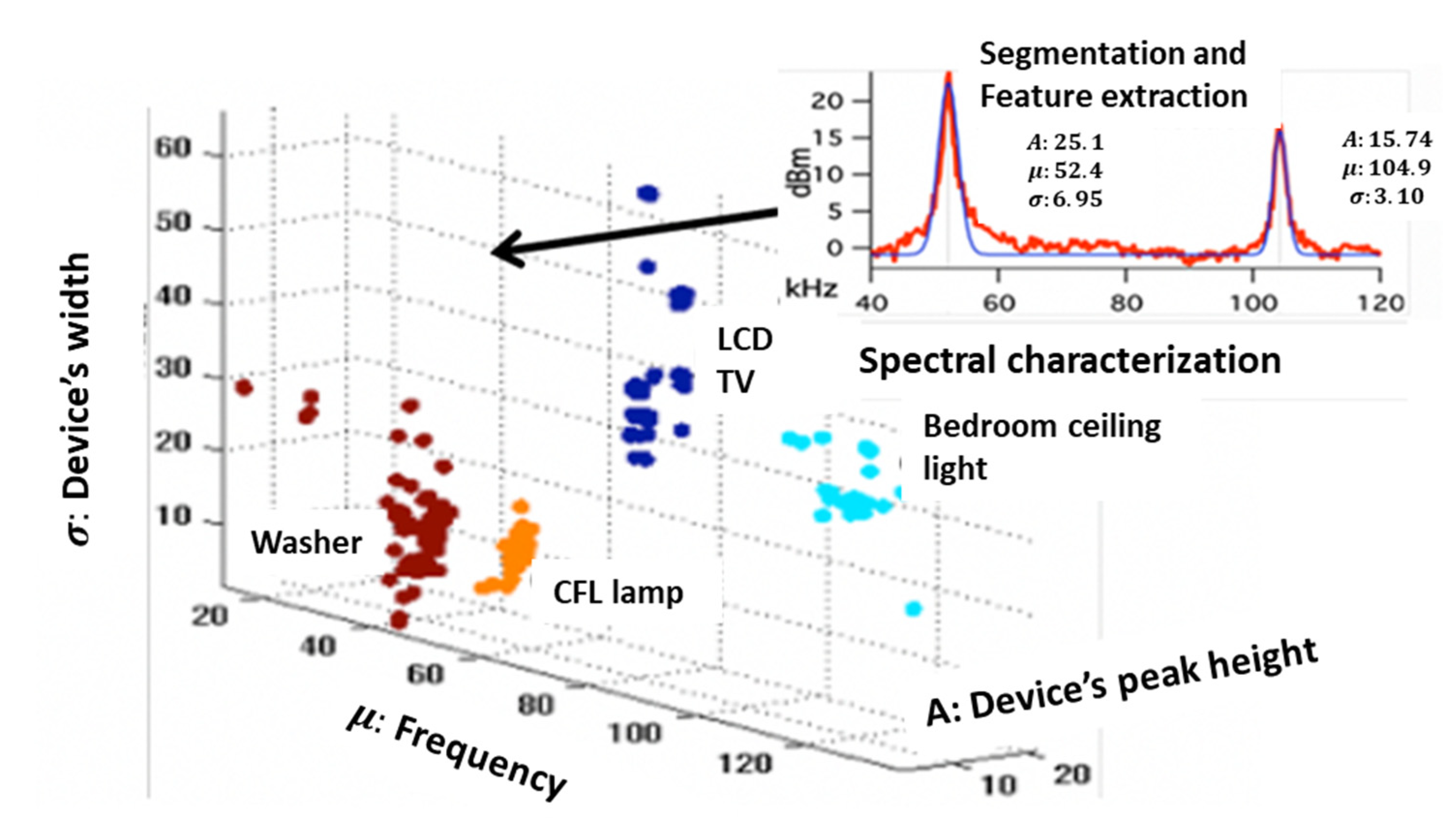
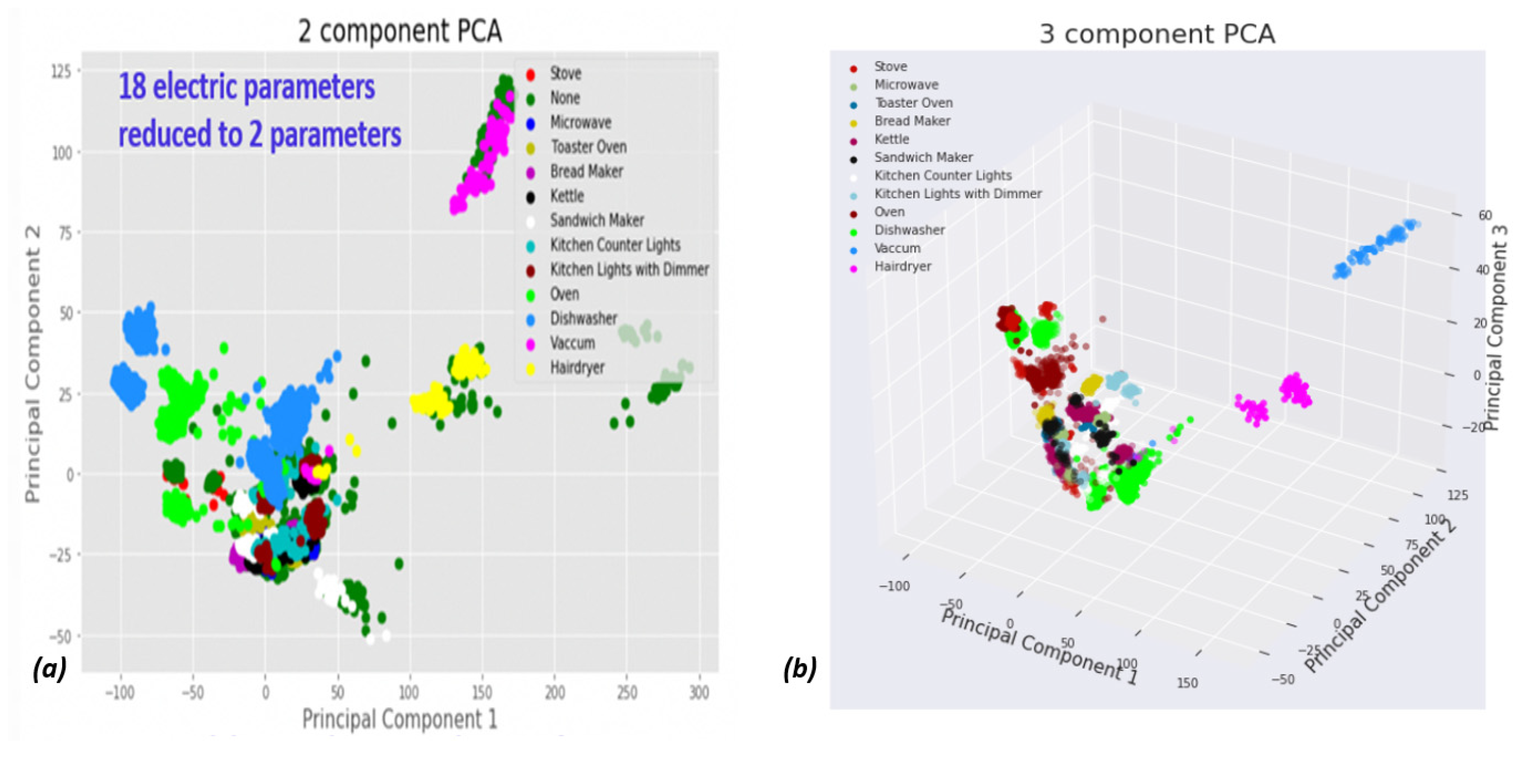
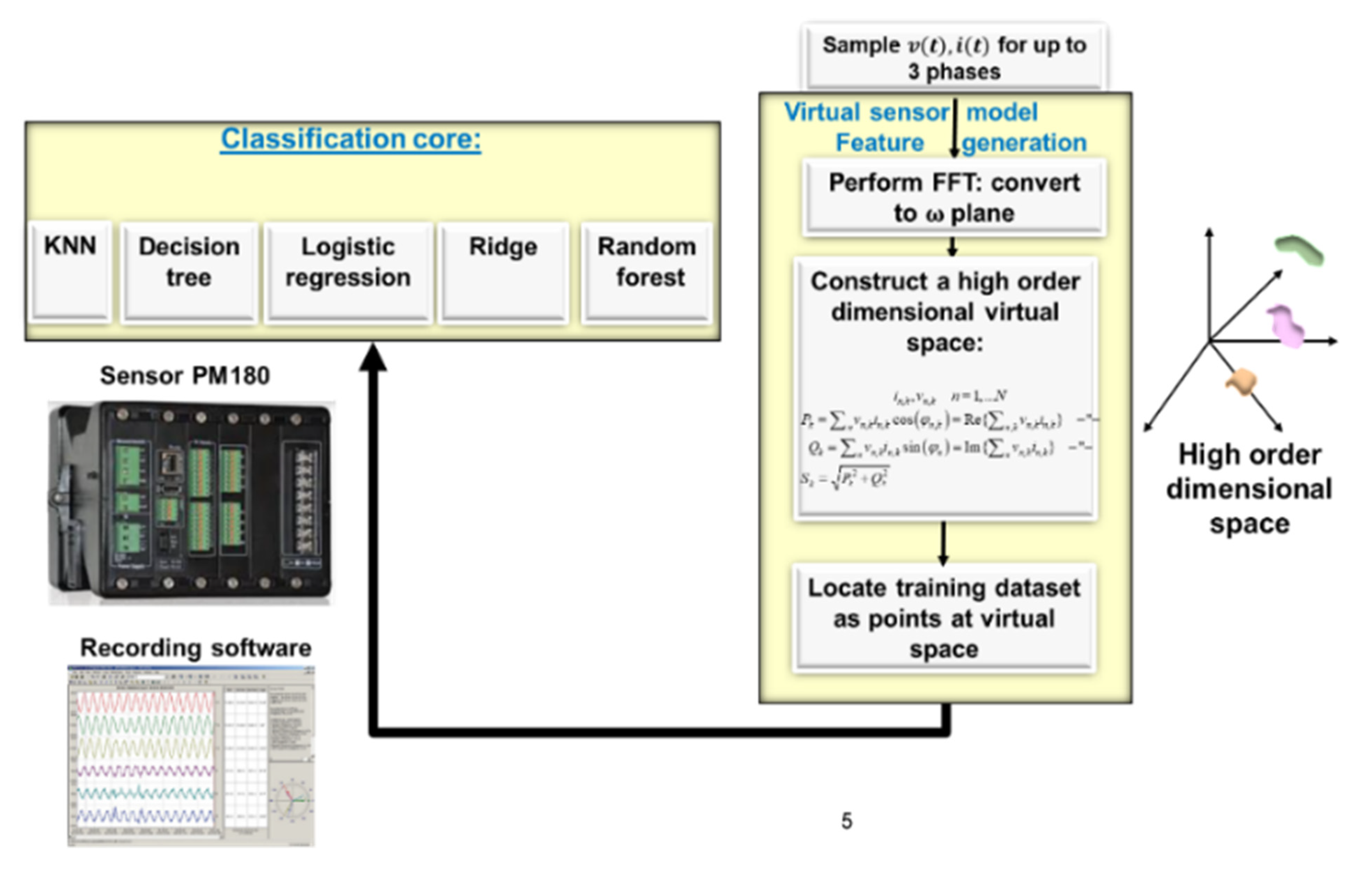
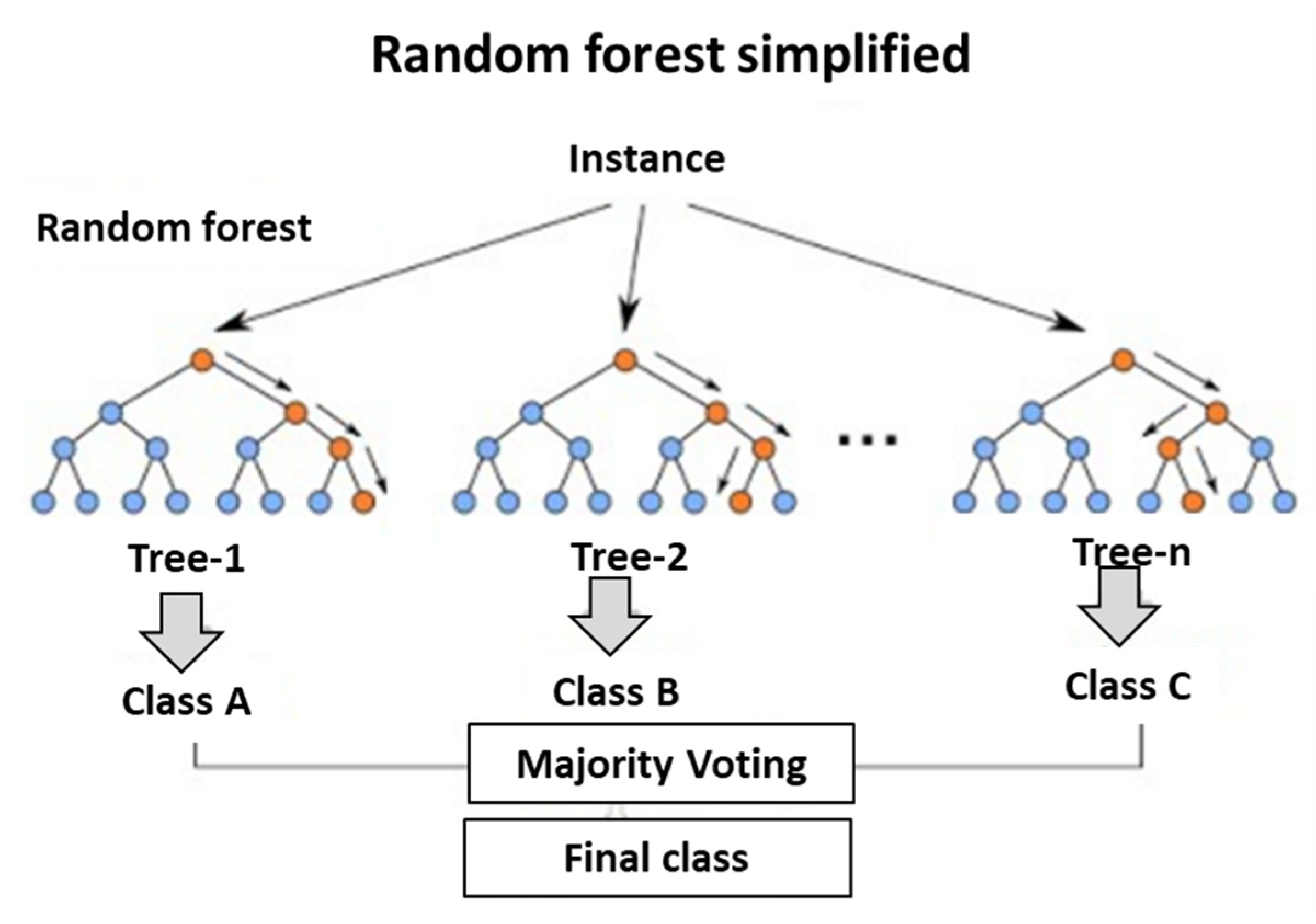
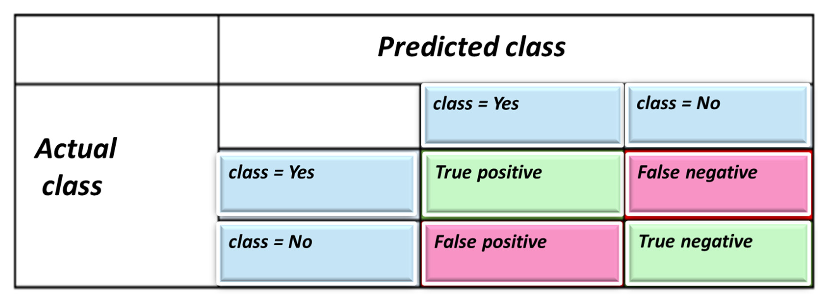
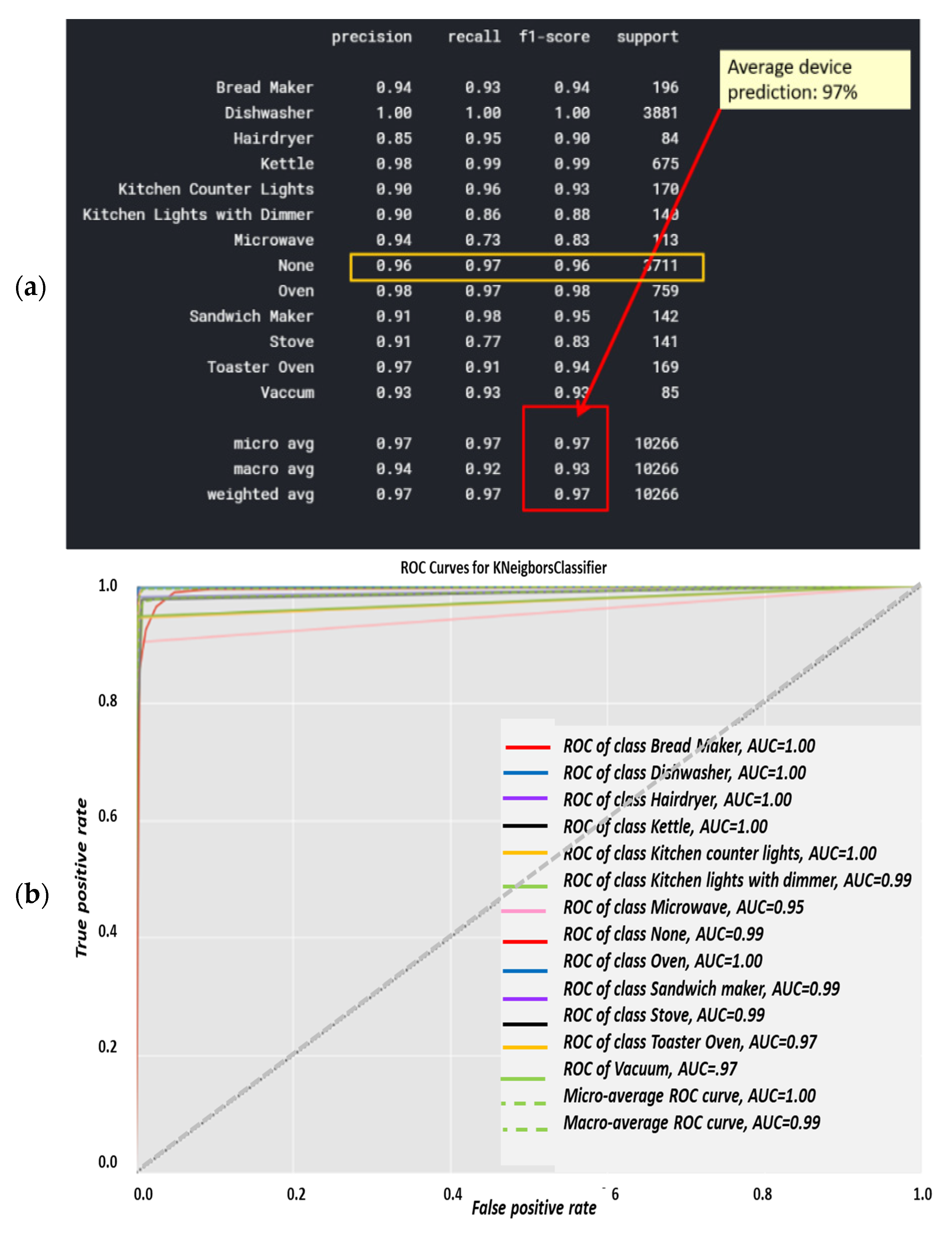


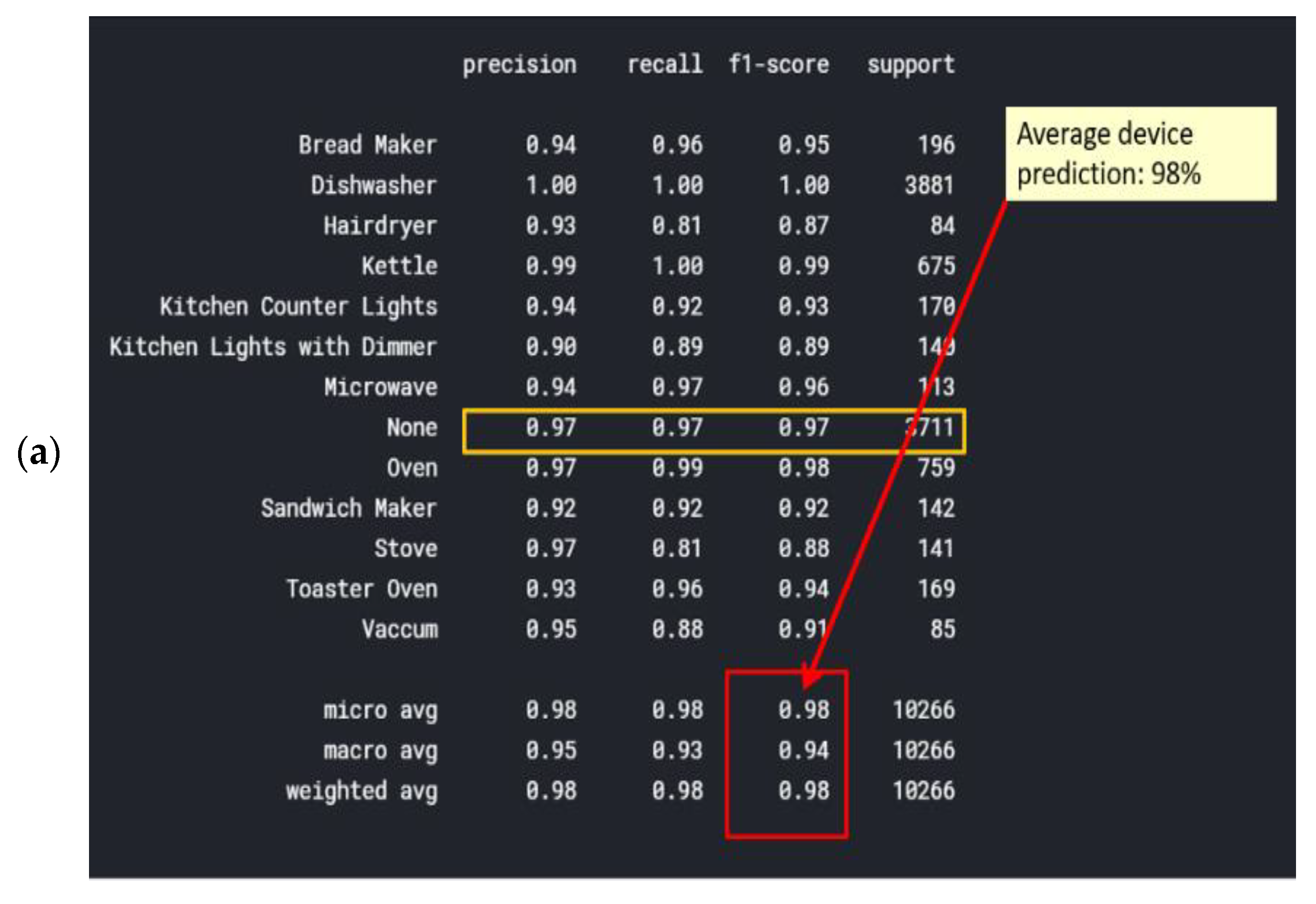
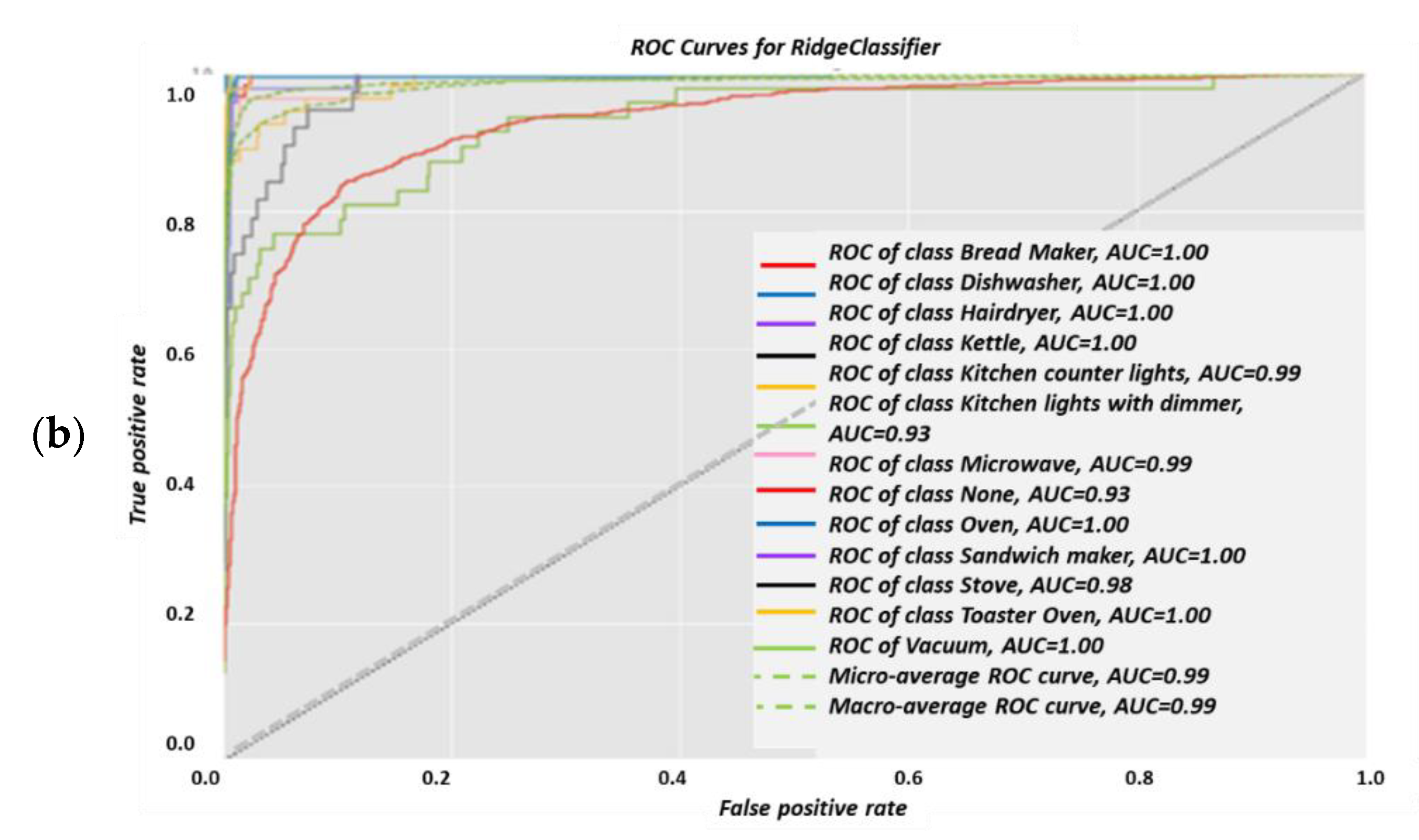

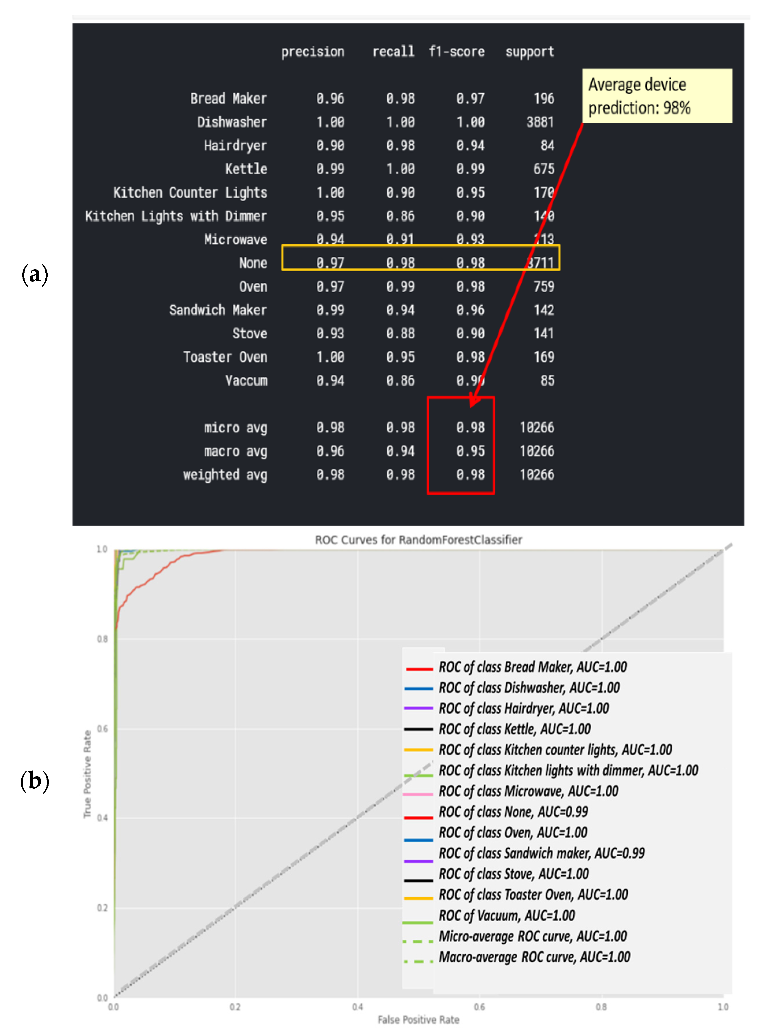
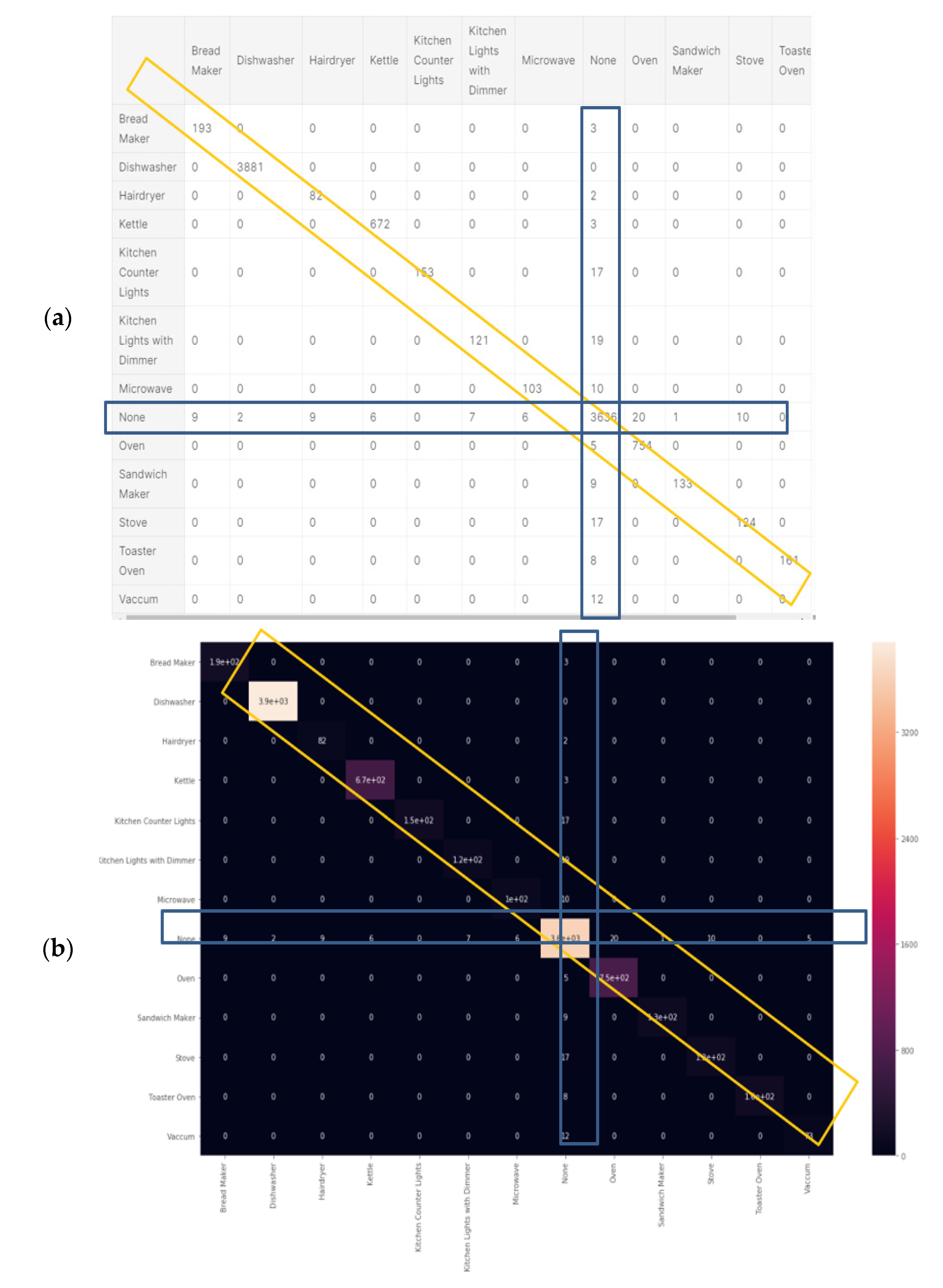
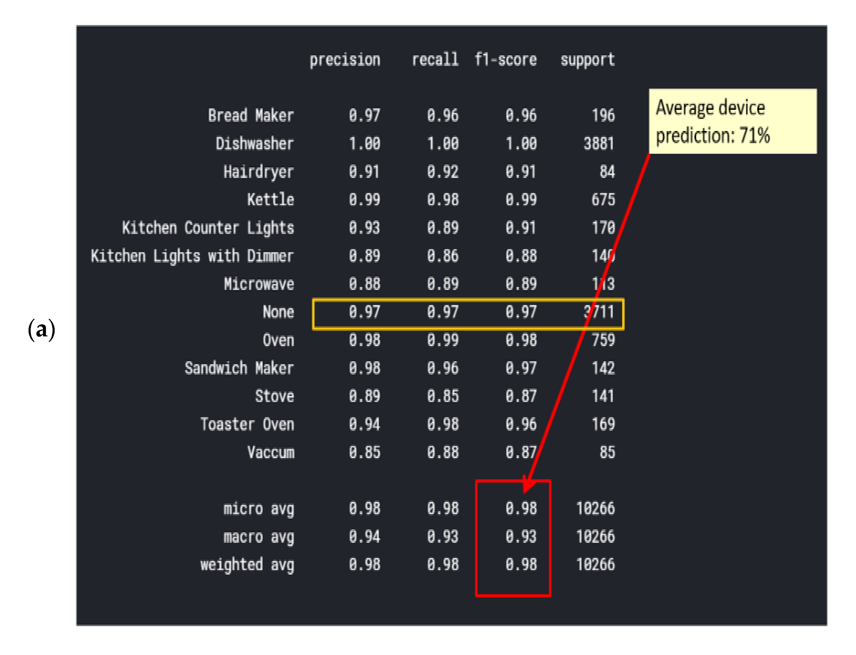
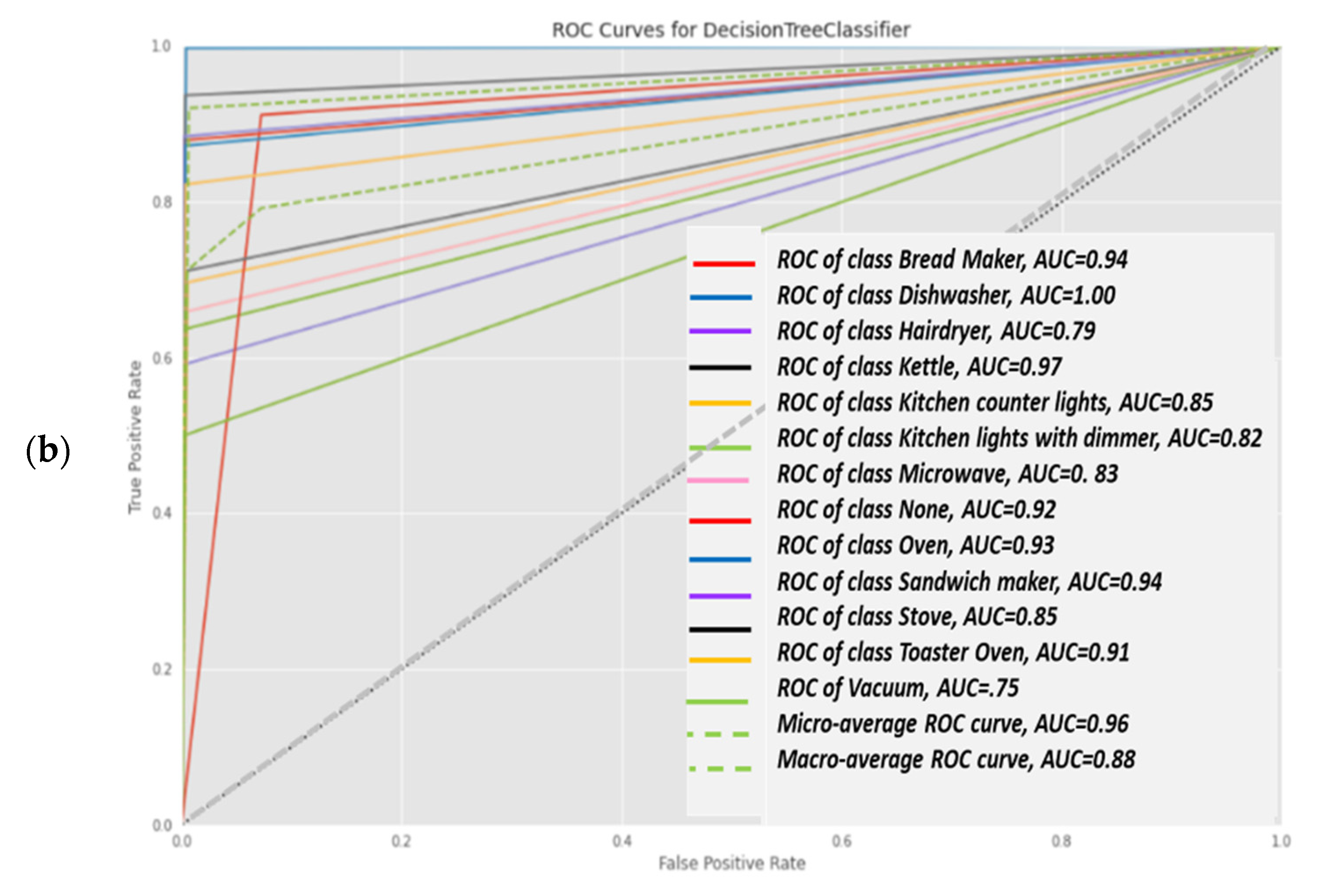
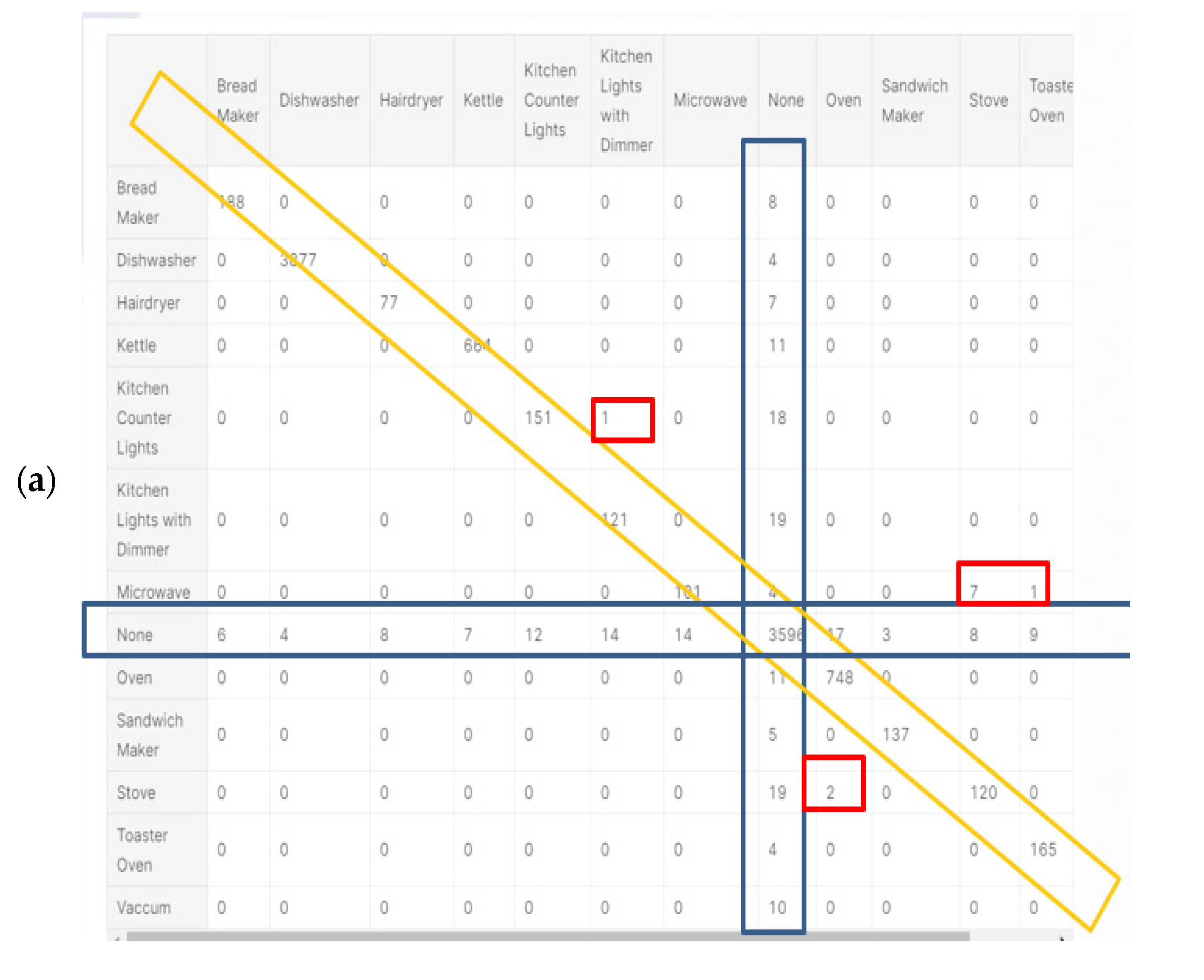
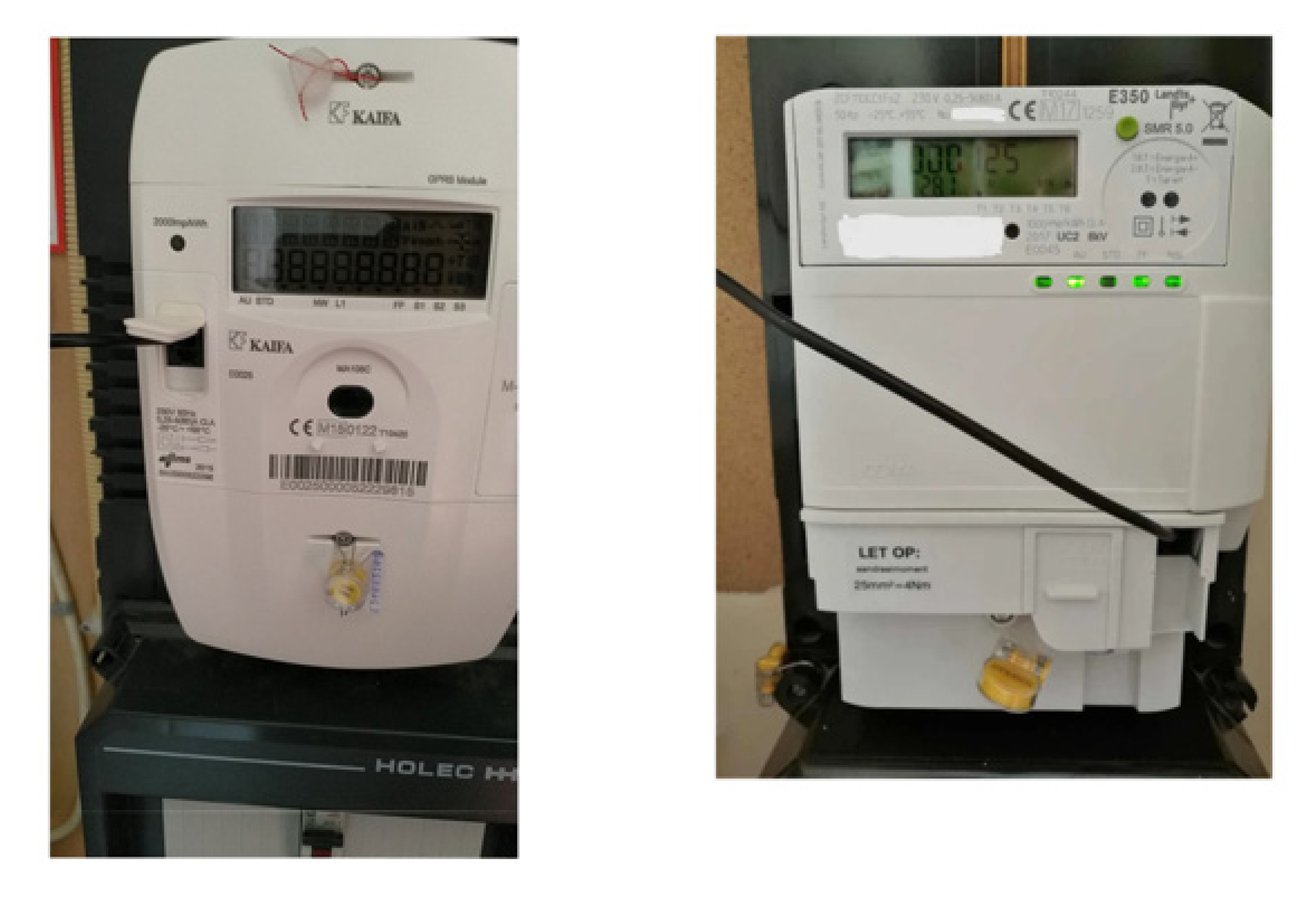
Publisher’s Note: MDPI stays neutral with regard to jurisdictional claims in published maps and institutional affiliations. |
© 2021 by the authors. Licensee MDPI, Basel, Switzerland. This article is an open access article distributed under the terms and conditions of the Creative Commons Attribution (CC BY) license (https://creativecommons.org/licenses/by/4.0/).