Abstract
In recent years electricity sectors worldwide have undergone major transformations, referred to as the “energy transition”. This has required energy planning to quickly adapt to provide useful inputs to the regulation activity so that a cost-effective electricity market emerges to facilitate the integration of renewables. This paper analyzes the role of system planning and regulations on two specific elements in the energy market design: the concept of firm capacity and the presence of distributed energy resources, both of which can be influenced by regulation. We assess the total cost of different regulatory mechanisms in the Brazilian and Mexican systems using optimization tools to determine optimal long-term expansion for a given regulatory framework. In particular, we quantitatively analyze the role of the current regulation in the total cost of these two electricity systems when compared to a reference “efficient” energy planning scenario that adopts standard cost-minimization principles and that is well suited to the most relevant features of the new energy transformation scenario. We show that two very common features of regulatory designs that can lead to distortions are: (i) renewables commonly having a lower “perceived cost” under the current regulations, either due to direct incentives such as tax breaks or due to indirect access to more attractive contracts or financing conditions; and (ii) requirements for reliability are often defined more conservatively than they should be, overstating the hardships imposed by renewable generation on the existing system and underestimating their potential to form portfolios.
1. Introduction
Optimization and simulation models are often used in energy policymaking to portray future system scenarios, used as a basis for the definition of long-term policy goals and the most economic investment pathways to them [1]. The idealized optimization and simulation models used by policymakers, system operators and scholars to represent and study the electricity sector tend to agree that the fundamental objective of electricity system planning is to pursue the minimization of the total cost of the system (or, equivalently, maximizing total social welfare)—despite differences in terms of representation and solution strategy. Generally speaking, the problem of optimizing system expansion involves choosing the best possible mix of technologies to meet system needs. Knowledge of how well each technology’s physical attributes align with those needs is thus at least in principle sufficient to determine the desirability of investing in that particular technology.
There are many pathways through which new generators may come into the system: enabled by the spot market directly, free market bilateral contracting [2], long-term centralized auctions [3] and direct consumer-side investment. All methods have their strengths and potential weaknesses and therefore, regardless of the main strategy that a country picks for organizing system expansion, there is the potential for efficient or inefficient outcomes. In an efficient market that follows this ideal cost minimization objective, the role of regulation is simply to facilitate the most socially desirable outcome coming to fruition: for example, by minimizing transaction costs, correcting market failures or externalities and making sure agents have the proper incentives. In practice, however, regulatory design is a challenging task, and it is possible that regulations may yield less than ideal outcomes by introducing distortions in the market and in the contracting routes.
Indeed, in the context of a rapidly changing electricity sector, it is possible that regulations may not evolve fast enough to adapt to the new reality—for example, by using outdated assumptions to address system needs and technological contributions, therefore leading to a non-optimal expansion. Sometimes, market distortions are intentionally made in order to promote specific technologies, such as distributed generation, renewable energy or “strategic” projects such as reservoir hydro or nuclear. Intentionally or not, most regulation and reforms lead to some impact on the market agents’ perceived cost and, therefore, on the development of the system [4].
In recent years, the electricity sector has undergone major transformations, often referred to as the “energy transition”. There is an increasing role for variable renewable energy resources and for distributed demand-side services, as well as a strong incentive for net-zero scenarios [5]. Therefore, policy makers are responsible for ensuring that long-term energy targets are achieved without compromising the system’s reliability and safety, and that the long-term costs of the energy transition are appropriately assessed [6]. Nevertheless, it seems likely that in some countries regulations may already be operating more as an obstacle to optimal system expansion than as a facilitator as intended. Even if regulators are fully benevolent, given the rapidly changing context, it is easy for regulation to lead to inefficient expansion due to assumptions that are simply out of date. Additionally, the regulatory process is further complicated in practice by the existence of legacy costs that need to be recovered, legacy contracts and commitments that need to be honored and special interest groups that may attempt to influence policymakers.
This paper analyzes the role of regulations regarding firm capacity and distributed energy resources in guiding long-term system expansion by comparing the outcomes in terms of total system cost of current regulatory practices in Brazil and Mexico to a reference “efficient energy planning” scenario. In terms of firm capacity, the “efficient energy planning” criterion involves ensuring that the system’s total generation supply is at least three standard deviations greater than demand at all times as a reliability criterion (“three sigma” rule). This criterion was implemented as an iterative process in the optimization tool for determining optimal generation system expansion, repeated until convergence was reached at the desired reliability level. In terms of distributed generation, the “efficient energy planning” representation involves simply eliminating cross-subsidies and other regulatory benefits for adopters of these systems, and thus ensuring that adopters are truly motivated by their individual preferences and not external motivations.
With this quantitative exercise, we show that renewables commonly have a lower perceived cost under the current regulations, either due to some direct incentive or due to indirect access to more attractive contracts or financing conditions—not only in the case of distributed generation but also for centralized generation applications. Furthermore, we find that requirements for reliability are often defined more conservatively than they should be, overstating the hardships imposed by renewable generation on the existing system and underestimating their potential to form portfolios.
2. Materials and Methods
2.1. Core Methodology
This section describes the core methodology used to model the system’s long-term equilibrium for both case studies (Brazil and Mexico), which is the basis of this paper’s methodology for quantitatively determining the impacts of regulatory practices. In summary, the authors use a combination of the three simulation and optimization modules: (i) distributed generation, (ii) reliability and (iii) expansion and operation. Together these modules envision a minimization of the system’s total costs, while ensuring the predefined reliability requirements. Each module’s methodology, as well as inputs, adopted for the efficient scenario and regulatory constraints, will be further detailed throughout the chapter. It is worth highlighting that the representation in each of these modules can be affected by regulations—as a country’s policies change the methodology for assessing different technologies’ contribution to system reliability, change incentives that end consumers may perceive for adopting distribution generation, and/or change the “perceived cost” different system expansion candidates by offering preferential tax treatment and/or financing.
The main goal of the present paper is to address how the regulations currently implemented in Brazil and Mexico would lead to deviations in the long-term equilibrium relative to an idealized “distortion-free” scenario. Finding the “true” distortion-free expansion result is evidently a challenging task, and even though the present paper provides a robust methodology for these benchmarks, methodological refinements could be implemented as potential future work. Nonetheless, it seems undeniable that regulatory practices in many countries incorporate significant deviations from an “ideal” representation, due to political influence, legacy contracts, methodological simplifications, lack of data and other reasons—see, for example [6,7].
Figure 1 illustrates the general scheme of the methodology adopted, highlighting all modules and connections between them.

Figure 1.
General scheme of the methodology adopted.
2.1.1. Distributed Generation Module
Assuming efficient price signals, the market equilibrium achieved from utility-maximizing agents would be equal to the result of a cost-minimization problem—which would allow these small-scale solutions to be simply incorporated into the optimization model as an additional expansion candidate. However, regulatory incentives to DER tend to result in consumers perceiving radically different price signals compared to what the dispatch model suggests. Therefore, distributed energy resources (DER) adoption by individual consumers needs to be considered separately from the optimal system expansion.
In this paper, the authors have implemented an iterative process that aims to simulate the interactions between DER adoption and market-driven system expansion [8]. The adoption decision was based on a payback-based adoption curve, which is a methodology vastly used in the existing literature [9,10]. The “payback” represents the number of years until the system “pays for itself”, considering the upfront cost of the distributed generation system and the yearly benefit corresponding to the avoided cost of purchasing electricity from the grid at the electricity tariff. The smaller the payback, the more economically attractive the distributed generation investment, and therefore the higher the share of consumers that will ultimately choose to adopt this alternative.
2.1.2. Reliability Module
For the reliability module in the “efficient energy planning” scenario (that is, in the absence of regulatory distortions), the authors have selected the “three sigma” (3σ) criterion, which ensures that the system’s total generation supply is at least three standard deviations greater than demand at all times. Assuming a normal distribution of the net supply, the 3σ criterion leads to a probability of 99.7% of being able to supply the demand without issue.
In order to ensure that the supply would meet the 3σ criterion, an iterative process was implemented. For the first run of the model, an initial expansion with no reliability restriction was used. Then, the variability of the net demand (demand minus renewable generation) was measured and compared to the firm capacity of the system—as defined by the regulation of each country and further detailed in Section 2.5. If the criterion was met, the optimization stopped, otherwise the contribution of the renewable technologies would be recalculated based on the results and adjusted for the next iteration. At each iteration, the expansion and dispatch model is called, and the same analysis and check of the 3σ criterion is carried out. If the criterion is met, the optimization stops, otherwise a new iteration begins.
2.1.3. Expansion and Dispatch Module
In liberalized competitive electricity markets, system expansion is driven by generators acting with the goal of maximizing their own profits. Using standard microeconomic competitive market assumptions, the system expansion induced by market equilibrium of these profit-seeking agents would be equal to the one chosen by a central planner seeking to maximize total welfare [11,12]. Based on this fundamental principle, it is possible to estimate the generation system expansion in a liberalized market environment through a specialized computational tool that determines the minimum cost expansion plan for an electrical system.
For the simulations, the authors used a long-term expansion planning model that determines the least-cost decisions for the construction, retirement and reinforcement of generation and transmission projects. This optimization model is integrated with a dispatch simulation tool that represents the details of the production of all plants in the system, taking into account operational flexibilities and constraints and ensuring that supply and demand remains balanced at all times (a requirement of the electricity network). In this manner, the model optimizes the trade-off between investment costs to build new projects and the expected value of operative costs obtained from the transmission-constrained dispatch model [13,14].
One important aspect of the model that should be highlighted is that the hydrological and renewable generation uncertainties are handled explicitly with a stochastic Monte Carlo representation followed by the stochastic optimization of the utilization of the system’s resources. In practice, hourly renewable energy stochastic scenarios gathered from georeferenced databases along with historical hydro inflows are fed to a statistical model in order to obtain correlated probability distributions for various locations and renewable resources, which in turn are used to produce the representative stochastic series used by the optimization software.
The representation of system dispatch involves an hourly resolution of the supply-demand balance—a particularly important feature in scenarios with high renewable share, representing operational constraints within each day. The model represents chronological links between the seasons (representing the management of hydro reservoirs between wet and dry seasons) but not between years, where a “cyclic” representation ensures that volumes stored at hydro reservoirs in the beginning of the year must coincide with volumes at the end of the year for each scenario.
Overall, this simulation approach, with the chronological decision-making, the stochastic modeling of hydrology and renewable generation, the hourly temporal granularity, among others, is compatible with recommended reference methodologies for energy planning—and, more specifically, for energy planning in the context of the energy transition [6].
2.2. Expansion Optimization Paradigm
As a benchmark for the system expansion planning, the analysis considered a reference year whose demand is twice the current demand, where the system portfolio resulting from the expansion model would be operated to meet this required load in a “steady state” (or “static”) manner in the very long term. Note that, considering a demand growth rate of 2% per year, for example, our demand benchmark would be reached in 35 years (~2055), whereas with a growth rate of 4% per year, this benchmark would be reached within 18 years (~2038). Therefore, for ease of reference, we have considered the reference horizon of the simulations to be representative of year 2040. It should be highlighted that the proposed system expansion methodology only looks at the target year, building the entire amount of new capacity needed at once to meet the target demand. This is not entirely realistic in practice, seeing that the ultimate expansion outcome may depend on the incremental decisions made in each of the intermediate years—this notion of path-dependency can be especially prominent in a context of sharp changes over time (such as cost decreases, regulatory changes and phase-out of policy incentives). Nonetheless, analyzing the “optimal” long-term system breakdown without these path-dependency constraints can yield interesting insights about the systems. It should also be noted that, in order to allow maximum flexibility in the choice of expansion technologies, it was assumed that most plants of the existing system can be decommissioned—they would be replaced by the construction of new ones, if this is economically desirable given the least-cost criterion.
Furthermore, in order to reduce the computational effort required by the expansion problem while maintaining a detailed hourly resolution representation, the concept of seasons and typical days was used in the modelling. The first step of this strategy consists of grouping the months of the year into sequential seasons—in this analysis, standard seasons with a length of three months each were used. All “weekdays” were grouped together as one representative day, and all Saturdays, Sundays and holidays as a second “weekend” type representative day—taking into account that, within each season, all days that belong to each of these two categories tend to be not so different from one another and thus can be represented as being drawn from the same probability distribution. Even though refinements could be added (in particular, a distinction between Saturdays and Sundays), the authors found that the impact of such refinements on the optimization results was extremely minor.
Regarding the role of regulation, first of all we assume that regulations are carried out under conditions of perfect competition, which implies that the optimal solution from the expansion model can be interpreted as resulting from market equilibrium between generators competing in the electricity market [11,12]. From this construction, the optimal system expansion from the central planner’s perspective is the same as the competitive market equilibrium, and the role of an efficient regulatory design would be simply to minimize “frictions” in order to ensure that this optimal outcome would be reached. However, regulatory initiatives can also introduce frictions and distortions, which the authors represent using two alternative approaches (which together can account for the impacts of most regulatory implementations):
- Changing the perceived costs of specific technologies: making them appear cheaper or costlier than they actually are for the purpose of system expansion decisions due to subsidies or surcharges, respectively; or
- Introducing new constraints in the optimization problem.
In both cases, the optimization model is used to find a new equilibrium expansion strategy, and the cost of the modified optimization problem is expected to increase with the introduction of these policies.
2.3. Modeling of Candidates for System Expansion
Five key representative technologies were used as candidates for the system expansion:
- (i)
- Utility-scale solar power plant (assumed to have one-axis tracking);
- (ii)
- Utility-scale wind power plant;
- (iii)
- Combined cycle gas-fired plant, highly efficient but with a preference for a more predictable dispatch profile (CCGT);
- (iv)
- “Peaker” type gas-fired plant, prioritizing operational flexibility over thermal conversion efficiency (OCGT); and
- (v)
- Battery storage technology.
The candidates’ attractiveness for system expansion in the absence of special regulations was determined from a purely economic standpoint, and the optimization model determines whether their investment costs, fixed costs and operating variable costs are compensated by their corresponding benefit to the system (based on avoided costs of dispatching costlier plants and avoiding electricity shortages). The final parameters were based on international benchmarks, especially “Lazard’s Levelized Cost of Energy Analysis—Version 12.0” [15] and “Lazard’s Levelized Cost of Storage Analysis—Version 4.0” [16].
Even though solar and wind technologies have been observing a continuous decreasing price trend for several years [17], there is a significant degree of uncertainty with regards to how long this trend may continue and therefore a conservative assumption of not representing any additional cost decreases in the long-term expansion was used. For battery storage technology, on the other hand, a decreasing cost curve was considered—since the technology is currently not sufficiently cost-competitive for large-scale applications in the electricity sector and it is at a much earlier stage in its technology life cycle than wind or solar, suggesting it still has ways to go before achieving maturity. Synergies with other economic segments (such as consumer electronics and electric vehicles) are also likely to contribute to pressuring battery prices downwards. The battery candidates were modeled as batteries with 4 h storage capacity at a long-term cost circa 60% lower than the average current price from Lazard (same cost in both case studies). Additionally, for transmission, only the main corridors between regions were represented, using the distance between the regions and a cost benchmark in USD/km for high voltage networks in order to estimate the cost of expanding interconnection capacity as an additional candidate technology for the expansion model.
Ultimately, Table 1 and Table 2 summarize the assumptions for each technology used in the analysis for the two countries.

Table 1.
Assumptions for expansion technologies in Brazil.
Table 2.
Assumptions for expansion technologies in Mexico.
In order to properly represent the maximum generation potential for renewable energy sources along with the corresponding profiles, a plurality of potential plants was created based on wind and solar scenarios from different locations with various resource quality levels. Typically, the quality of resource becomes a limiting factor as a greater amount of total capacity is developed: the best available areas tend to be developed first, though in practice, in our simulations the potential was very rarely completely exhausted. Figure 2 and Figure 3 illustrate the different representative wind generation daily profiles (pictures on the left, representing the average profile over 24 h and highlighting regional variabilities), the zones with high wind potential (pictures in the middle, color-coded to represent the quality of the resource) and high solar potential (pictures on the right, similarly color-coded) in each country.
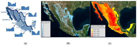
Figure 2.
Wind profiles (a) and zones with high wind (b) and solar (c) potential in Mexico.

Figure 3.
Wind profiles (a) and zones with high wind (b) and solar (c) potential in Brazil.
It is also crucial to properly represent the uncertainty and variability of renewable energy sources and in particular, the historical correlations among hydrology, wind, solar and other variables in the power system in order to properly incorporate portfolio effects into the optimization. These spatial dependencies were modeled through a Bayesian network, which automatically identifies the dependency relationships between the various time series of interest [18]. The result is a set of coherent probabilistic scenarios for the resource availability of inflows and renewables that can be used for the calculation of the stochastic operation policy with hourly representation.
Fuel prices are another key driver of electricity prices and are an extremely relevant input for system expansion decisions, since they directly impact the operational cost of thermal power plants and, consequently, their competitiveness with other technologies. The opportunity costs of hydro power plants are also highly affected by fuel prices, though indirectly. Generally speaking, if the domestic fuel market is efficient, fuel pricing should be driven mostly by the international fuel price—as this represents a “netback” price at which fuel can be imported or fuel surpluses can be exported. Therefore, a direct relation of fuel prices with international dynamics is assumed for all fuels in the efficient energy planning scenario. In order to ensure that long-term international fuel price forecasts are coherent (despite the inherent uncertainty given in the long-term horizon of the analysis), the projections of the U.S. Energy Information Administration (EIA) were adopted as a reference to the international price dynamics, taking 2040 as a base date [19]. This assumption leads to a long-term gas cost in the USA (Henry Hub, USA) of 4.3 USD/MMBtu in the long term (in the reference year 2040).
It is necessary to further incorporate additional costs for transportation, losses and similar services that must be considered in the final price of natural gas. In Brazil, the natural gas that sets the marginal price for gas-fired expansion is imported via LNG, which leads to an assumption of loss factor of 15% and additional costs of 3 USD/MMBtu—yielding a final gas price of 7.3 USD/MMBtu to be used in the simulations. In Mexico, in turn, Henry Hub natural gas is typically imported via pipeline, leading to negligible losses and additional costs (in line with what is reported by PEMEX) of approximately 1.65 USD/MMBtu—yielding a final gas price of 5.95 USD/MMBtu.
Regulatory Constraints
Under the efficient energy planning scenario, the attractiveness of each technology is evaluated based on its levelized cost. However, it is possible for regulation to introduce distortions that may result in a perceived cost for certain technologies that can be different from their true cost—usually through some type of (direct or indirect) incentive or subsidy. Generally speaking, a technology with a perceived cost that is higher than its true cost is disincentivized and becomes less likely to be built, while conversely a technology with a perceived cost that is lower than its true cost is incentivized and becomes more likely to be built—increasing the likelihood of suboptimal system expansion choices and cost overruns.
For this analysis, the notion of the pre-tax weighted average capital cost (WACC) was used to represent the financial attractiveness of a particular investment by evaluating only the project’s (pre-tax) cashflow. The WACC consolidates information on financing and taxation, allowing cost-benefit analyses to be made on the project’s cashflow directly without requiring further assumptions on company strategy, cost of debt and other parameters. For the purpose of the efficient energy planning scenario, all generation sources had the same WACC of 9% per year. For the current regulation scenario, however, typical market practices were used to estimate a perceived WACC that is allowed to vary for each technology [10].
In Brazil, investors and financiers have long required higher interest rates for infrastructure projects when compared to Mexico, which translated into a higher WACC. The role of these uncertainties in increasing the WACC, however, is offset in terms of perceived cost by the availability of cheap loans by Brazilian public banks for renewable projects. In Mexico, renewables tend to be favored by the current contracting mechanisms, since they have been the only ones allowed to offer all three products in the long-term auctions, which is one of the most relevant drivers to the system expansion and the other mechanisms do not introduce important distortions. This is reflected as a lower perceived cost for these technologies. Additionally, from the results of the auctions that have taken place in the country, it is possible to infer very low WACCs.
Market information on typically practiced debt-to-equity ratios, interest rate on debt and price practices in previous auctions were used to calibrate the generators’ perceived WACC. In this analysis, the main differences identified were that renewable projects that were able to secure long-term contracts in auctions and had special conditions for loans tended to achieve higher leverage ratios (higher D/E) and lower return rates—both from the financier (debt) and from the sponsor (equity). Conversely, in a similar analysis, higher WACC rates were identified for thermal projects, mainly driven by the restrictions to the contracting alternatives available to them. The final pre-tax WACC in the efficient scenario and in the current regulation scenario is presented in Figure 4.
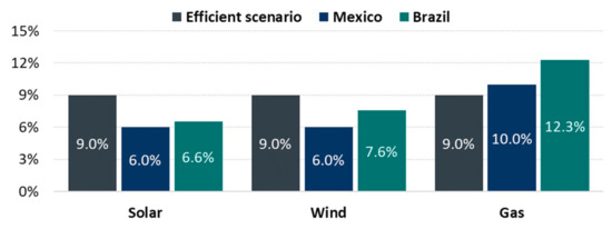
Figure 4.
Pre-tax WACC for Brazil and Mexico in the current and efficient regulation scenarios.
2.4. Distributed Energy Resources Expansion
Distributed generation is playing an increasingly important role in modern electricity systems, and thus it merits evaluating to what extent regulation may be facilitating (or making things difficult) for this type of consumer-driven initiative to flourish. Regulation is necessary to ensure that consumers with distributed generation (DG) facilities are properly rewarded for the energy they provide to the grid, and in an efficient energy planning scenario the incentive passed through to consumers is equal to the benefit that these installations provide to the grid—which in turn depends on their generation profile and on their role in reducing costs of transmission, if applicable. It is worth highlighting that the methodology used in our assessments was limited to solar distributed generation, which has achieved a degree of maturity that allows for modeling adoption with a reasonable level of accuracy. It would be possible, however, to extend the methodology or several other types of distributed energy resource.
In order to estimate the DER expansion, a payback-based adoption curve was used, following practices commonly adopted in the existing literature [9,10]. Generally speaking, DER plays a role whenever it becomes desirable for individual consumers to invest in their own system rather than purchasing electricity from the grid, which is incorporated into the payback metric (representing the number of years necessary to recoup the initial investment due to their monthly savings on the electricity bill). Even though this decision can be different for each individual consumer, in aggregate the share for the market will adopt a larger amount of DER units if the payback is lower (implying that the system pays for itself in a relatively short time). The analysis was focused on small-scale solar systems (assuming a mix of residential, commercial and industrial systems), which tend to be the most prominent DER adopters, with significant market penetration even today. Figure 5 illustrates a range of possible adoption curves, as compiled by Sigrin [9]. The vertical axis shows the total market share ultimately achieved by distributed generation as a function of the payback on the horizontal axis.
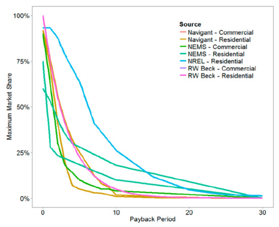
Figure 5.
Possible adoption curves as compiled by Sigrin (2016) [9].
The analysis considered the “RW Beck” curves as the key benchmark, which follows the simple exponential formula represented in Equation (1). Note that this methodology is in line with what has been commonly used by EPE (the planning entity in Brazil) in their forecasting studies—and, even though slightly different “payback sensitivity” parameters have been tested based on actual adoption data in different consumer classes in Brazil, in practice they deviate little from the 0.3 benchmark [20,21].
Even though, by assumption, all consumer classes were represented as having the same adoption curve, they perceive different payback levels, which created heterogeneity within each market.
Even though the solar generation technology is well-known for being relatively modular, meaning that economies of scale are less significant than with more traditional generation sources, residential-scale systems still tend to be around 25% costlier than commercial-scale systems, which in turn tend to be around 10% costlier than utility-scale systems (though with significant variations on those ratios). This is illustrated, for example, by comparisons of the cost of a utility-scale solar system (several thousand kW), a commercial-scale system (a few hundred kW) and a residential-scale system (a few kW) in different regions, as obtained from IRENA’s renewable energy cost database [22] and illustrated in Figure 6.
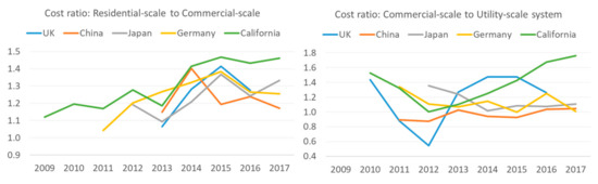
Figure 6.
Comparisons of the cost of a utility-scale solar system, a commercial-scale system (a few hundred kW) and a residential-scale system in different regions (authors’ analysis based on IRENA’s renewable energy cost database) [22].
Additionally, rooftop solar implementations also have lower performance on average than utility-scale ones, as they tend to undergo cleaning and maintenance less frequently and to have suboptimal orientation towards the sun (as they usually use the roof’s inclination to save on the cost of the structure). In the modelling, an additional 7% loss in the performance ratio was assumed for commercial-scale rooftop systems and a 15% loss for residential-scale systems (when compared to utility-scale) in addition to the higher costs described earlier to estimate the payback of those system sizes. This differentiation is applied on top of the regional differentiation based on the quality of the solar resource (which also affects payback).
Finally, the most important component for the analysis of the effect of regulation is the electricity tariff perceived by different consumer classes. The representation of “current regulations” in each of the reference countries was based on historical tariff data of each consumer class, and an “efficient regulations” scenario was constructed by applying multipliers that seek to represent whether consumers are able to offset a payment in USD/MWh that is higher than the true benefit of their DG installations for the system. The main goal of these multipliers is to capture the effect of regulations on the price incentives perceived by potential adopters even in the long term as system expansion and marginal prices interact: for example, consumers that can offset costs corresponding to transmission and distribution cost components of the electricity tariff effectively benefit from a regulatory distortion, and the lack of time-of-use tariff distinctions also tends to benefit DG adopters as the share of solar power in the system increases. The idea is that each individual consumer makes the choice that makes the most economic sense for themselves (given their preferences), which if their incentives are efficient would be exactly in line with what would be optimal for the system as a whole (after incorporating all possible externalities, such as reducing technical losses in the distribution network). If regulations over-incentivize DG adoptions, however, the share of consumers that will opt for owning a distributed generation system will increase, with consequences for the system expansion decisions.
In our model, the adoption rate resulting from the payback curve determines a fixed amount of distributed generation capacity to be part of the final expansion (complemented by the decisions of the system expansion module). It is worth highlighting that, as a general rule of thumb, distributed solar generation tends to offset centralized solar generation in the optimal system expansion, as it has similar characteristics (such as a generation profile peaking around the midday hours). However, there are a few key differences between utility-scale solar and rooftop solar from a system planning point of view, which have been incorporated into the model’s parameterization. The first one is the location of the projects: distributed generation projects are usually located near load centers, while centralized projects tend to be placed in the locations with the best resource potential. The second is the lower capacity factor of the distributed generation projects, due to a less reliable maintenance of the solar panels and lack of solar tracking.
2.4.1. Regulatory Constraints: Brazil
Perhaps the most significant consequences of regulation on the DG market are felt when distributed generation allows consumers to offset not only the tariff corresponding to the costs of energy but also other costs such as transmission and distribution costs and system charges—which is the case for Brazil. In the Brazilian case study, another distortionary effect is that taxation of electricity in most states is also offset from consumers’ electricity bill in proportion to distributed generation, thus strengthening the incentive by a significant amount (around 35% given steep electricity tax rates). Adding together these contributing factors, the end result in terms of DG adoption under current regulations for Brazil is shown Table 3, both as a fraction of the demand within each category and converted into the corresponding total capacity that would be built (in total, the model suggests 6 GW of distributed generation capacity).
Table 3.
Adoption of distributed generation in the current regulation scenario by class and region in Brazil.
Overall, low-voltage commercial and industrial consumers present the most significant cost-benefit ratio and therefore they are the ones with the highest distribution generation adoption levels—though the residential market, due to its substantial size, still accounts for most of the capacity additions according to this model. Medium-voltage consumers have a two-part tariff, and the capacity portion (proportional to peak demand) is in nearly all cases unaffected by the installation of distributed generation, as they typically occur at night.
2.4.2. Regulatory Constraints: Mexico
In Mexico, there are also regulatory incentives that reduce the payback of the distributed generation systems as perceived by end consumers (though not as profoundly as in Brazil). There is a program for residential consumers and small and medium-sized enterprises that provides an economic incentive equivalent to 10% of the total cost of the system, with the remaining 90% financed with FIDE resources, whereas for the agricultural sector the Shared Risk Program grants up to 50% of the value of the generation projects. There is also a support program for low-income families for the installation of ecotechnologies such as photovoltaic systems, among other initiatives [23]. Additionally, public policies have been implemented to guarantee open access, not unduly discriminatory against distributed generation. However, this policy seems to follow a reasonable economic rationale and offers no undue benefits—as the reinforcements of distribution network necessary for connecting distributed generation plants whose capacity exceeds the current limits of the maximum allocation capacity determined by the distributor will be borne by the applicant.
Distributed generation is also directly related to the tariff level in Mexico. Even though prior to the tariff reform in 2018, tariffs had been set below marginal price (thus disincentivizing rooftop solar), they have been readjusted in 2018, becoming more cost-reflective. It should be noted that, although a “Time-Of-Use” tariff (distinguishing between base, intermediary and peak hours) is available for large consumers from the industrial and commercial sectors, most low-voltage consumers typically only perceive an average monthly tariff that is applied equally to all hours. As a consequence, these consumers may potentially overvalue distributed generation delivered at midday in case there is an oversupply of solar power (which is also contemplated in the payback variable in our model). As low-voltage consumers do not perceive a time-dependent tariff, they are likely to be overcompensated for generation delivered at midday hours (the benefit to the system as a whole is low if there is a sufficiently large solar installed capacity, but the low-voltage consumer will be remunerated according to the average tariff). Adding together these contributing factors, the end result is shown in Table 4, both as a fraction of the demand within each category and converted into the corresponding total capacity that would be built. In total, the model suggests 1.6 GW of equilibrium installed capacity of rooftop solar.
Table 4.
Adoption of distributed generation in the current regulation scenario by class and region in Mexico.
As in the case of Brazil, low-voltage commercial and industrial consumers in Mexico present the most significant cost-benefit ratio, thus being the ones with the highest distribution generation adoption levels—with the medium-voltage commercial market dominating the additions due to their size. Adoption levels are typically higher in the Central region, mainly motivated by a higher loss factor passed through to the tariff incentive. The residential sector, in turn, has the lowest incentive due to a combination of a relatively low tariff and higher investment costs.
2.5. Reliability Requirements
Contrary to most markets in classic microeconomics, where there is a possibility of short- to medium-term storage at various points of the supply chain, the electricity grid is very sensitive to fluctuations, and instability can provoke outages with substantial social impact. This characteristic implies that electricity systems must ensure that supply and demand are balanced at any given point in time, which in turn requires procuring some amount of excess capacity to protect against supply inadequacy. As renewables have been increasing their share in most countries at a very fast pace, this topic has been rapidly increasing in importance, as the variability of intermittent generation sources compounds with the uncertainty of variations in the non-controllable demand and equipment outages to potentially increase the system’s need for robustness. In particular, several power systems have explicit regulations on “firm capacity” requirements (or similar metrics) to ensure that the system is operating with enough flexible dispatchable capacity to overcome even high-stress situations—typically implying high-demand hours in a high-demand season (potentially with additional contingencies). These regulations will be further detailed and modeled in the “current regulation” scenario for the Brazil and Mexico case studies.
In the “efficient energy planning” benchmark, the authors searched for a proxy for the ideal requirement level. Although this subject is broadly discussed worldwide, there is currently no absolute consensus among planning entities and system operators regarding the best methodology to calculate system needs in order to ensure reliability. Therefore, instead of using the explicit ad hoc constraints commonly applied by regulators and system operators, the authors sought to design a simple methodology from first principles that fairly represents the system needs even in a context of very high expected renewables penetration in the energy mix.
The main starting point is the principle of technology neutrality—that is, all technologies ought to be treated equally and their net effect on system reliability should be assessed exclusively based on (i) how much they contribute to increasing variance and uncertainty in the supply-demand balance (that needs to be accommodated by other units) and (ii) how much they contribute with flexibility that can be used to accommodate other agents’ uncertainty. Note that the neutrality principle used to guide the efficient energy planning representation is intuitive: if certain types of variability (e.g., climatic events such as El Niño) are treated differently from others, the system may prioritize these types of uncertainty (investing “too much” in being protected against these events) while possibly neglecting other sources of uncertainty, which means the system would not be as robust to these types of events. Therefore, the proposed methodology for calculating the system’s “efficient” reliability requirement focuses on the probability distribution of the net supply margin, defined as the difference between the available capacity and the net demand, and contemplating all possible sources of uncertainty equally. The net demand is defined as the demand discounted from the non-controllable renewable generation—in this study, the solar and wind generation, as per Equations (2) and (3). The index ω represents each scenario (or potential outcome) in the space of possibilities, seeing that these quantities are represented as random variables.
NetDemand (ω) = Demand (ω) − SolarGeneration (ω) − WindGeneration (ω)
NetSupply (ω) = AvailableCapacity (ω)−NetDemand (ω)
One common metric used in the context of system reliability analysis is the loss of load probability (LOLP) [24], defined as the probability that the net supply is negative (that is, the probability that the system’s capacity is insufficient to meet demand). Reliability requirements can be constructed based on this metric, by first defining a target LOLP level and calculating what is the minimum required firm capacity k to ensure this reliability level is met. Note that the firm capacity representation is necessarily a simplification, seeing that k is not a random variable (does not depend on ), even though in practice all technologies do involve some degree of uncertainty. It is straightforward, however, to check whether the reliability criterion is satisfied for all clusters (or groups of scenarios) , as depicted in Equation (6): if the probability is found to be much lower than for all , this is a sign that the system is oversupplied.
In practice, our methodology did not incorporate uncertainties in the available capacity (e.g., generator failures) into the representations of the joint probability distribution: dispatchable resources (such as thermal plants and batteries) were assumed to have negligible uncertainty and were represented as “pure” firm capacity values after discounting their expected unavailability rates. In practice, generator failures could have an effect in creating “fatter tails” in the probability distribution, and a more refined representation could be explored in future work.
Another key simplification made is to assume that, after properly subdividing scenarios into clusters (as will be described further), the LOLP within each cluster is chiefly described by the standard deviation of the probability distribution of net demand. This standard deviation, in turn, requires estimating the standard deviations and correlations between the individual components of net demand—namely, the demand side, solar output and wind output. Under this simplification, as depicted in Equation (7), it suffices for the expected value of net supply to be greater than three times its standard deviation (“3σ rule”) in order to ensure that the probability that net supply is greater than zero is at most .
In order to obtain consistent descriptions of the probability distribution of each component, the “clusters” for each scenario are defined by:
- (i)
- The season, which once again has known patterns for both demand and renewables; and
- (ii)
- The hour (highlighting daily profile patterns of demand and renewables).
Note that this paper focuses on weekdays for the presentation of the analysis of the variability of demand, though it would be straightforward to define an additional weekday versus weekend separation of clusters. There are, therefore, a total of 96 clusters (24 h and 4 seasons) modeled individually—each of which is represented individually. However, there is some structure to the time series data beyond pure classification into clusters: for example, two days in the summer of 2020 are expected to be “more similar” to one another than two days in the summer of different years, and the amount in hour 2 and in hour 3 of the same day are expected to be correlated despite belonging to different clusters. To account for this effect, the variation between samples of the same cluster are defined by three components, each of which is modeled as an autoregressive time series (that is, the “day” effect has some memory from the previous day, the “year” effect has some memory from the previous year, but they are otherwise unrelated):
- (i)
- The year, which may have a higher or lower than expected electricity demand (typically due to economic shocks or particularly harsh or mild summers or winters) and may also be subject to renewable resource effects (with hydrological multi-year cycles being notably pronounced);
- (ii)
- The day, which represents the fact that resource availability within each day is correlated across hours;
- (iii)
- The hour, which in practice represents a statistical residue (that is, the component of variation that cannot be explained by either yearly or daily correlations).
To make things intuitive, the aggregate supply margin will be broken down into separate timescale components in order to focus on each of those variables that describe the “clusters” of variability : the annual effect, the daily effect (between days after eliminating the effect of the year and season) and the residual effect (between individual hours after eliminating the hourly profile effect and other previous effects). The final net supply margin for each cluster is therefore a random variable equal to the sum of the random variables for each timescale component and each technology component (solar, wind, hydro and demand).
For each of the individual clusters, the total standard deviation is written as a sum of components representing contributions from the demand side or specific generation technologies (hydro, wind and solar) —the sum of all components yields . Note that there is a fundamental relationship between the second-order moments that allow for describing the standard deviation of the net supply as a whole by considering the variance , covariance , correlation and standard deviation of each of the components that add up to it. Equation (9) shows a derivation of this property, where represents the standard deviation of each component of net supply, represents the standard deviation of net supply as a whole (with ), and represents the coefficient of correlation between the component and the whole . Note that all equalities in Equation (9) are exact: the only key assumption required, as described earlier, is that the second-order moment is sufficient to describe the system’s reliability needs to a reasonable level of precision.
Note that the aggregation was made first among technologies within each timescale and then among timescales—the index in Equation (9) implicitly represents both types of aggregation. The sum, considering the covariances between the technologies and timescales, is the total variability that must be accounted for when designing the reliability constraint for efficiently guiding system expansion. A small additional caveat with regards to this representation is that the sequential nature of the optimization problem was imperfectly represented—each sample within each cluster is drawn from a probability distribution that may depend on the hours, days and years that came before it via autoregressive models, but when assessing reliability requirements in the long term, this correlation is not explicitly incorporated. This is in fact a reasonable approximation, seeing that at the expansion planning stage it is not possible to obtain special knowledge on short-term dynamics and it makes sense to consider a reliability criterion that weights all possible outcomes equally.
In summary, the impact of each timescale component and each technology was separated, and the covariance among these factors was calculated, reaching the total variability of the system’s net supply. This variability is then used to create the efficient reliability requirement, which should be met by the firm capacity in the system. A commonly used and reasonably conservative requirement involves a 3σ criterion, implying that the system’s expected excess supply (that is, total supply minus demand) is at least three standard deviations greater than zero in all clusters. If the probability distribution of the net supply was normally distributed, the 3σ criterion would yield a probability of being able to meet the demand without issue of 99.7%—reflecting a relatively conservative criterion. The probability distribution for the net demand could in principle be more fat-tailed, although in practice for very large numbers of generators and consumer units the distribution tends to approach the normal curve. It should be noted that, due to Chebyshev’s inequality [25], even if the true probability distribution had the worst possible shape, the 3σ criterion still ensures that the LOLP cannot possibly be higher than 11.1%—and it would be possible to apply a higher sigma (σ) multiplier in order to obtain even more conservative rules to add a “buffer” against more fat-tailed distributions. In order to comply with this 3σ requirement, the planning model utilized in this work was used with the analysis of the net supply margin in a loop, until convergence was reached.
In contrast to this “efficient” methodology for reliability requirements, which ensures that all technologies are treated in the same manner and only as a function of their variability parameters, different countries use very different approaches for defining reliability requirements. Despite these methodologies’ intent of promoting greater security of supply, a less than optimal methodology to define generators’ firm capacity (for example) can lead to inefficiency in the system expansion choices. An over-conservative criterion, for example, can lead the market to overcommit new capacity to attend reliability requirements, overcharging the consumer segment. On the other hand, an overly optimistic criterion or the lack of a proper periodic revision of firm capacities can lead to a serious violation of the system’s desired reliability levels. We discuss below the key aspects of the regulations currently applied in the two countries of the case study.
2.5.1. Regulatory Constraints: Brazil
In Brazil, the central focus of the institutional framework for planning of the electric system is the security of supply, which is guaranteed by two basic rules that are enforced on a 12-month basis: (i) every consumer must have 100% of its consumption covered by registered contracts [26]; and (ii) every contract must be backed up by a power plant capable of sustainably producing the contracted volumes, as measured by a “Physical Guarantee” value assigned to each power plant by the Ministry based on their physical characteristics [27]. In a simplified way, the physical guarantee calculation process of hydro and thermal generators can be summarized in two main steps. First, the maximum demand that the existing physical system can supply (according to a predefined security of supply criterion) is calculated. This number will ultimately correspond to the total sum of the physical guarantees of all plants in the system, ensuring that the system has a comfortable supply-demand balance (again according to the pre-established criterion) if and only if the system’s total physical guarantee is enough to cover the entirety of demand. Then, in the second step, the total physical guarantee is allocated among individual generation facilities.
For renewables, however, this approach is different—their contributions are calculated only for the plant itself without taking into account synergies with the existing system. The physical guarantee of wind power plants, for example, is calculated based on the energy expected to be yearly produced in, at least, 90% of years (P90), discounting the expected unavailability and losses up to the plant’s connection point [28]. The P90 value is assessed by a specialized company that certifies the wind measurements and associated calculations. For solar power, the methodology is similar, but the statistic used to determine the physical guarantee is simply the expected production value assessed by the certifying entity, rather than the more conservative P90 [29]. It should be noted that wind power physical guarantee is treated in a conservative fashion: a practice that could lead to overburdening consumers with the cost of too much unneeded extra capacity in the long term. On the other hand, reassessments of the robustness of the system as a whole are not carried out as often as they should be, and there is evidence that hydro plants have been generating less than their joint physical guarantees for several years [30]—possibly suggesting the opposite, that Brazil is being less conservative than it should be in its assessments of the country’s supply-demand balance.
Moreover, the Brazilian system is historically “energy-constrained” (as opposed to “capacity-constrained”) and the peak demand has easily been met with cheap instantaneous power provided by large hydro power plants. Therefore, all physical guarantee requirements mentioned are currently enforced only for energy production targets for the long term. However, as the penetration of renewables grows in the Brazilian electricity market, the requirements of peak demand supply are becoming more relevant due to the variable hourly pattern of these energy sources. In this context, developing security rules based on instantaneous power requirements may be a need in the near future, which is already on the regulator’s agenda. The concept of “peak physical guarantee”, focusing instead on ensuring that there would be enough capacity for generators to provide power during peak hours, was introduced in some early regulations and even contracts after the market reform in the early 2000s, though it has not been officially enforced. Using this regulation as a starting point, the modelling of the Brazilian current regulation scenario will include both a “Firm Energy” constraint (represented by the classic physical guarantees mechanism), which must be greater than average demand; and a “Firm Capacity” constraint (represented by the “peak physical guarantee”), which must be greater than peak demand. Figure 7 illustrates the concept of these constraints, as well as provides an estimation of the contribution of each technology to each criterion in terms of share of total installed capacity.
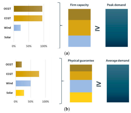
Figure 7.
Reliability constraints in Brazil: firm capacity (a) and physical guarantee (b) criterion.
2.5.2. Regulatory Constraints: Mexico
In Mexico, a distinguishing feature is the existence of a separate market for “capacity product” involving yearly settlements based on generators’ contribution in the 100 critical hours of each year, verified ex post [31]. The “yearly spot price” of capacity is calculated based on;
- (i)
- System-critical capacity margins calculated by the system operator;
- (ii)
- The cost of building a new peaker plant (calculated by the system operator using a reference thermal technology); and
- (iii)
- The surplus revenue that this reference thermal technology would have received selling its energy in the spot market under ideal conditions (which is discounted from the final capacity payment).
The yearly capacity payment is thus calculated to be complementary to energy spot market revenues, contributing to stabilizing generators’ yearly cashflows.
The Mexican capacity market has the key features of a regulatory reliability mechanism, by focusing on the ability to supply demand in the most extreme circumstances (as represented by the 100 critical hours). Interestingly, it does not operate as a “hard” constraint, but rather as the imposition of a “soft” financial incentive: if the minimum capacity margin drops below the minimum (defined as 7.7% in the current regulation), for example, generators would be allowed to recover twice their fixed costs, thus incentivizing the construction of new capacity capable of supplying the system during the critical hours. The end result of this incentive, therefore, is in a way similar to what can be achieved with “hard” firm capacity constraints, as it aims to incentivize a certain reliability level to be met. Figure 8 summarizes the price formation used for the mechanism. A curious feature of the Mexican reliability mechanism is that, because spot market revenues are used in the calculation, this means that generators may end up not receiving capacity revenues at all in years when the market is exceptionally tight (though they will still receive them during high-supply years). In practice, the adopted methodology accounts for the average expected capacity revenue (considering all types of supply-demand balance), which is expected to be the most reliable signal for system expansion.
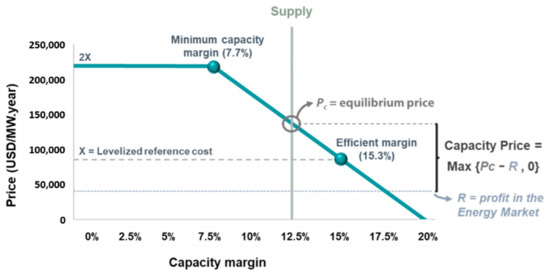
Figure 8.
Reliability constraints in Mexico: capacity market price formation.
Renewables are remunerated according to their measured output in the critical hours, whereas hydro and thermal plants are remunerated according to their availability (maximum potential output) at these same moments. In this sense, the Mexican reliability mechanism is relatively progressive, ensuring that (despite their stochastic nature) renewables’ contributions under critical conditions are valued by the mechanism. Despite this positive feature of all technologies being properly contemplated by the mechanism, the incentives put in place by the Mexican capacity market still tend to slightly favor conventional generators. For example, the fact that the price of capacity is dependent on the fixed cost and assumed energy market revenues of a peaker thermal plant in particular means that this technology tends to have less risk in its capacity market revenues. In addition, and perhaps most noticeably, hydro and thermal plants usually have their contributions during the critical hours equal to their available capacity even if they are not dispatched, whereas renewables have contribution equal to their actual generation—implying that they may be penalized if they need to be curtailed during critical demand hours (for example due to transmission bottlenecks or to accommodate ramping of thermal generators).
The Mexican capacity market was represented by altering expansion candidates’ “perceived cost” for choosing optimal system expansion. This was conducted by subtracting the expected capacity market revenues from the annualized investment cost for each technology. It should be noted that determining expected capacity revenues is an iterative process, as the capacity prices and the critical hours themselves shift depending on the expansion mix (which in turn is decided by the perceived costs of the technologies). In order to estimate this interplay, the modelling accounted for how system expansion alters the identification of which hours are likely to be considered “critical”. Following the current regulation, the firm capacity of renewable technologies was adjusted to reflect the expected generation in these critical hours, while for thermals and hydros it was assumed to be equal to their availability.
3. Results
3.1. Brazil Results
The final expansion mix, both in terms of capacity and share of the expansion, is summarized in Figure 9 for the two scenarios: efficient and current regulations.
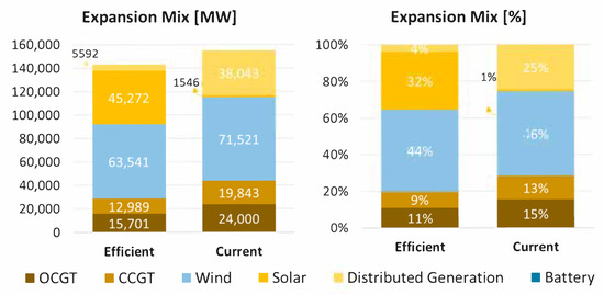
Figure 9.
Comparison of total expansion between scenarios.
The first point that stands out is the remarkably larger expansion of distributed generation in the current regulation scenario compared to the efficient energy planning one, caused by the numerous incentives to this source. Consequently, the utility-scale solar expansion is drastically reduced—for the most part it is substituted by the rooftop solar alternative, which has a similar production profile, but does not contribute to the system reliability criterion as detailed earlier. In contrast, wind technology increases its share in total expansion. Also noticeable is the higher share of natural gas sources in the current regulation scenario, motivated by the higher share of intermittent sources and by the regulatory reliability requirements. Battery capacity does not participate in any of the scenarios simulated—this is because the large amount of existing hydropower in the Brazilian system is already sufficient to shift demand between hours of each day, providing a service that in other systems would need to be delivered by batteries.
Another interesting comparison pertains to the expansion among electrical regions [32], as depicted in Figure 10. In both regulation scenarios, solar capacity is mostly concentrated in the Southeast region, since it has a great potential and is located close to demand; whereas wind capacity is greatly focused in the Northeast, where the highest capacity factors lie. Regarding natural gas, in the optimal scenario, this expansion is mostly concentrated in the South, while in the current regulation one, it is spread out among the regions. In addition, as the distributed generation potential is proportional to the regional demand, it is mostly concentrated in the Southeast.
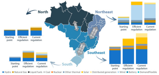
Figure 10.
Comparison of the regional expansion between scenarios.
It is also worth analyzing the impact of the distinct expansions in the system operation, which is depicted in Figure 11 and Figure 12. It should be noted that this figure represents only the average values for the main typical day of each season (typical weekday). Each scenario incorporates data on hydrological inflows (that vary by season) and solar and wind production (that varies hourly).

Figure 11.
Generation profile per season in the efficient regulation scenario.

Figure 12.
Generation profile per season in the current regulation scenario.
Notably, solar and wind generation, as relatively inflexible resources in the intraday period, are the “base” of the generation mix and usually require flexible sources to accommodate their daily pattern. This flexibility is chiefly provided by hydro generation, which fluctuates along the day to ensure energy balance, while thermal generation is very smooth during the day in this average profile. During season 3, for example, there is an almost 50 GW ramp in hydro generation in only a couple of hours caused by solar and wind power increment.
Subsequently, the reliability of the system is analyzed. For this analysis, the consultants compared the net demand (that is, demand discounted by renewable generation) and its variability with the total available capacity of the system, as presented in Figure 13. Remarkably, in both expansion scenarios the reliability margin is very close to the ±3σ criterion, indicating good equilibrium of supply-demand and a well-adjusted system. Nonetheless, the volatility of the net demand in the current regulation scenario is substantially higher when compared to the efficient case, caused by a greater wind and distributed generation expansion—which in turn implies a higher need for flexible thermal capacity.
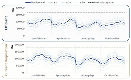
Figure 13.
Comparison of the system reliability level between scenarios.
Figure 14 and Figure 15 highlight the contrast between the two scenarios in terms of total cost needed to remunerate the existing generation system (only operational costs) as well as the system expansion represented. Note that the total social surplus perceived by consumers (from having their electricity demand met) may be shared among market agents in several ways—implicitly, whenever a given sector (such as transmission, generation or trading) receives positive profits, they are allowed to capture a greater share of this social surplus. However, as the regulations that govern this cost allocation across agents can be very complex and the number of assumptions required to make a long-term assessment is extremely high, the assessment of this idealized total cost view is limited to focusing on the aggregate outcome. The total cost is proportional to the area of the curve, with the width representing installed capacity of each technology and the height representing the cost per unit of installed capacity. Note that, generally speaking, because the expansion mix was selected by an optimization model, it is to be expected that costlier units also have proportionally higher contributions to system reliability and/or flexibility, justifying this higher cost. In addition, in order to allow the direct comparison between the efficient energy planning and current regulation scenarios, note that all costs represented reflect true costs (rather than perceived costs).
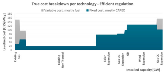
Figure 14.
Cost breakdown in the efficient regulation scenario. Total cost (variable + fixed) equal to USD 20.8 billion.
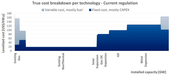
Figure 15.
Cost breakdown in the current regulation scenario. Total cost (variable + fixed) equal to USD 24.2 billion.
One main impact that stands out is the greater deployment of distributed generation and a drastic reduction in large-scale solar expansion in the current regulation scenario, when compared to the efficient energy planning one. Another remarkable point is the greater expansion of natural gas power plants, both open cycle and combined cycle. These differences resulted in greater investment costs and also in more pronounced operational costs. Overall, the regulatory distortions led to a 16% higher total cost than the one obtained in the efficient energy planning scenario.
3.2. Mexico Results
The final expansion mix, both in terms of capacity and share of the total expansion, is summarized in Figure 16 for the two scenarios: efficient and current regulation.
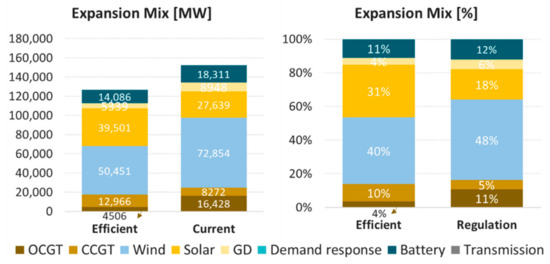
Figure 16.
Comparison of total expansion between scenarios.
Notably, the current regulation scenario promotes a significantly higher insertion of wind power and natural gas, both in terms of absolute capacity and in terms of share of the expansion mix. In contrast, due to the low recognized contribution of solar for regulatory firm capacity requirements in the long-term, this technology tends to have a reduced representation in the current regulation scenario. Distributed generation is also greater in the current regulation case, largely due to the existing incentives. Battery capacity and transmission capacity are also slightly higher in the current regulation scenario.
Another interesting comparison is among regional expansions, depicted in Figure 17. It seems that both the reduction in solar capacity additions and the increase in wind capacity additions affected all three regions in a relatively uniform manner, maintaining relative proportions with the North and South being more prominent in wind power and Central concentrating most of the solar capacity. The increase in the natural gas expansion in the current regulation scenario, on the other hand, is mostly concentrated in the North, even though there is also a perceptible increase in the South. As distributed generation is proportional to the regional demand, it is mostly concentrated in the Central region.
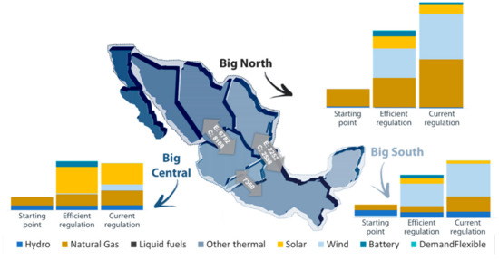
Figure 17.
Comparison of the regional expansion between scenarios.
The significant high-quality potential of wind in the North and South of the country leads to a great expansion of this technology in both regions. In the Central region, the less attractive wind resources, high-quality solar potential and proximity to the main load centers contribute to a greater solar expansion. Regarding natural gas, the expansion is mostly concentrated in the North, due to the easy access to cheap North American natural gas. There is also a significant expansion of gas in the Central region, as this is the region with the greatest demand and natural gas can help form a portfolio with the large amounts of solar power built. Also noticeable is the expansion of the interconnection lines between the North and the South and Central zones.
Another interesting output from the simulation is the daily profile of generation per technology, illustrated in Figure 18 and Figure 19. Most of the generation during the day is provided by wind and solar power plants, while at night natural gas becomes more relevant. It is also interesting that wind generation is higher in the night period—when demand is also more pronounced. Batteries play a role mostly by moving solar generation from the daytime (when supply is abundant) to the night period, reducing the need for thermal generation at night.

Figure 18.
Generation profile per season in the efficient regulation scenario.
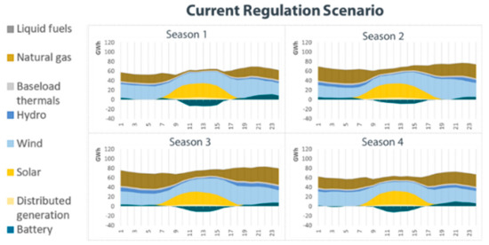
Figure 19.
Generation profile per season in the current regulation scenario.
Subsequently, the reliability of the system is analyzed. For this analysis, the net demand—demand with renewable generation discounted—and its variability is compared with the available capacity of the system, as presented in Figure 20. The system expansion obtained in the efficient regulations scenario remains very close to 3σ in all four seasons, meaning that the system is well-balanced for delivering the desired level of reliability. In the current regulation scenario, the system expansion obtained highly surpasses the 3σ criterion in all four seasons, reaching a level very close to 6σ—indicating a substantial oversupply driven by the incentives put in place by the current regulations.
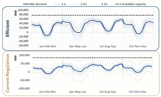
Figure 20.
Comparison of the system reliability level between scenarios.
Figure 21 and Figure 22 presented next highlight the contrast between the two scenarios in terms of total cost needed to remunerate the existing generation system for the Mexican case. The differences in expansion found, such as the higher overall amount added in the current regulation scenario, as well as its higher wind, natural gas (especially open cycle) and DG participation and lower solar generation, are translated into significantly higher total investment costs, though accompanied by a small reduction in the total operational costs largely due to the greater role of renewables. Overall, the regulatory distortions led to an 11% higher total cost when compared to the efficient energy planning case.

Figure 21.
Cost breakdown in the efficient regulation scenario. Total cost (variable + fixed) equal to USD 22.8 billion.

Figure 22.
Cost breakdown in the current regulation scenario. Total cost (variable + fixed) equal to USD 25.3 billion.
4. Discussion
For each of the two case studies proposed (Brazil and Mexico), the authors contrasted the system expansion in a “current regulation” scenario with the expansion in an “efficient energy planning” scenario, analyzing the results of the optimization model. In the “current regulation” case, the authors have modeled the main regulations that directly impact the system expansion. In the “efficient energy planning” case, on the other hand, the authors have used a proxy for “ideal” policies with regards to reliability requirements and distributed generation, which involves ensuring cost-reflectiveness of all technologies. The analysis highlights how the countries’ regulation impacts the systems’ expansion, in addition to how the physical features of the different markets play a role in the results. Our chief conclusion is that imperfections in the regulatory incentives for system expansion led to a deadweight loss of significant magnitude, in the order of USD 3 billion: the Brazilian case study indicated a 16% surcost in the current regulation scenario compared to the efficient regulations one, and the Mexican case study indicated an 11% surcost. These differences are attributed to a combination of the three effects assessed in the present paper: a distorted representation of expansion candidates’ perceived relative cost, a distorted incentive for adopters of distributed energy resources and a distorted representation of different technologies’ contributions to system reliability and/or the system’s reliability needs.
In Brazil, the current regulation led to a remarkably larger distributed generation expansion, caused by the numerous incentives to this source, and to substituting the utility-scale solar expansion from the efficient energy planning scenario. In contrast, wind technology increased its share in total expansion. Additionally, there was a higher share of natural gas sources in the current regulation scenario, motivated by the higher share of intermittent sources and regulatory reliability requirements. Battery capacity did not participate in any of the scenarios simulated, motivated by the large amount of existing hydropower in the system, which is already sufficient to shift demand between hours of a single day, providing a service that in other systems would be delivered by batteries. Another interesting comparison is among regional expansions: the natural gas expansion in the efficient scenario was mostly concentrated in the South, while in the current regulations one, it was spread out among the regions. These differences resulted in greater investment costs and also in more pronounced operational costs. Overall, the distortions attributed to the current Brazilian regulations led to a 16% higher total cost than the optimal scenario.
In Mexico, the current regulations scenario promoted a significantly higher insertion of wind power and natural gas, both in terms of absolute capacity and in terms of share of the expansion mix. In contrast, due to the low recognized contribution of solar for regulatory firm capacity requirements, this technology had a reduced representation in the current regulation scenario. Battery capacity was also slightly higher in the current regulation scenario. Also remarkable were the greater capacity additions of open-cycle natural gas, while combined cycle capacity was slightly reduced. These differences translated into significantly higher total investment costs, though accompanied by a small reduction in the total operational costs, largely due to the greater role of renewables. Overall, the regulatory distortions led to an 11% higher total cost when compared to the optimal regulation case.
Even though each system is different, both from a physical and a regulatory standpoint, the present work proposes a framework that makes it possible to make meaningful assessments of the role of regulation in a context of rapidly transforming electricity sectors, especially in terms of system expansion and planning. In particular, two very common features of regulatory designs in electricity markets (observed both in Mexico and in Brazil) are: (i) renewables commonly having a lower perceived cost under the current regulations, either due to some direct incentive or due to indirect access to more attractive contracts or financing conditions; and (ii) requirements for reliability are often defined more conservatively than they ought to be, overstating the difficulties imposed by renewable generation to the existing system and underestimating their ability to contribute. Together, these features tend to lead to an overcapacity situation, as the first driver seeks to purchase as many renewables as possible while the second one promotes contracting additional conventional generators to guarantee system firmness.
This impact is very noticeable in the results presented for Mexico, where the current regulation scenario led to an extremely conservative outcome in terms of reliability (as measured by the number of standard deviations between system net demand and firm capacity). In the case of Brazil, the current regulation also led to a higher total expansion, though interestingly not a more reliable system—as the higher capacity levels were counterbalanced by the higher variance of the expansion mix driven by current regulation. In both cases, although there is an incentive for the development of renewables, due to (i), there is also an incentive from the planning regulation for the expansion of thermal technologies from (ii)—as the contribution of renewables to system reliability is assumed to be very low and the regulation that defines the attributes of batteries or other storage technologies (for reliability and as a non-polluting technology) is still poorly developed. This indicates that planning regulations usually lead to a non-optimal expansion scenario, especially due to over-conservative requirements and the need for updates and revisions. Additionally, it raises an important obstacle to a net-zero scenario, which needs substantial changes in the regulation to be feasible in the analyzed systems.
Author Contributions
Conceptualization, G.C. and L.B.; methodology, G.C., A.W. and J.B.; software, J.S. and B.B.; validation, G.C. and A.W.; writing—original draft preparation, A.W. and G.C.; writing—review and editing, L.B. and A.W.; supervision, G.C.; project administration, A.W. and J.S.; funding acquisition, PSR Energy Consulting and Analytics. All authors have read and agreed to the published version of the manuscript.
Funding
This research received no external funding.
Institutional Review Board Statement
Not applicable.
Informed Consent Statement
Not applicable.
Data Availability Statement
Not applicable.
Conflicts of Interest
The authors declare no conflict of interest.
References
- Mai, T.; Logan, J.; Blair, N.; Sullivan, P.; Bazilian, M. RE-ASSUME: A Decision Maker’s Guide to Evaluating Energy Scenarios, Modeling, and Assumptions. International Energy Agency—Renewable Energy Technology Deployment. 2013. Available online: http://iea-retd.org/wp-content/uploads/2013/07/RE-ASSUME_IEA-RETD_2013.pdf (accessed on 9 August 2021).
- Lima, D.A.; Paula, D.N.T. Free contract environment for big electricity consumer in Brazil considering correlated scenarios of energy, power demand and spot prices. Electr. Power Syst. Res. 2021, 190, 106828. [Google Scholar] [CrossRef]
- Tolmasquim, M.T.; de Barros Correia, T.; Porto, N.A.; Kruger, W. Electricity market design and renewable energy auctions: The case of Brazil. Energy Policy 2021, 158, 112558. [Google Scholar] [CrossRef]
- Daglish, T.; de Bragança, G.G.F.; Owen, S.; Romano, T. Pricing effects of the electricity market reform in Brazil. Energy Econ. 2021, 97, 105197. [Google Scholar] [CrossRef]
- Soares, Í.N.; Gava, R.; de Oliveira, J.A.P. Political strategies in energy transitions: Exploring power dynamics, repertories of interest groups and wind energy pathways in Brazil. Energy Res. Soc. Sci. 2021, 76, 102076. [Google Scholar] [CrossRef]
- IRENA. Planning for the Renewable Future; International Renewable Energy Agency: Abu Dhabi, United Arab Emirates, 2017. [Google Scholar]
- Gonzalez-Romero, I.C.; Wogrin, S.; Gomez, T. Transmission and storage expansion planning under imperfect market competition: Social planner versus merchant investor. Energy Econ. 2021, 103, 105591. [Google Scholar] [CrossRef]
- Cunha, G.; Moreira, H. An Econometric Assessment of the Technological Innovation and Diffusion Model for Distributed Generation in Brazil. In Proceedings of the IAEE International Conference, Paris, France, 4–7 July 2020. [Google Scholar]
- Sigrin, B.; Gleason, M.; Preus, R.; Baring-Gould, I.; Margolis, R. The Distributed Generation Market Demand Model (dGen): Documentation; Technical Report NREL/TP-6A20-65231; National Renewable Energy Laboratory (NREL): Golden, CO, USA, 2016.
- Sigrin, B.; Drury, E. Diffusion into New Markets: Economic Returns Required by Households to Adopt Rooftop Photovoltaics. In Proceedings of the AAAI Energy Market Prediction Symposium, Arlington, VA, USA, 15–17 November 2014. [Google Scholar]
- Schweppe, F.C.; Caramanis, M.C.; Tabors, R.D.; Bohn, R.E. Spot Pricing of Electricity; Springer: New York, NY, USA, 1988. [Google Scholar]
- Ehrenmann, A.; Smeers, Y. Risk adjusted discounted cash flows in capacity expansion models. Math. Program. Ser. B. 2013, 140, 267–293. [Google Scholar] [CrossRef]
- Barroso, L.A.; Granville, S.; Oliveira, G.C.; Thomé, L.M.; Campodónico, N.; Latorre, M.L.; Pereira, M.V.F. Stochastic Optimization of Transmission Constrained and Large Scale Hydrothermal Systems in a Competitive Framework. In Proceedings of the IEEE General Meeting 2003, Toronto, ON, Canada, 13–17 July 2003; Volume 2. [Google Scholar]
- Gorenstin, B.G.; Campodonico, N.M.; Costa, J.P.; Pereira, M.V.F. Power system expansion planning under uncertainty. IEEE Trans. Power Syst. 1993, 8, 129–136. [Google Scholar] [CrossRef] [Green Version]
- Lazard. Levelized Cost of Energy Analysis—Version 13.0; Lazard: New York, NY, USA, 2019. [Google Scholar]
- Lazard. Levelized Cost of Storage Analysis—Version 5.0; Lazard: New York, NY, USA, 2019. [Google Scholar]
- IRENA. Global Landscape of Renewable Energy Finance 2020; International Renewable Energy Agency: Abu Dhabi, United Arab Emirates, 2020. [Google Scholar]
- Dias, J.; Machado, G.; Soares, A.; Garcia, J. Modeling Multiscale Variable Renewable Energy and Inflow Scenarios in Very Large Regions with Nonparametric Bayesian Networks. arXiv 2020, arXiv:2003.04855. [Google Scholar]
- U.S. Energy Information Administration. Annual Energy Outlook; U.S. Energy Information Administration: Washington, DC, USA, 2019.
- Empresa de Pesquisa Energética—EPE. Plano Decenal de Expansão de Energia 2029. 2019. Available online: http://www.epe.gov.br/sites-pt/publicacoes-dados-abertos/publicacoes/PublicacoesArquivos/publicacao-422/PDE%202029.pdf (accessed on 9 August 2021).
- Empresa de Pesquisa Energética—EPE. Modelo de Mercado da Micro e Minigeração Distribuída (4MD): Metodologia—Versão PDE 2029. 2019. Available online: http://www.epe.gov.br/sites-pt/publicacoes-dados-abertos/publicacoes/PublicacoesArquivos/publicacao-423/topico-488/NT_Metodologia_4MD_PDE_2029.pdf (accessed on 9 August 2021).
- IRENA. Renewable Power Generation Costs in 2017; International Renewable Energy Agency: Abu Dhabi, United Arab Emirates, 2018. [Google Scholar]
- Mexican Secretary of Energy. Política Pública para Promover la Generación Distribuida en México. 2018. Available online: https://www.gob.mx/sener/documentos/politica-publica-para-promover-la-generacion-distribuida-en-mexico (accessed on 9 August 2021).
- Billinton, R.; Allan, R. Reliability Evaluation of Engineering Systems: Concepts and Techniques, 2nd ed.; Plenum Press: New York, NY, USA, 1992. [Google Scholar]
- Grimmett, G.; Stirzaker, D. Probability and Random Processes, 3rd ed.; Oxford University Press: Oxford, UK, 2001. [Google Scholar]
- Brazil. Law N° 10.848. 2004. Available online: http://www.planalto.gov.br/ccivil_03/_Ato2004-2006/2004/Lei/L10.848.htm (accessed on 9 August 2021).
- National Electricity Agency—ANEEL. Normative Resolution Nº 514. 2012. Available online: http://www2.aneel.gov.br/cedoc/ren2012514.pdf) (accessed on 9 August 2021).
- Ministry of Mines and Energy. Ordinance N° 66. 2014. Available online: http://www.mme.gov.br/documents/20182/d0100d7d-c743-171d-0410-c7964f179f0c (accessed on 9 August 2021).
- Ministry of Mines and Energy. Ordinance Nº 101. 2016. Available online: https://www.legisweb.com.br/legislacao/?id=317807 (accessed on 9 August 2021).
- PSR. Energy Report—Segurança de Suprimento: O Estrutural e o Conjuntural; PSR: Rio de Janeiro, Brazil, 2013. [Google Scholar]
- Mexican Secretary of Energy. Manual de Balance Potencia. 2016. Available online: https://www.cenace.gob.mx/Docs/MarcoRegulatorio/Manuales/Manual%20de%20Balance%20Potencia%20DOF%202016-09-22.pdf (accessed on 9 August 2021).
- ONS. O Sistema Interligado Nacional. 2021. Available online: http://www.ons.org.br/paginas/sobre-o-sin/o-que-e-o-sin (accessed on 10 August 2021).
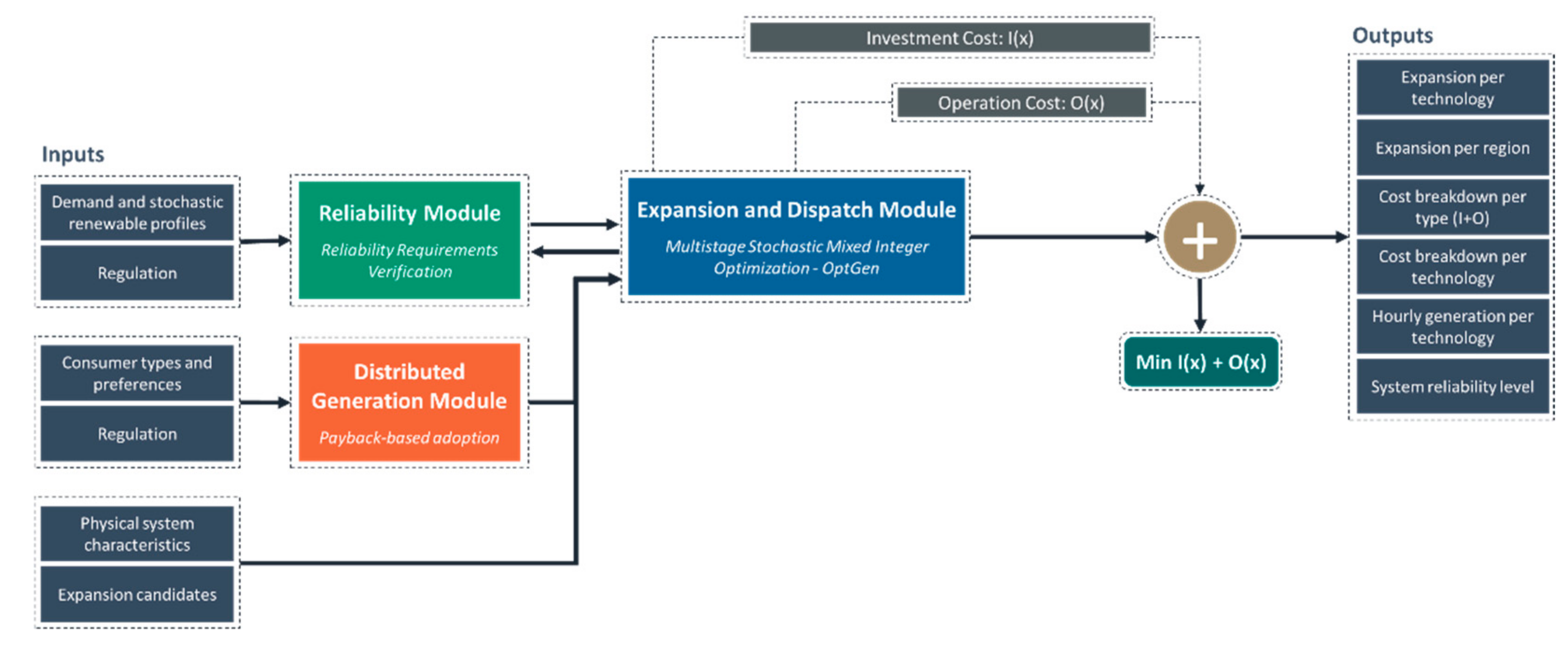
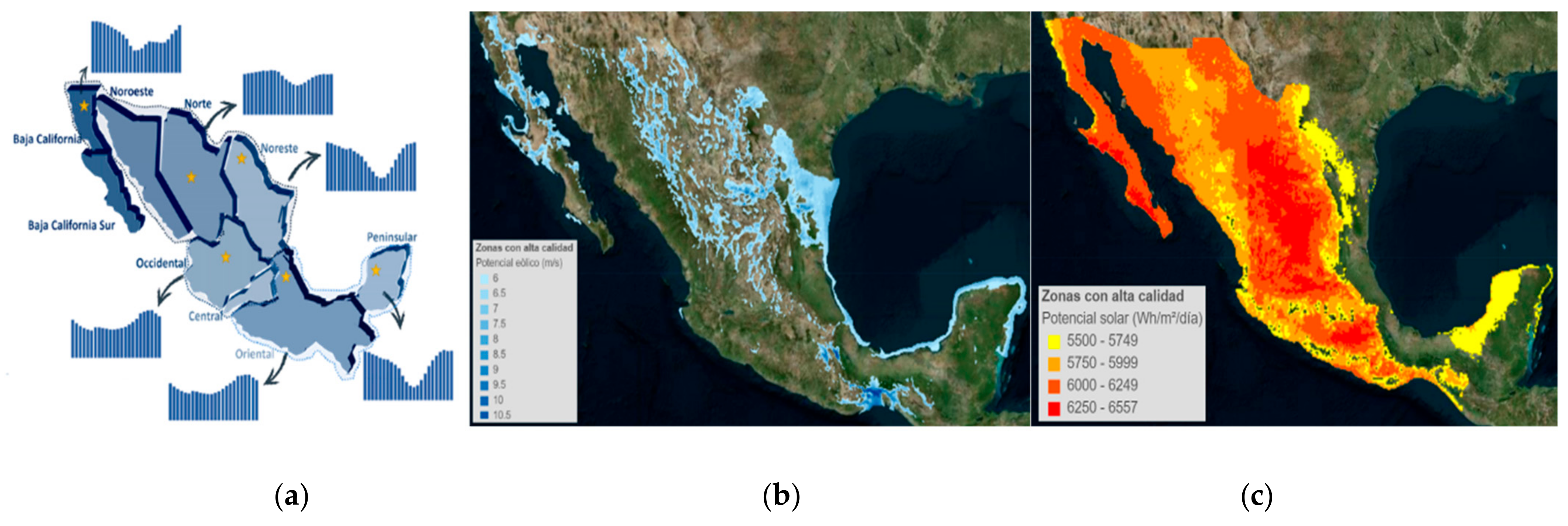
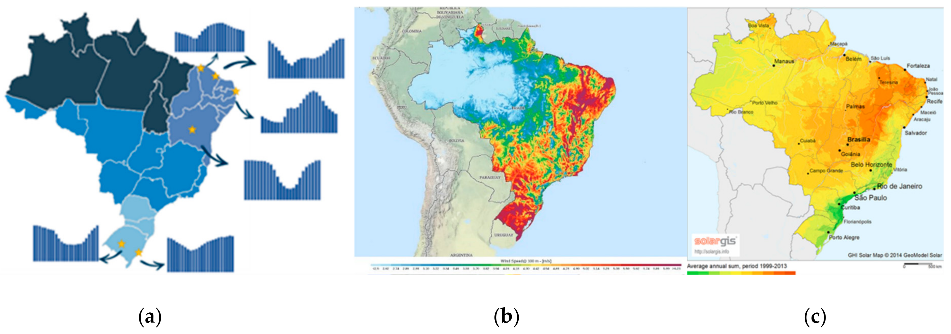


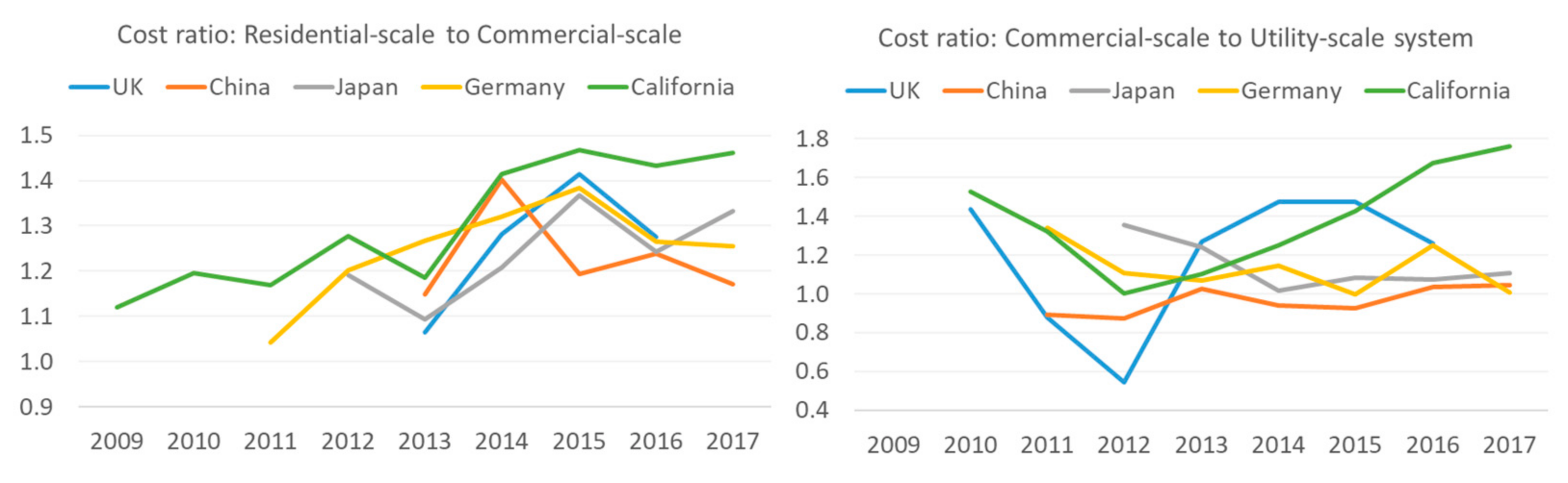


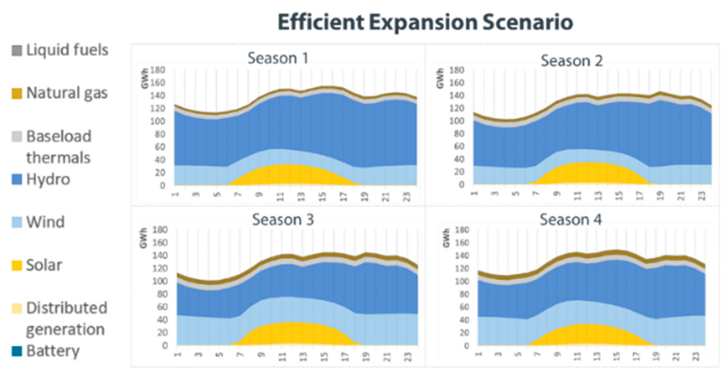
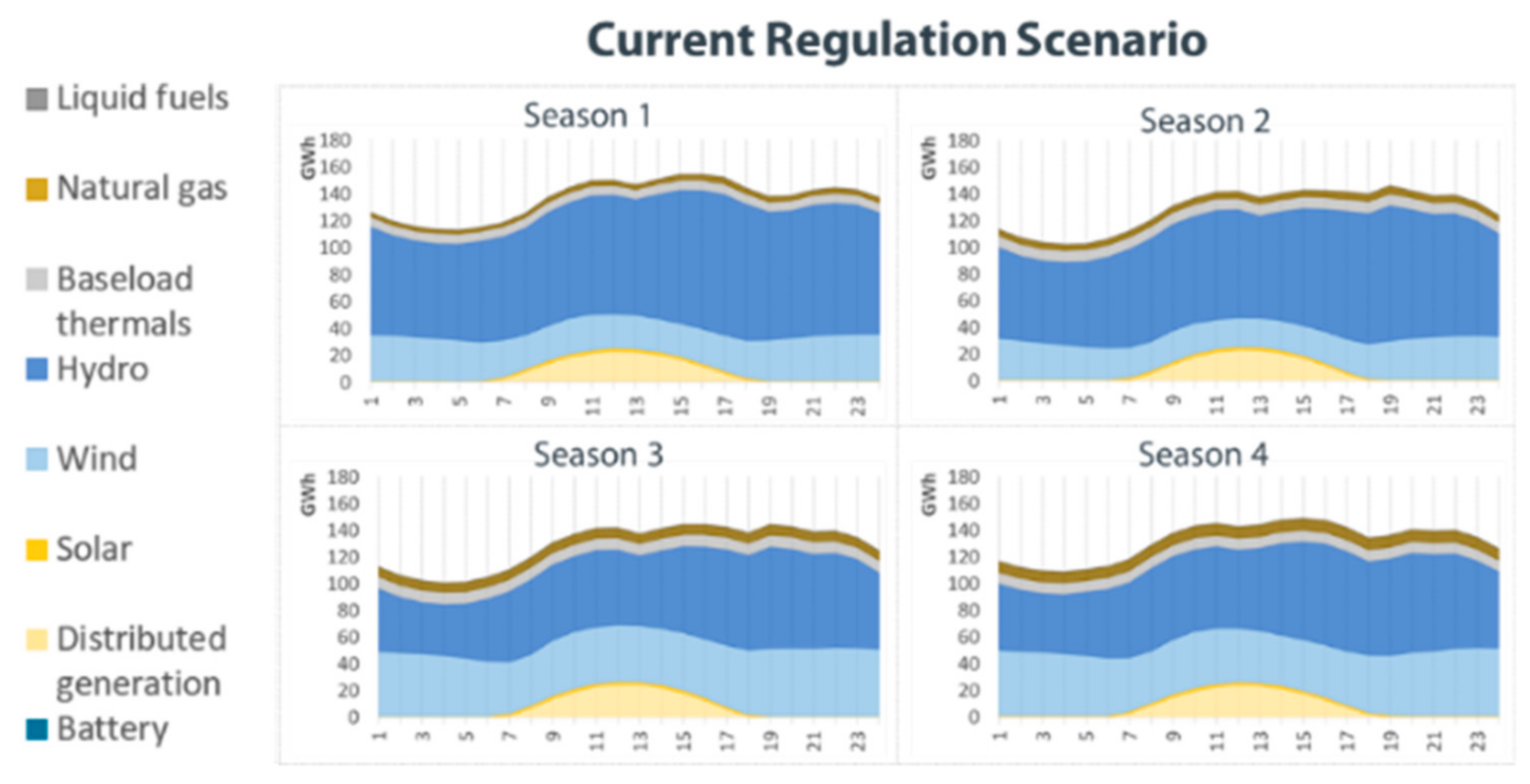

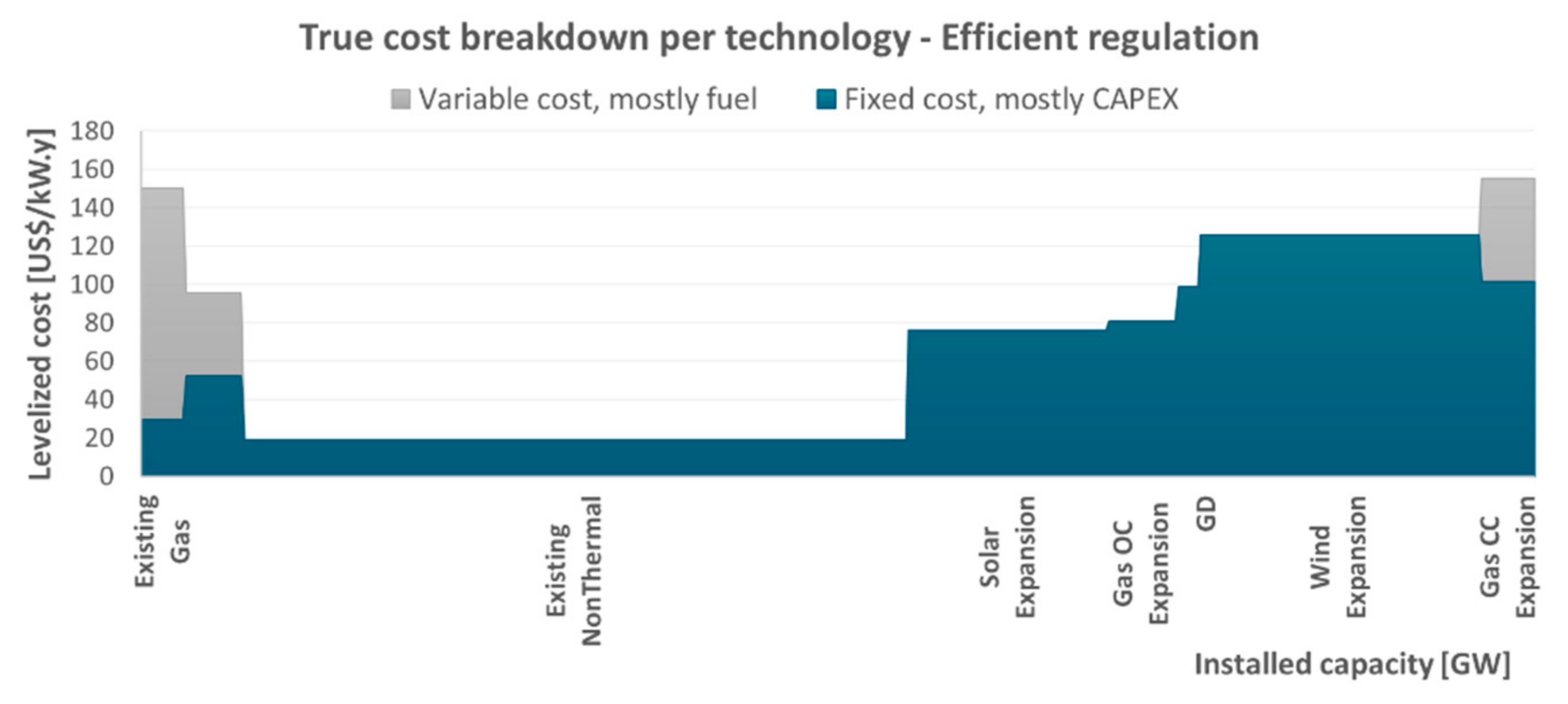


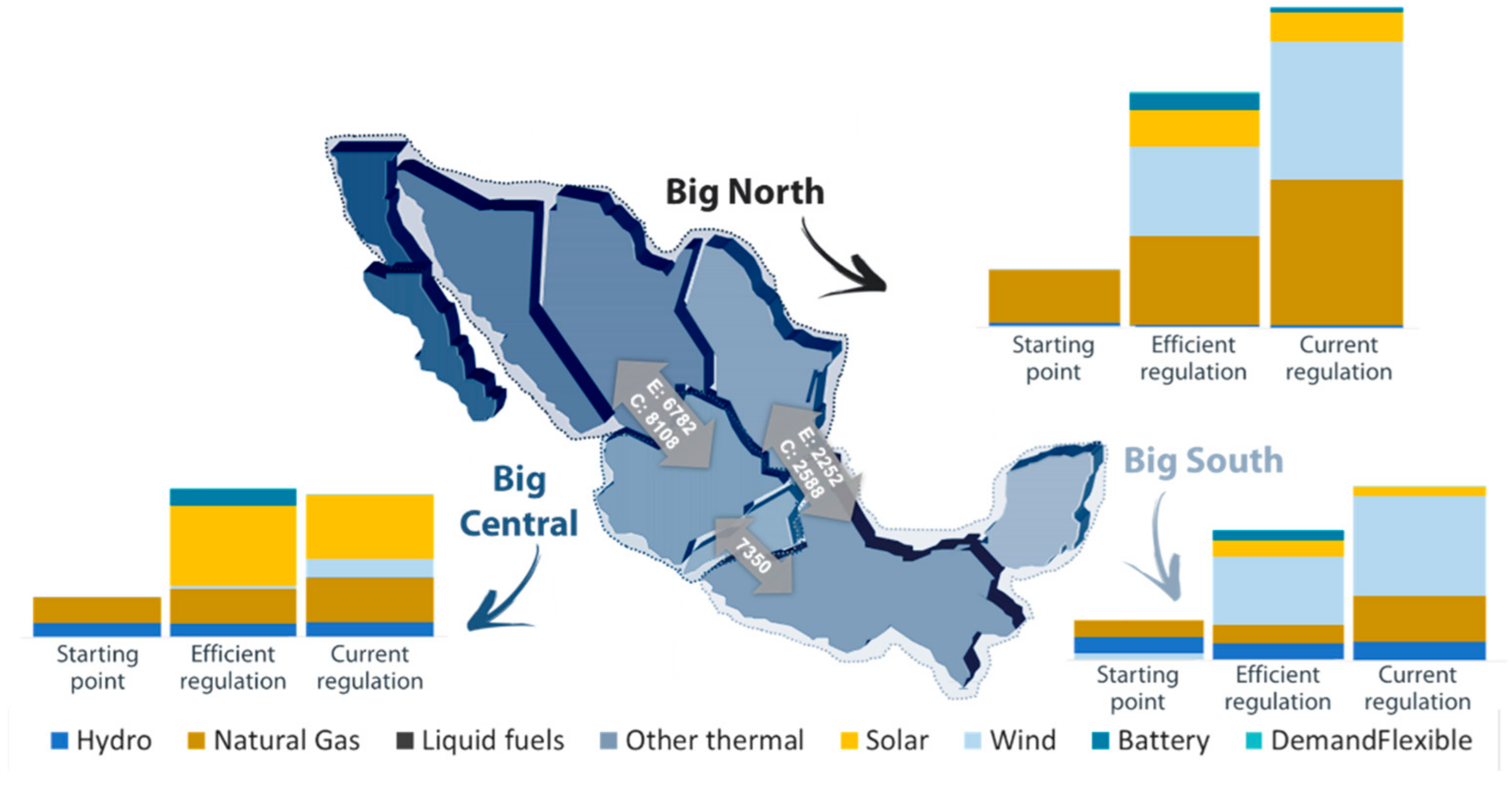
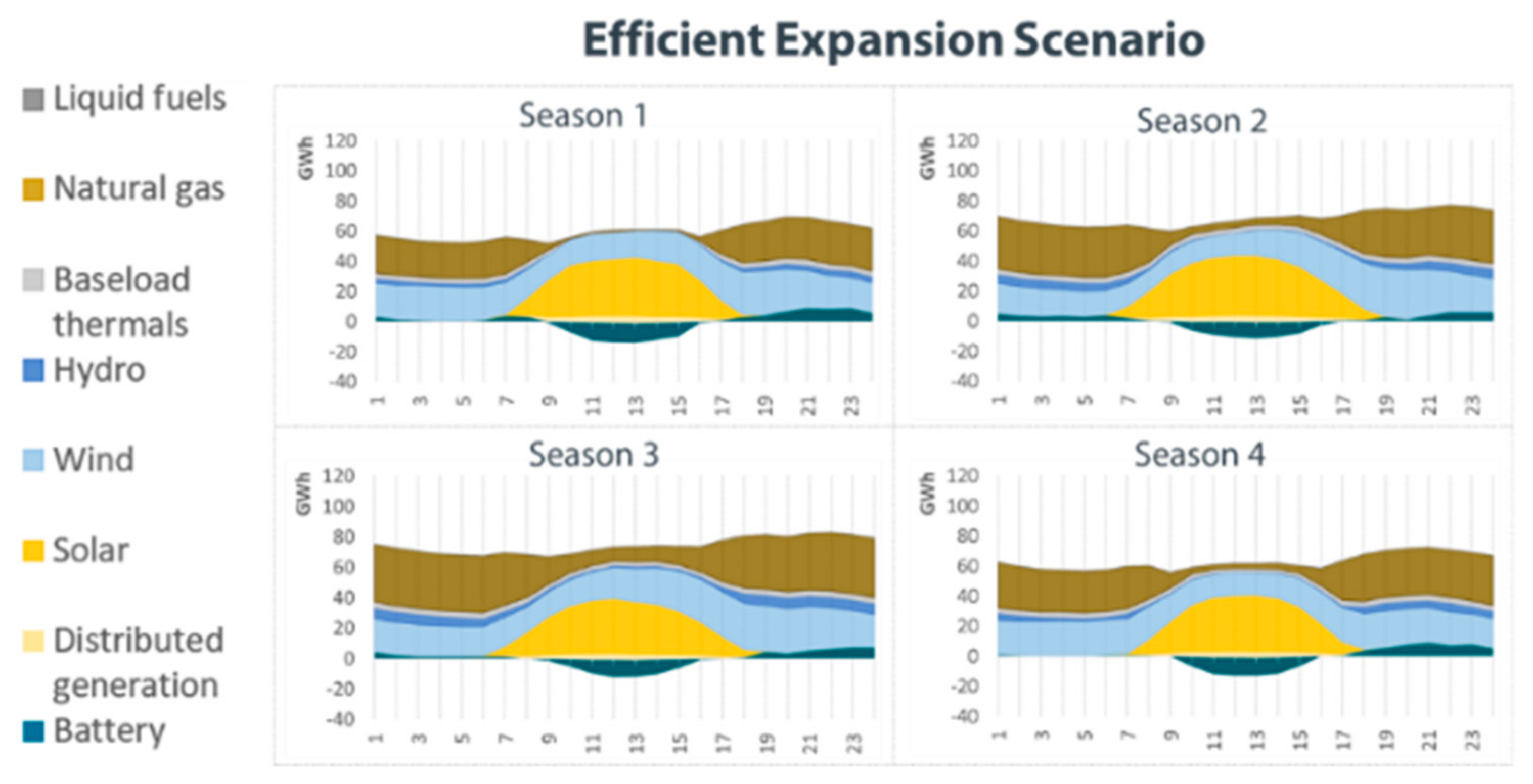


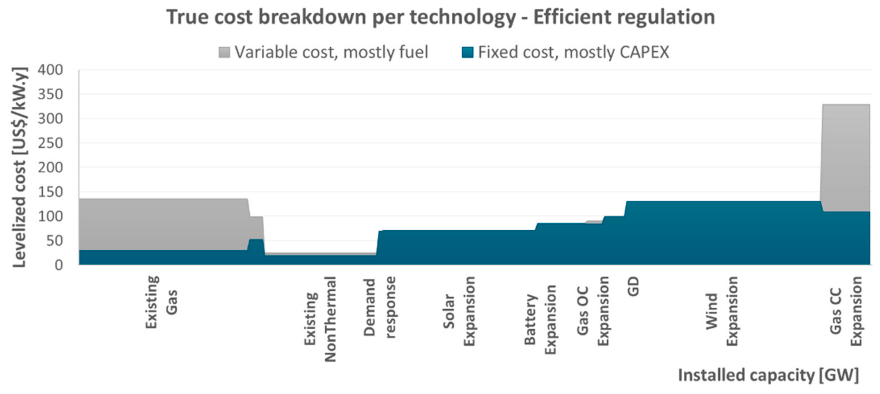
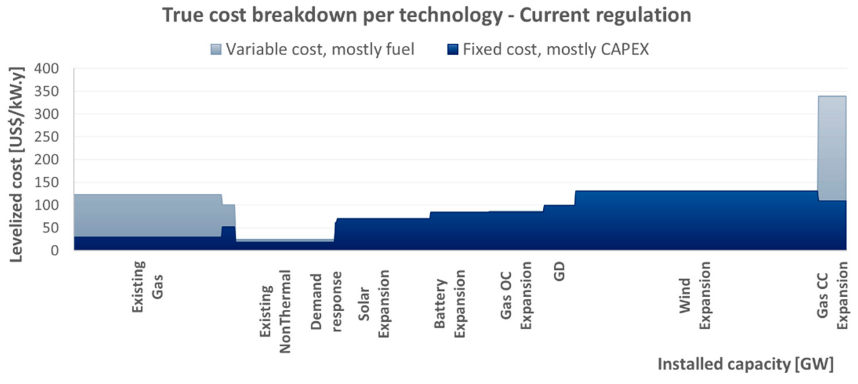
Publisher’s Note: MDPI stays neutral with regard to jurisdictional claims in published maps and institutional affiliations. |
© 2021 by the authors. Licensee MDPI, Basel, Switzerland. This article is an open access article distributed under the terms and conditions of the Creative Commons Attribution (CC BY) license (https://creativecommons.org/licenses/by/4.0/).