
Parameterized Trajectory Optimization and Tracking Control of High Altitude Parafoil Generation


Abstract
:1. Introduction
2. Parafoil Model and Problem Formulation
2.1. Model Establishment
- The parafoil and the cable gravity is:
- 2.
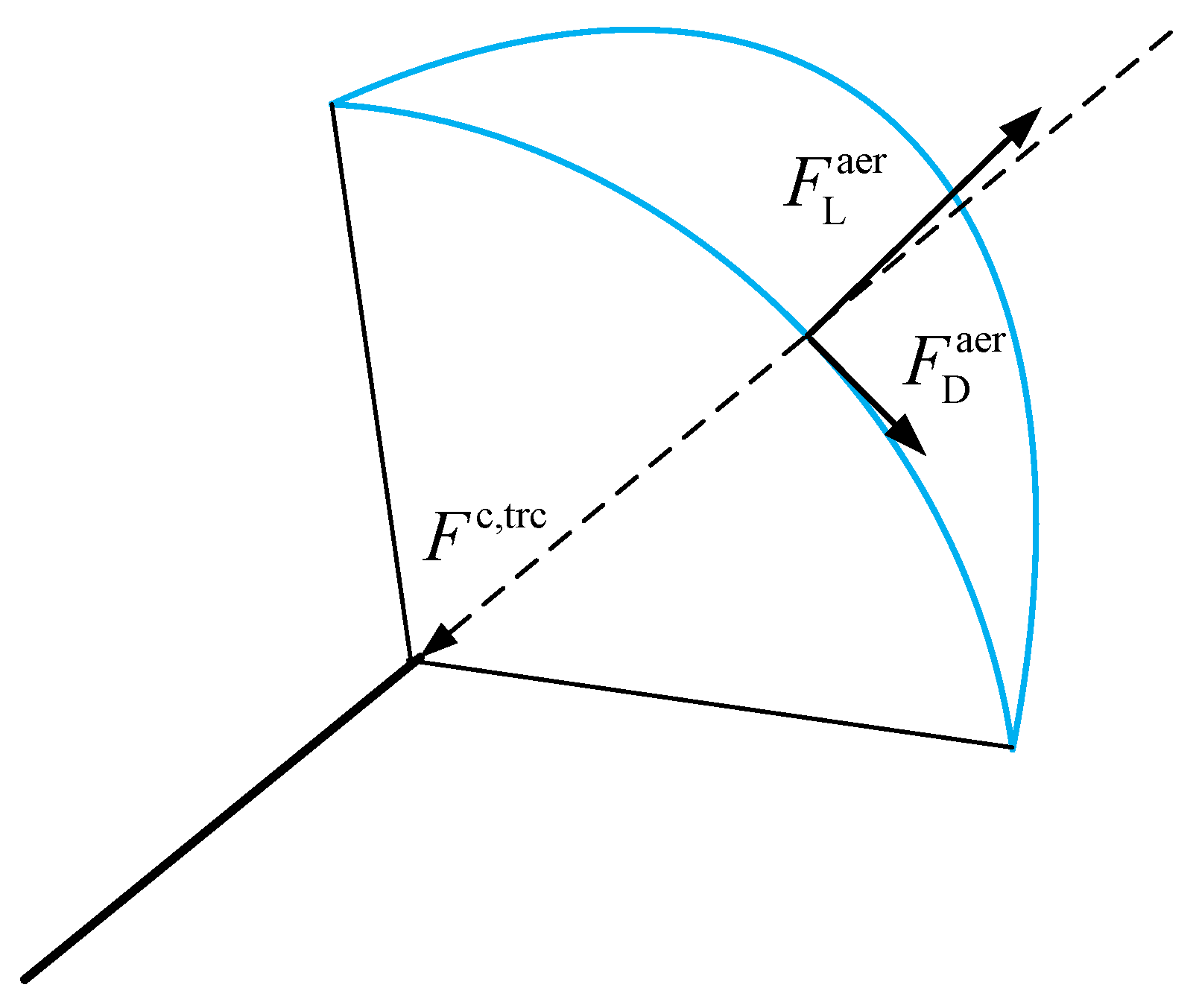
- The parafoil aerodynamic force (the forces acting on the parafoil in motion relative to the air, which includes aerodynamic lift and aerodynamic drag is:
- 3.
- The cable aerodynamic resistance is:
- 4.
- Apparent forces.
- 5.
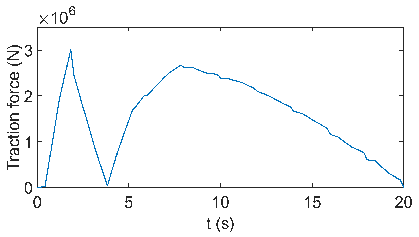
- The cable traction force is shown in Figure 4:
2.2. Problem Formulation
2.3. OCP Formulation
3. Parameterized Trajectory Optimization
- Time domain conversion:
- 2.
- Calculation of the distribution nodes:
- 3.
- State and control variables parameterization:
- 4.
- Elimination of the dynamic equations.
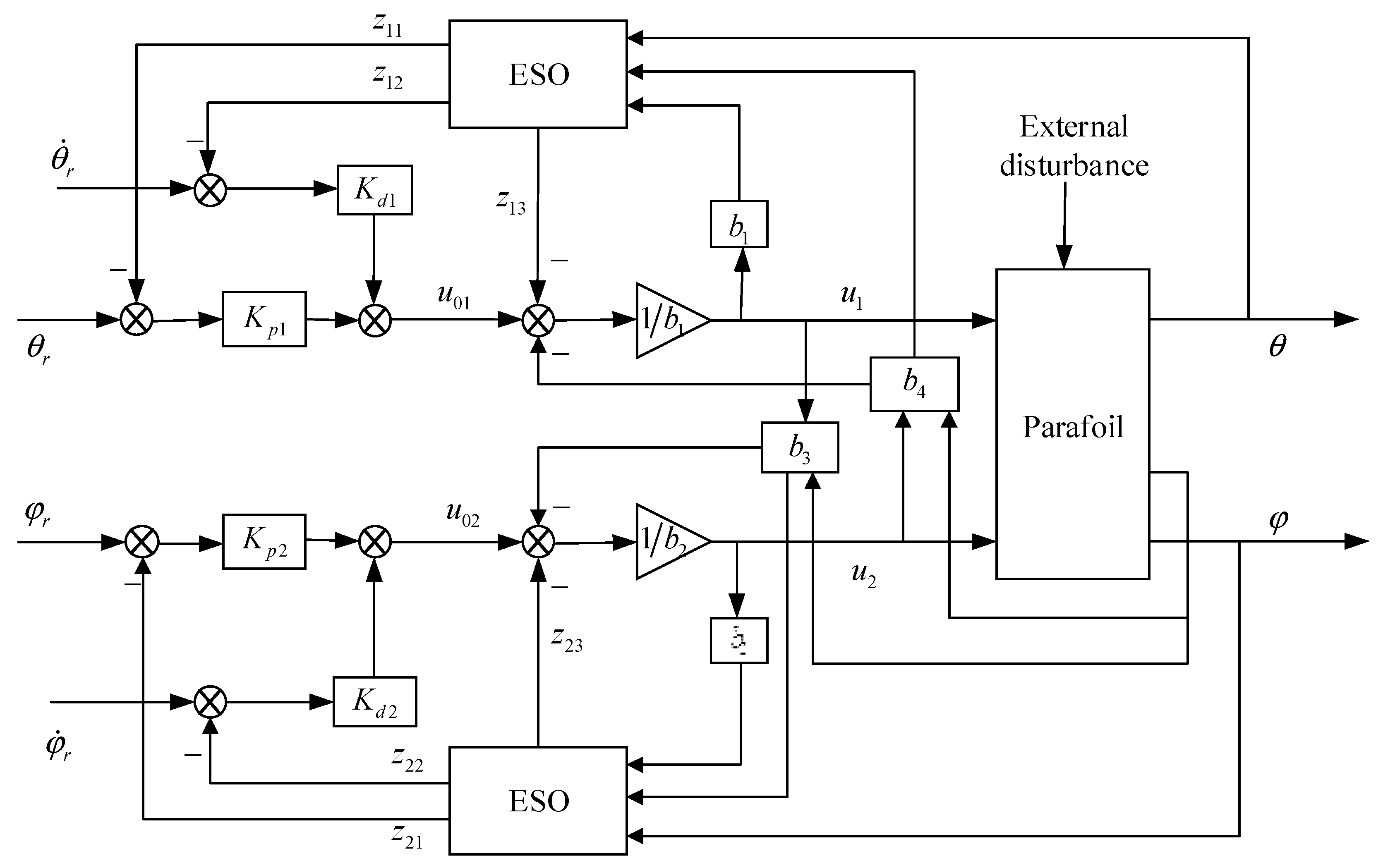
4. Trajectory Tracking Control
5. Optimization and Simulation Results
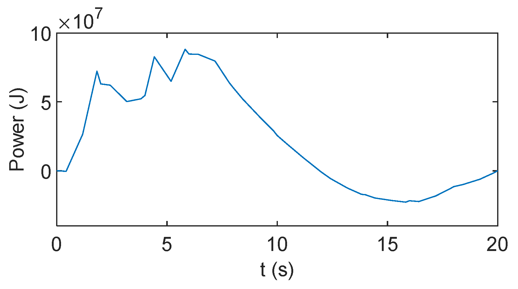
5.1. Optimization Results
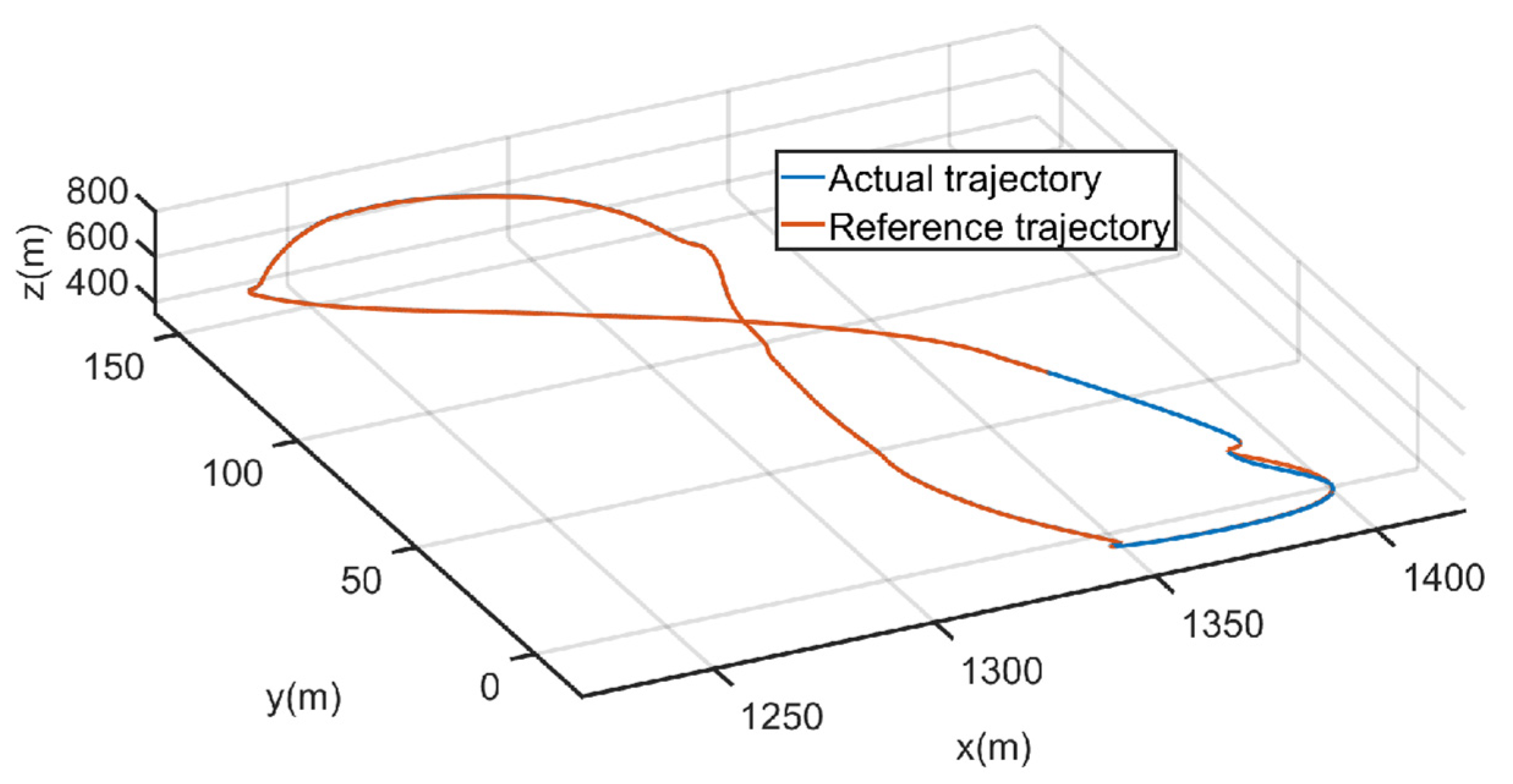
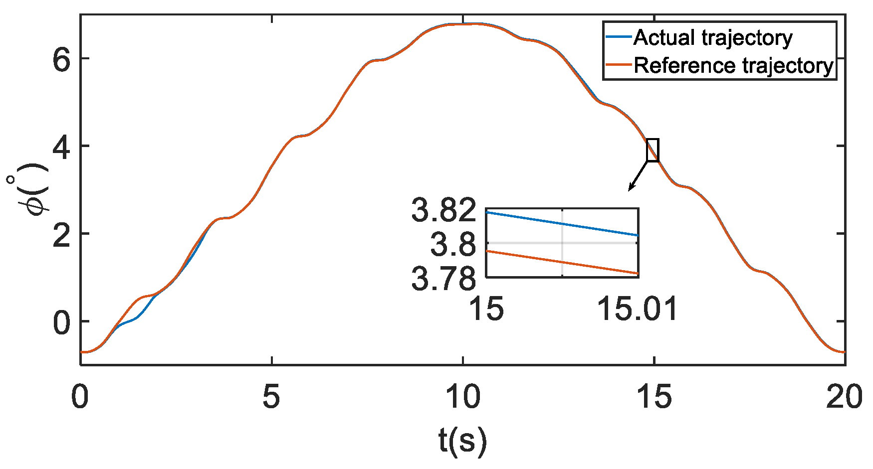
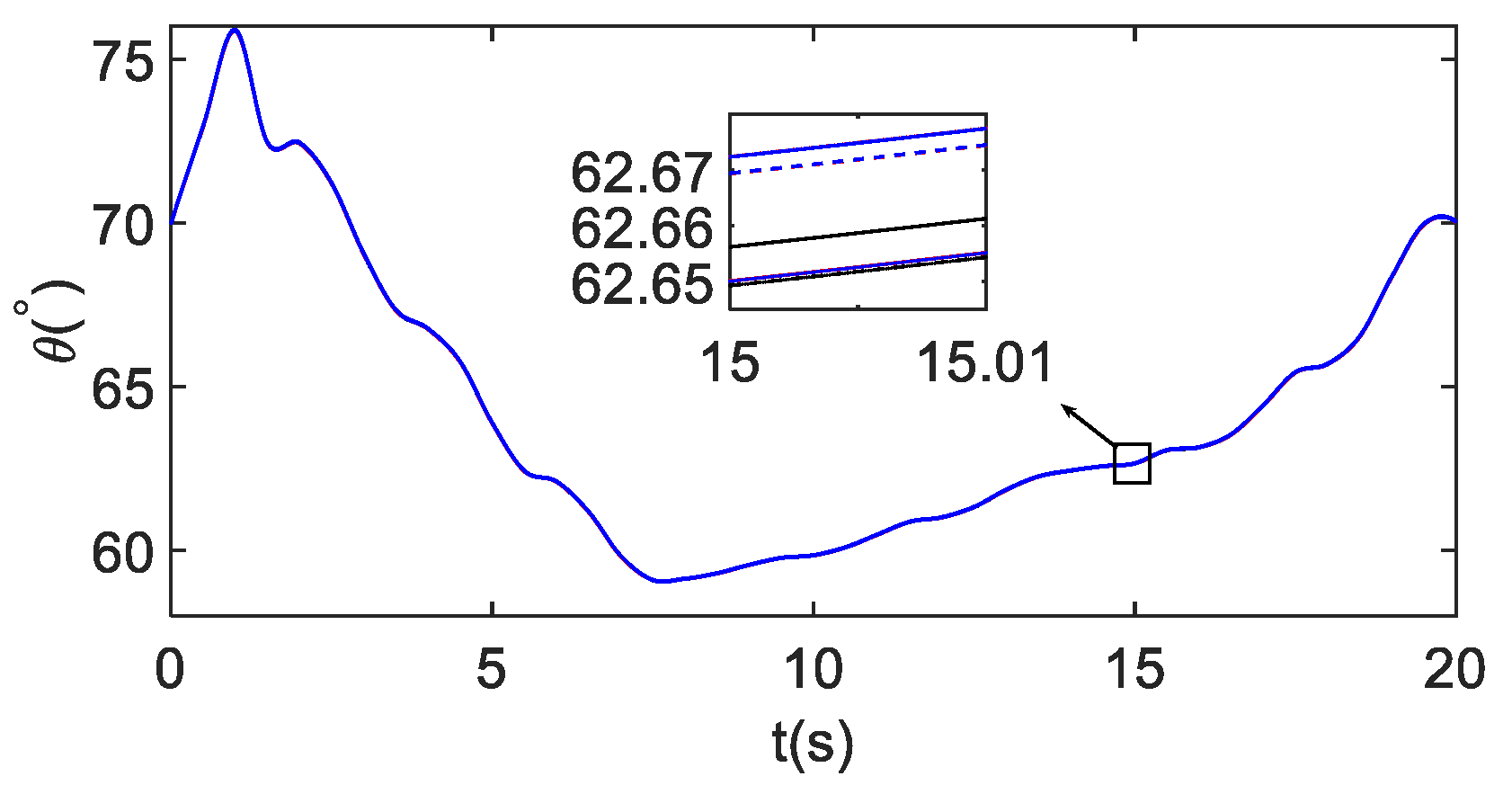
5.2. Tracking Control Results
5.3. Perturbed Cases and Monte Carlo Simulation
6. Conclusions
Author Contributions
Funding
Institutional Review Board Statement
Informed Consent Statement
Data Availability Statement
Conflicts of Interest
References
- Cao, Y.; Hu, Q.; Shi, H.; Zhang, Y. Prediction of wind power generation base on neural network in consideration of the fault time. IEEE Trans. Electr. Electron. Eng. 2019, 14, 670–679. [Google Scholar] [CrossRef]
- Archer, C.L.; Caldeira, K. Global assessment of high-altitude wind power. Energies 2009, 2, 307–319. [Google Scholar] [CrossRef] [Green Version]
- Mondal, A.K.; Mondal, S.; Devalla, V.; Sharma, P.; Gupta, M.K. Advances in floating aerogenerators: Present status and future. Int. J. Precis. Eng. Manuf. 2016, 17, 1–12. [Google Scholar] [CrossRef]
- Kim, J.; Park, C. Wind power generation with a parawing on ships, a proposal. Energy 2009, 35, 336–342. [Google Scholar]
- Ran, X.L. Study of Dynamics and Control on High Altitude Wind Power Generation Towing Parafoil; National University of Defense Technology: Changsha, China, 2012. [Google Scholar]
- Liu, Y.G.; Wang, Y.K.; Wan, Z.Q.; Yan, D. Research progress and prospect of tethered floating wind energy generation technology. Adv. Aeronaut. Sci. Eng. 2021, 12, 36–43. [Google Scholar]
- Cherubini, A.; Papini, A.; Vertechy, R.; Fontana, M. Airborne wind energy systems: A review of the technologies. Renew. Sustain. Energy Rev. 2015, 15, 1461–1476. [Google Scholar] [CrossRef] [Green Version]
- Costello, S. Real-Time Optimization via Directional Modifier Adaptation, with Application to Kite Control. Ph.D. Dissertation, EPFL, Lausanne, Switzerland, 2015. [Google Scholar]
- Loyd, M.L. Crosswind kite power. J. Energy 1980, 4, 106–111. [Google Scholar] [CrossRef]
- Zgraggen, A.U.; Fagiano, L.; Morari, M. On real-time optimization of airborne wind energy generators. In Proceedings of the 52nd IEEE Conference on Decision and Control (CDC), Florence, Italy, 10–13 December 2013; pp. 385–390. [Google Scholar]
- Zgraggen, U.; Fagiano, L.; Morari, M. Real-time optimization and adaptation of the crosswind flight of tethered wings for airborne wind energy. IEEE Trans. Control Syst. Technol. 2015, 23, 434–448. [Google Scholar] [CrossRef] [Green Version]
- Williams, P.; Lansdorp, B.; Ockesl, W. Optimal crosswind towing and power generation with tethered kites. J. Guid. Control Dyn. 2008, 31, 81–93. [Google Scholar] [CrossRef]
- Ilzhofer, A.; Houska, B.; Diehl, M. Nonlinear MPC of kites under varying wind conditions for a new class of large-scale wind power generators. Int. J. Robust Nonlinear Control 2007, 17, 1590–1599. [Google Scholar] [CrossRef]
- Canale, M.; Fagiano, L.; Milanese, M. High altitude wind energy generation using controlled power kites. IEEE Trans. Control Syst. Technol. 2010, 18, 279–293. [Google Scholar] [CrossRef]
- Song, J.; Zhao, K.; Weng, H.; Huang, X.; Liu, Y. Research on reliable path planning of manipulator based on artificial beacons. In Proceedings of the 2019 IEEE International Conference on Dependable, Autonomic and Secure Computing, International Conference on Pervasive Intelligence and Computing, International Conference on Cloud and Big Data Computing, International Conference on Cyber Science and Technology Congress, Fukuoka, Japan, 5–8 August 2019. [Google Scholar]
- Elnagar, G.; Kazemi, M.A.; Razzaghi, M. The pseudospectral Legendre method for discretizing optimal control problems. IEEE Trans. Autom. Control 1995, 40, 1793–1796. [Google Scholar] [CrossRef]
- Gong, Q.; Fahroo, F.; Ross, I.M. Spectral algorithm for pseudospectral methods in optimal control. J. Guid. Control Dyn. 2008, 31, 460–471. [Google Scholar] [CrossRef] [Green Version]
- Hu, W.J.; Lu, Q.; Chang, J. A Gauss pseudospectral method for reentry trajectory planning with characteristic trend partitioning. Acta Aeronaut. Astronaut. Sin. 2015, 36, 3338–3348. [Google Scholar]
- Chen, H.; Fang, Y.C.; Sun, N.; Qian, Y.Z. Pseudospectral method based on time optimal anti-swing trajectory planning for double pendulum crane systems. Acta Autom. Sin. 2016, 42, 153–160. [Google Scholar]
- Zhang, Y.B.; Zong, Q.; Lu, H.C. Formation trajectory optimization of quadrotor UAV based on HP adaptive pseudospectral method. Sci. China Technol. Sci. 2017, 3, 239–248. [Google Scholar]
- Erhard, M.; Strauch, H. Control of towing kites for seagoing vessels. IEEE Trans. Control Syst. Technol. 2013, 21, 1629–1640. [Google Scholar] [CrossRef] [Green Version]
- Fagiano, L.; Zgraggen Morari, M.; Khammash, M. Automatic crosswind flight of tethered wings for airborne wind energy: Modeling, control design, and experimental results. IEEE Trans. Control Syst. Technol. 2014, 22, 1433–1447. [Google Scholar]
- Li, H.; Olinger, D.J.; Demetriou, M.A. Attitude tracking control of an airborne wind energy system. In Proceedings of the 2015 European Control Conference (ECC), London, UK, 11–14 July 2015; pp. 1510–1515. [Google Scholar]
- Jiang, B.P.; Hamid, R.K.; Yang, S.C.; Gao, C.C.; Kao, Y.G. Observer-based adaptive sliding mode control for nonlinear stochastic Markov jump systems via T-S fuzzy modeling: Applications to robot arm model. IEEE Trans. Ind. Electron. 2020, 99, 1. [Google Scholar] [CrossRef]
- Han, J.Q. From PID to active disturbance rejection control. IEEE Trans. Ind. Electron. 2009, 56, 900–906. [Google Scholar] [CrossRef]
- Gao, Z.Q. Scaling and bandwidth-parameterization based controller tuning. In Proceedings of the American Control Conference, Denver, CO, USA, 4–6 June 2003; pp. 4989–4996. [Google Scholar]
- Huang, Y.; Xue, W.C. Active disturbance rejection control: Methodology and theoretical analysis. ISA Trans. 2014, 53, 963–976. [Google Scholar] [CrossRef] [PubMed]
- International Towing Tank Conference: ITTC Symbols and Terminology List Version 2014, September 2014. Available online: http://ittc.info/media/4004/structured-list2014.pdf (accessed on 16 May 2021).


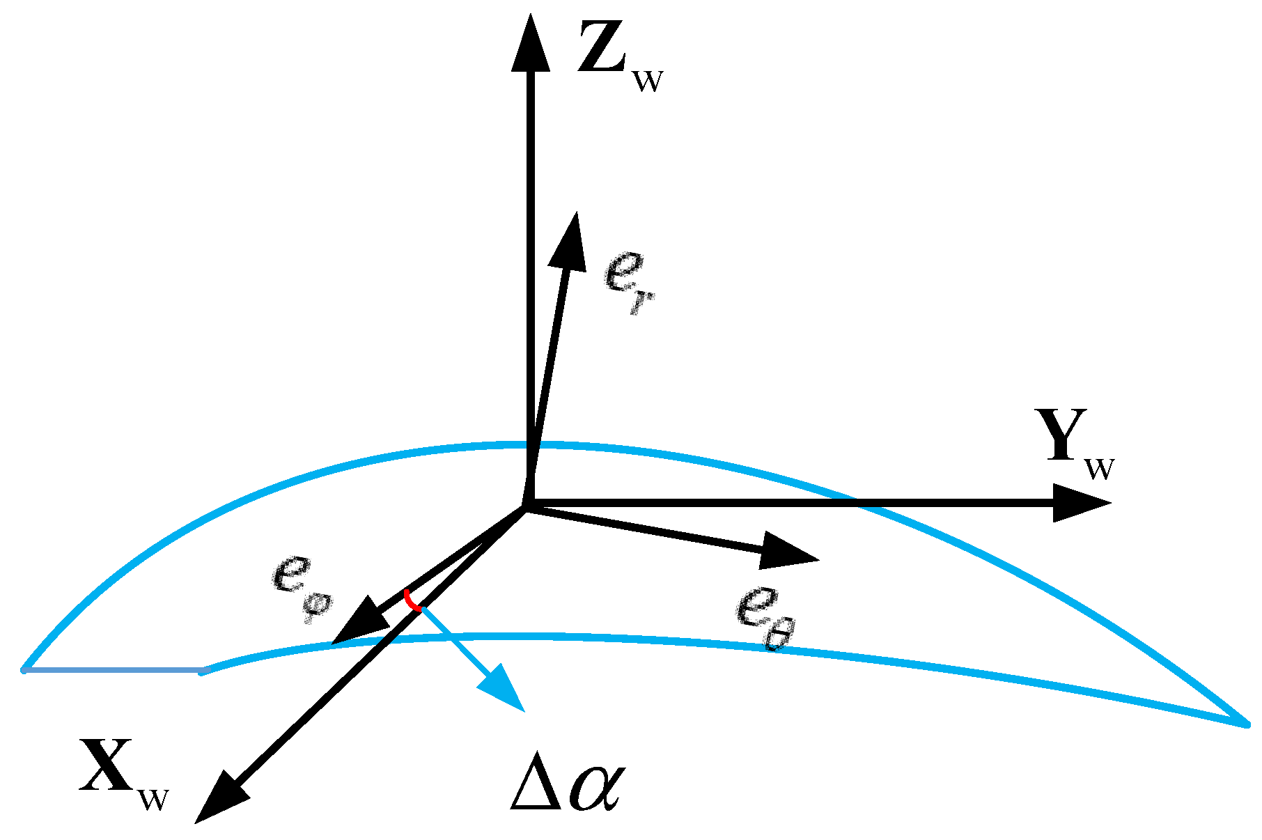
| Spherical coordinate in Figure 1. | ||
| Spherical coordinate in Figure 1. | ||
| Cable length in Figure 1. | ||
| Cable changing rate | ||
| Cable acceleration | ||
| Coordinate axis in Figure 1. | ||
| Coordinate axis in Figure 1. | ||
| Coordinate axis in Figure 1. | ||
| Parafoil area | ||
| Area of the line on the effective wind | ||
| Parafoil mass | ||
| Air density | ||
| Cable density | ||
| Cable diameter | ||
| Parafoil actual height | ||
| Reference altitude | ||
| Reference wind velocity | ||
| Parafoil coefficient of lift | ||
| Parafoil coefficient of drag | ||
| Cable coefficient of drag | ||
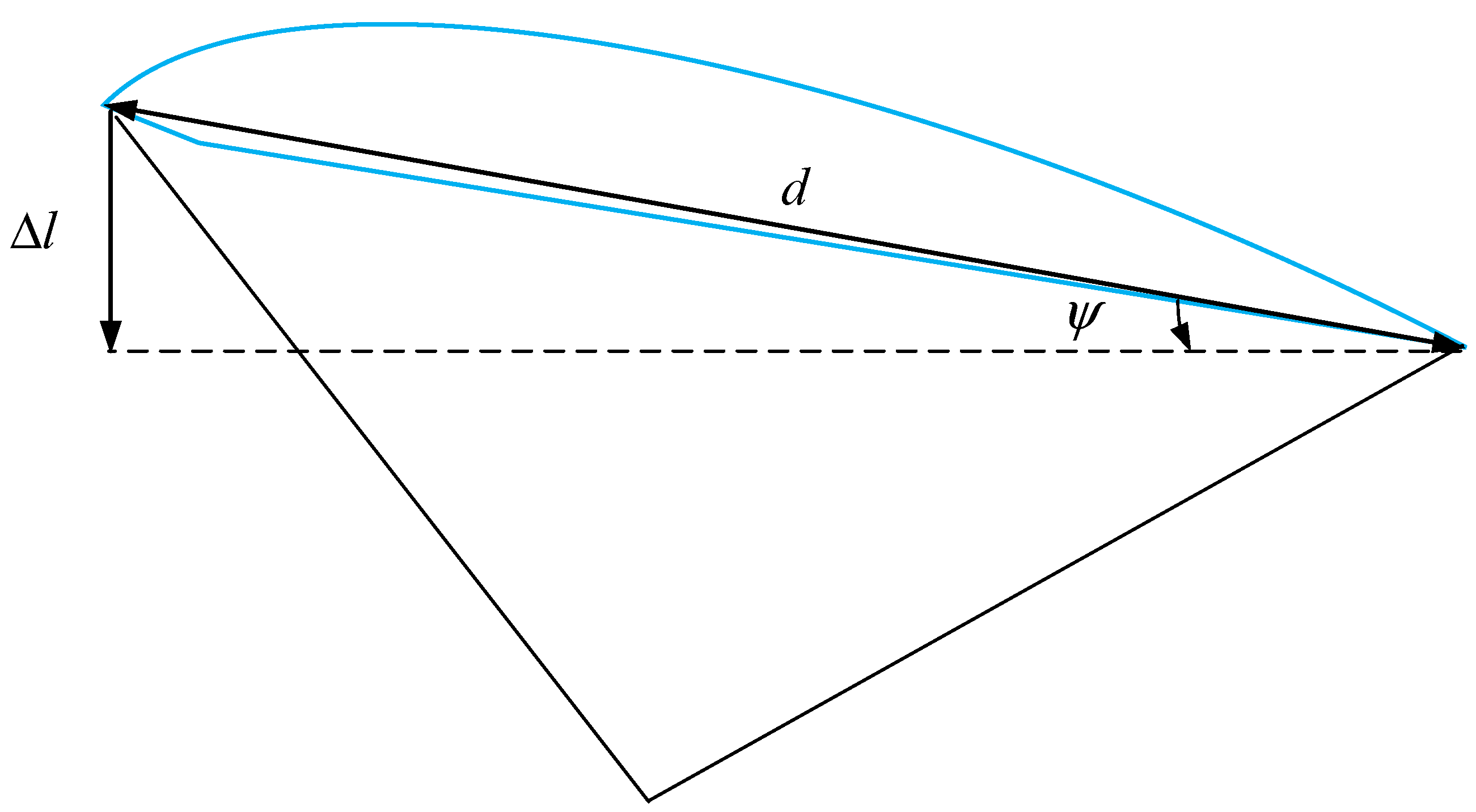
| Cable length difference at the two ends of the traction parafoil in Figure 2. | ||
| Length of the wingspan in Figure 2. | ||
| in Figure 2. | ||
| Angle between the effective wind velocity and the plane | ||
| Effective wind speed | ||
| Projection and unit vector of the effective wind speed on the plane | ||
| Wind coordinate axis | ||
| Wind coordinate axis | ||
| Wind coordinate axis | ||
| Parafoil and cable weight | ||
| Parafoil aerodynamic force | ||
| Cable aerodynamic force | ||
| Apparent force | ||
| Cable traction force | ||
| Aerodynamic lift force | ||
| Aerodynamic drag force |
| 850 | Kite mass | |
| 500 | Characteristic area | |
| 1.23 | Air density | |
| 970 | Line density | |
| 0.056 | Line diameter | |
| 1 | Line drag coefficient | |
| 100 | Reference altitude | |
| 10 | Reference wind velocity | |
| 9.81 | Gravity acceleration |
| Constraint Condition | Constraints | Range of the Constraints |
|---|---|---|
| State constraints | ||
| Control constraints | ||
| Control Parameters | Pitch Angle Channel | Yaw Angle Channel |
|---|---|---|
| 4 | 10 | |
| 15 | 12 | |
| 2.9 | 9 | |
| −11 | 13 |
| 8.82 | 0.00 | |
| 7.27 | 17.52 | |
| 10.7 | −21.28 | |
| 8.52 | 3.42 | |
| 9.84 | −11.54 | |
| 4.34 | 50.81 | |
| 8.02 | 9.06 | |
| 12.22 | −38.39 | |
| 7.67 | 13.05 |
Publisher’s Note: MDPI stays neutral with regard to jurisdictional claims in published maps and institutional affiliations. |
© 2021 by the authors. Licensee MDPI, Basel, Switzerland. This article is an open access article distributed under the terms and conditions of the Creative Commons Attribution (CC BY) license (https://creativecommons.org/licenses/by/4.0/).
Share and Cite
Long, X.; Sun, M.; Piao, M.; Chen, Z. Parameterized Trajectory Optimization and Tracking Control of High Altitude Parafoil Generation. Energies 2021, 14, 7460. https://doi.org/10.3390/en14227460
Long X, Sun M, Piao M, Chen Z. Parameterized Trajectory Optimization and Tracking Control of High Altitude Parafoil Generation. Energies. 2021; 14(22):7460. https://doi.org/10.3390/en14227460
Chicago/Turabian StyleLong, Xinyu, Mingwei Sun, Minnan Piao, and Zengqiang Chen. 2021. "Parameterized Trajectory Optimization and Tracking Control of High Altitude Parafoil Generation" Energies 14, no. 22: 7460. https://doi.org/10.3390/en14227460