Article

Study on Optimum IUPAC Adsorption Isotherm Models Employing Sensitivity of Parameters for Rigorous Adsorption System Performance Evaluation

1
International Institute for Carbon-Neutral Energy Research (WPI-I2CNER), Kyushu University, 744 Motooka, Nishi-ku, Fukuoka 819-0395, Japan
2
Department of Statistics, University of Dhaka, Dhaka 1000, Bangladesh
3
Department of Nuclear Engineering, University of Dhaka, Dhaka 1000, Bangladesh
4
Institute for Materials Chemistry and Engineering, Kyushu University, Kasuga-koen 6-1, Kasuga-shi 816-8580, Japan
5
Department of Electronics and Telecommunication Engineering, Bangabandhu Sheikh Mujibur Rahman Science & Technology University, Gopalganj 8100, Bangladesh
6
Mechanical Engineering Department, Kyushu University, 744 Motooka, Nishi-ku, Fukuoka 819-0395, Japan
*
Author to whom correspondence should be addressed.
Energies 2021, 14(22), 7478; https://doi.org/10.3390/en14227478
Submission received: 15 September 2021 / Revised: 19 October 2021 / Accepted: 1 November 2021 / Published: 9 November 2021
(This article belongs to the Special Issue Alternative and Emerging Cooling and Heating Technologies)

Abstract

:
Adsorption cooling technologies driven by low-grade thermal or solar power are used as an energy-efficient alternative to conventional refrigeration and air conditioning systems. Explicit understanding of the adsorption cycles requires precise determination of the performance parameters, replication of the experimental data, and the rigorous study of the adsorption heat transformation method. Hence, the optimum adsorption isotherms model must be identified. Scientists often face difficulties in selecting the suitable isotherm model as there are many models for a particular form of adsorption isotherm. The present study introduces a novel approach for choosing the optimal models for each type of International Union of Pure and Applied Chemistry (IUPAC) classified adsorption isotherm using robust statistical methods. First, the box-and-whisker plots of error identification are employed. Tóth for Type-I(a) and Type-I(b), modified BET for Type-II, GAB for Type-III, Universal for Type-IV(a), and Type-IV(b), Sun Chakrabarty for Type-V, and Yahia et al. for Type-VI were found lower than the other candidate models in box-and-whisker plot. The optimality of our selected models was further verified using analysis of variance (ANOVA), pairwise Tukey honest significant difference (HSD) test, Kruskal–Wallis rank-sum test, and pairwise Wilcoxon rank-sum test. In short, rigorous statistical analysis was performed to identify the best model for each type of isotherm by minimizing error. Moreover, specific cooling effect (SCE) of Maxsorb III/ethanol and silica gel/water pairs were determined. Results showed that Tóth is the optimal isotherm model for the studied pairs, and the SCE values obtained from the model agree well with experimental data. The optimum isotherm model is indispensable for the precise designing of the next generation adsorption cooling cycles.

1. Introduction

Thermally driven cooling technologies are receiving a lot of interest from scientists as a way to minimize world electricity demand. Adsorption-based cooling systems, which can be powered by low-grade thermal energy, have been shown to be particularly successful in this regard. Waste heat [1,2,3] or heat from cost-effective no-concentrating solar thermal collectors [4,5,6,7] can be used for this reason. An adsorbent bed, a heat exchanger in which the adsorbent materials are kept, is one of the most important components of an adsorption refrigeration system. The beds go through adsorption and desorption activities in the adsorption cycles to produce thermal compression of the refrigerant vapor [8].
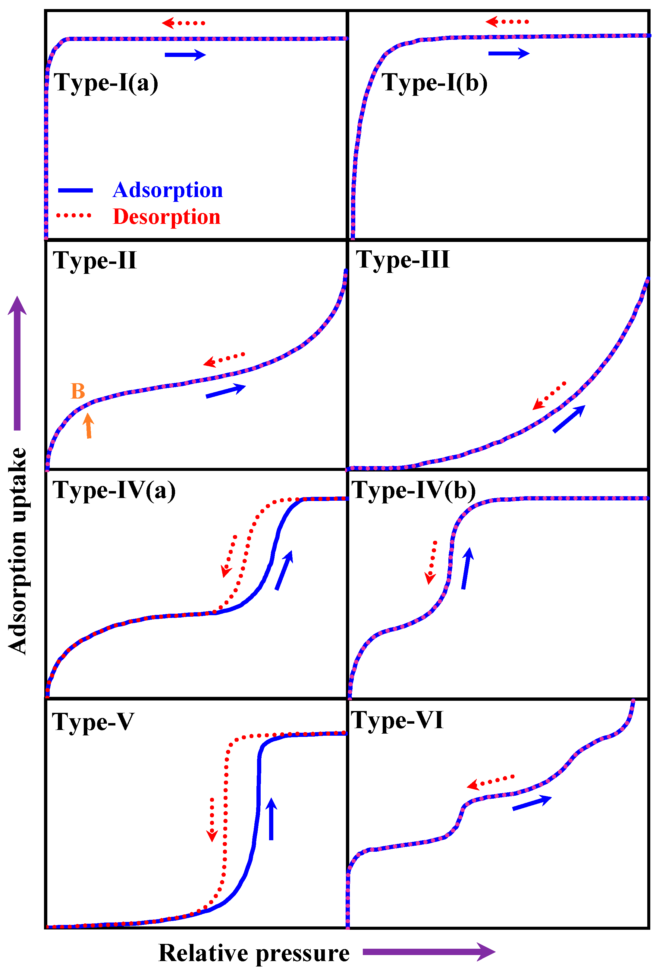
Adsorption/desorption isotherms are obtained at various adsorption temperatures by varying the pressure of the adsorbate. The highest amount of adsorbate which can be absorbed by the adsorbent at a given pressure is determined by these isotherms. Moreover, different adsorbent/adsorbate pairs show different isotherm shapes, and often a hysteresis is also observed. It is essential to relate experimental data from various adsorption pairs with different isotherm models in order to reproduce them. The International Union of Pure and Applied Chemistry (IUPAC) [9] defines adsorption isotherms into eight categories depending on their nature, as shown in Figure 1. In general, isotherm data are correlated using a variety of isotherm models, with the best-fitted model being used to examine adsorption characteristics. Rocky et al. [10] recently developed a zeolite-graphene composite for next-generation adsorption heat pump systems. They examined water adsorption onto these composites and used three isotherms to correlate the experimental data: modified Langmuir, Sun and Chakrabarty, and Universal model. Jahan et al. [11] used an energy-efficient, environmentally friendly, fast, and ultrasonication-assisted room temperature technique to synthesize MOF-801. For water adsorption onto MOF-801, the Sun and Chakrabarty, D-A, and Universal models were utilized. According to the literature, various pairs exhibit different adsorption isotherms, and multiple scholars have attempted to discover the best model for these types [12].
The optimum models for IUPAC classified isotherms were identified using a statistical approach [12]. The parameters of the models were determined by applying the generalized reduced gradient (GRG) technique. The GRG approach fits the candidate models by visualizing the fitted graph, which minimizes the root mean square error deviation (RMSD). However, the procedure relies on graphical tuning for optimum solutions. Thus, the results are subjective and often vary from one experimenter to another. Moreover, during optimization, if the estimate of a parameter deviates substantially, it may affect the results for the remaining parameters. Thus, the sensitivity or deviation in the parameter estimates should be considered while selecting the best model. The previous study [12] further applied the information-based criteria to identify the best model. The commonly used information criteria often select the complex model, i.e., the model which contains a relatively large number of parameters. Thus, the subjective choice of the parameter estimates in the GRG approach may affect the candidate models differently. This paper addresses these issues by considering simulation-based sensitivity analysis of the candidate models. Therefore, this study improves the previous work by examining the effect of random variation in the choice of estimates for the models.
A data set of adsorbent–adsorbate pairs is analyzed for each type of IUPAC classified isotherms in this study. Assuming that the estimated parameters [12] are close proximities to the actual values, the simulated estimates are obtained from the multivariate normal distribution for each candidate model. The current work aims to find the best isotherm models for all types of IUPAC classified isotherms, which was achieved by:
(i)
Examining the isotherm models and statistical methodologies.
(ii)
The model parameters have been optimized employing the generalized reduced gradient (GRG) non-linear optimization technique.
(iii)
The optimized parameters are varied deliberately within a small range of a large number (N = 10,000) of times to generate the empirical distributions of the RMSD.
(iv)
Box-and-whisker plots have been constructed of all candidate models for all types of IUPAC isotherms.
(v)
The parametric method ANOVA and Tukey HSD tests, as well as non-parametric method Kruskal–Wallis and Wilcoxon rank-sum tests, have been applied to find the significantly optimum models by minimizing RMSD.
(vi)
The robustness has been confirmed by determining the specific cooling effect (SCE) of Maxsorb III/ethanol and silica gel/water pairs.

2. Adsorption Isotherm Models

The adsorption isotherm model can explain the equilibrium uptake at a specific temperature for a certain adsorbent–adsorbate pair [13]. The researchers suggested various isotherm models to replicate the experimental data of different adsorption pairs. Table 1 presents the models considered in this study.

3. Error Evaluation Function

In this study, root mean square error deviation (RMSD) functions are adopted to optimize model parameters. Researchers often use this RMSD [21,40] error function, which can be expressed as:
RMSD = i = 1 n ( W e x p W c a l ) i 2 n
Here Wexp and Wcal represent experimental uptake and model uptake, respectively and n is the number of observations. RMSD error function can be used to determine model parameters that consider a large irregular error.

4. Simulation Approach

The parameters of the candidate models are estimated graphically using the GRG non-linear optimization technique in Excel. Thus, the best choice for the estimates is often subjective and may deviate with a measurement error in case different researchers analyze the same data or slightly different data are obtained even though the experiment is repeated under the same condition.
Since conducting experiments are time-consuming and highly expensive, it is not feasible to replicate the experiments many times and capture the variation in the estimates of model parameters. As a result, we cannot examine directly how the subjective choice or measurement error results in biased estimates of parameters. In other words, the effect of experimental variability on the variation of parameter estimates from the GRG approach cannot be assessed. Thus, the prediction of experimental outcomes by the different candidate models may be affected by the bias due to measurement error. This study examines the effect empirically, i.e., by adopting a simulation-based comparison of RSMD of the candidate models. The simulation approach randomly changes the estimates of model parameters proposed in [12] and is assumed to be reliable. For a given model, the deviation from the estimates θ ^ of [12] takes place deliberately by (i) generating random samples from a multivariate normal distribution with mean vector equals the vector of estimates θ ^ or (ii) adding to the estimates a randomly selected sample from N (0,1) as the measurement error terms for the GRG method.
Thus, the above procedure results from a set of RSMD for the candidate models attributed to the measurement error or bias due to subjective choice of parameter estimates from the graphs. We perform the simulation approach a large number of times and compare the prediction performance of the models based on the empirical distribution of RSMD.
Given a set of parameters θ = ( θ 1 , θ 2 , , θ p ) with the proposed estimates θ ^ = ( θ ^ 1 , θ ^ 2 , , θ ^ p ) , which are assumed to have minimum prediction error, the procedure (i) can be stated as follows.
(a)
Randomly select a vector from x = ( x 1 , x 2 , , x p ) from a multivariate normal distribution with mean vector θ ^ and variance–covariance matrix Σ . We assume that the variances are small (0.01, 0.001, etc.), i.e., the variability in the choice of estimates from the GRG graph is not substantial.
(b)
Obtain the predicted values of the experimental outcomes by using the selected estimates and compute the corresponding RMSD’s.
(c)
Repeat (a) and (b) a large number (10,000) of times and compare the prediction performance of the models based on the empirical distributions of the RSMD’s.
Unlike (i), (ii) assumes that the random (measurement) errors or bias terms follow a normal distribution. Thus, the procedure is different from (i) in that the simulated estimates in (a) are obtained by randomly generating a sample from N (0,1) and adding to θ ^ .
We adopt the simulation-based approaches and compare the results for each model in Table 1. Thus, the sensitivity of the models is examined under the condition where the parameter estimates are slightly biased due to the subjective judgment of the experimenters using the graphical GRG technique.

5. Statistical Tools

5.1. The Box-and-Whisker Plot

The box-and-whisker plot [41] is a chart comprising five concise statistics, which are the smallest (min), 1st quartile (Q1), 2nd quartile (Me), 3rd quartile (Q3), and the maximum (max) value of a data set. In this plot, a box is drawn from the first quartile (Q1) to the third quartile (Q3). Median (Me) is a perpendicular line that goes between Q1 and Q3. The whiskers are a line from Q1 to minimum and Q3 to the maximum. This plot divides the total number of observations into four groups, as shown in Figure 2.

5.2. Analysis of Variance (ANOVA)

The statistician Ronald Fisher developed ANOVA [41,42]. In ANOVA, the total variation in a data set is divided into different influential factors known as sources of variation. ANOVA provides a test for equality of several means (F-test), a generalization of t-test for more than two means. The null hypothesis is given by-
Hypothesis H0:
μ1 = μ2 = μ3 ... = μk vs.
Hypothesis H1:
At least two means are unequal.
Where k indicates the number of independent groups for comparison.
The test statistic is given by, F = M S B e t M S W i t h ; where, M S B e t = S S B e t K 1 and M S W i t h = S S W i t h N k . MSBet indicates between the mean sum of squares and MSWith measures within the mean sum of squares of the candidate models. N indicates the number of observations, and K defines the number of candidate models in each type.

5.3. Pairwise Test (Tukey’s HSD Test)

Tukey’s test (HSD test) [43] can be used to determine whether two means are significantly different or not. Dunnett’s and Scheffe’s tests are two further multiple comparison tests. We might compare the two group means using a t-test with only two different groups of observations. Because of the issue of multiple comparisons, it is incorrect to compare each pair using a t-test when there are more than two groups. The proper way to carry out the study is to employ a one-way ANOVA to see if there is any evidence that the population means differ. If the ANOVA reveals that the group means differ, we may want to look into which of the means is different. The Tukey HSD test is applied in this case. Tukey’s test is a multiple comparison test that can be used when comparing more than two means. Tukey’s HSD test is usually used after the ANOVA F-test to determine which pairs of means are substantially different. The HSD can be calculated using the following formula-
H S D = q M S n
MS stands for mean square value, n for the number of observations in each group, and the Studentized range distribution table provides the value for q. The information can be found in D.G. Altman’s book named “Practical Statistics for Medical Research” (1995) [44].

5.4. Non-Parametric Method

The population distribution or sample size are not specified in a non-parametric technique [45]. Most parametric approaches, on the other hand, assume quantitative data, a normal population, and a suitably high sample size. Non-parametric inferences are less powerful than parametric findings in general. However, non-parametric approaches are robust, flexible, and suitable to non-quantitative data since they make fewer assumptions. In this study, the non-parametric methods are considered to validate the results from parametric methods.

5.5. Kruskal–Wallis Rank-Sum Test

The generalization of a rank-sum test when the number of groups l ≥ 2 is known as the Kruskal–Wallis test [46]. It is also known as the Kruskal–Wallis H-test. Here, the normality assumption of the population like ANOVA is not considered. The null hypothesis of this test is-
Hypothesis H0:
All sample/groups come from the same population, vs.
Hypothesis H1:
They come from different populations.
The test statistic is- h = 12 n ( n + 1 ) i = 1 l r i 2 n i 3 ( n + 1 ) , here, ri is the sum of ranks of ith group, n = n 1 + n 2 + n 3 + + n l is the total number of observations, and h is distributed as chi-square distribution with (l-1) degrees of freedom.

5.6. Wilcoxon Rank-Sum Test with Continuity Correction

Wilcoxon rank-sum [47] test is appropriate for two samples t-test where the population distribution is not normal. The null hypothesis is H 0 : μ 1 = μ 2 against H 1 : μ 1 μ 2 or H 1 :   μ 1 μ 2 or H 1 : μ 1 μ 2 . The test statistic (normal approximation) is given by- N = n 1 + n 2   z = W n 1 ( N + 1 ) / 2 n 1 n 2 ( N + 1 ) / 12 is normally distributed with mean zero and variance one. Where N = n 1 + n 2 and W indicates the sum of ranks of the first sample.

6. Specific Cooling Effect

A significant performance parameter that can be measured using the equation below is the specific cooling effect (SCE) [24,48].
SCE = ( W max W min ) [ Δ h e v a T e T c C p r e f d t ]
Wmax indicates the maximum uptake, and Wmin means the minimum uptake. The enthalpy of vaporization is represented by ∆heva, and Cpref is the refrigerant specific heat. Wmax and Wmin can be determined in the following equations: (Considering D-A equation (say)).
W max = W 0 exp [ { R T a d s o r p t i o n E ln ( P a d s o r p t i o n P e v a p o r a t i n g ) } n ]
where W0 indicates the highest uptake (kg kg−1), R universal gas constant (J mol−1 k−1), E is the adsorption characteristic parameter (J mol−1). Tadsorption, Padsorption, and Pevaporating measure adsorption temperature, adsorption pressure, and measures evaporating pressure, respectively.
W min = W 0 exp [ { R T d e s o r p t i o n E ln ( P d e s o r p t i o n P c o n d e n s a t i o n ) } n ]
Here, Tdesorption, Pdesorption, and Pcondensation denote desorption temperature, desorption pressure, and condensation pressure, respectively.

7. Results and Discussion

One relevant adsorption pair data is considered for each of the IUPAC types. A GRG non-linear optimization method has been used to optimize the model’s parameters using the RMSD error evaluation function. The adsorption isotherm pairs of K4-700/N2, Maxsorb III/ethanol, Alumina/Water, dried raisins/moisture, PVDC/water, IRMOF-74-V-hex/Argon, FAM-Z01/water, MgO/methane have been considered for Type-I(a), Type-I(b), Type-II, Type-III, Type-IV(a), Type-IV(b), Type-V and Type-VI, respectively. GRG nonlinear optimization approach was used to estimate the parameters. Table 2 shows the estimated parameters of the probable isotherm models for each type. Descriptive statistics, box-and-whisker plot for each type of isotherm, were constructed using N = 10,000 simulated sample. The optimum models are confirmed by using robust statistical tests, ANOVA, Tukey HSD, and non-parametric Kruskal–Wallis rank-sum test, and Wilcoxon rank-sum test with continuity correction.
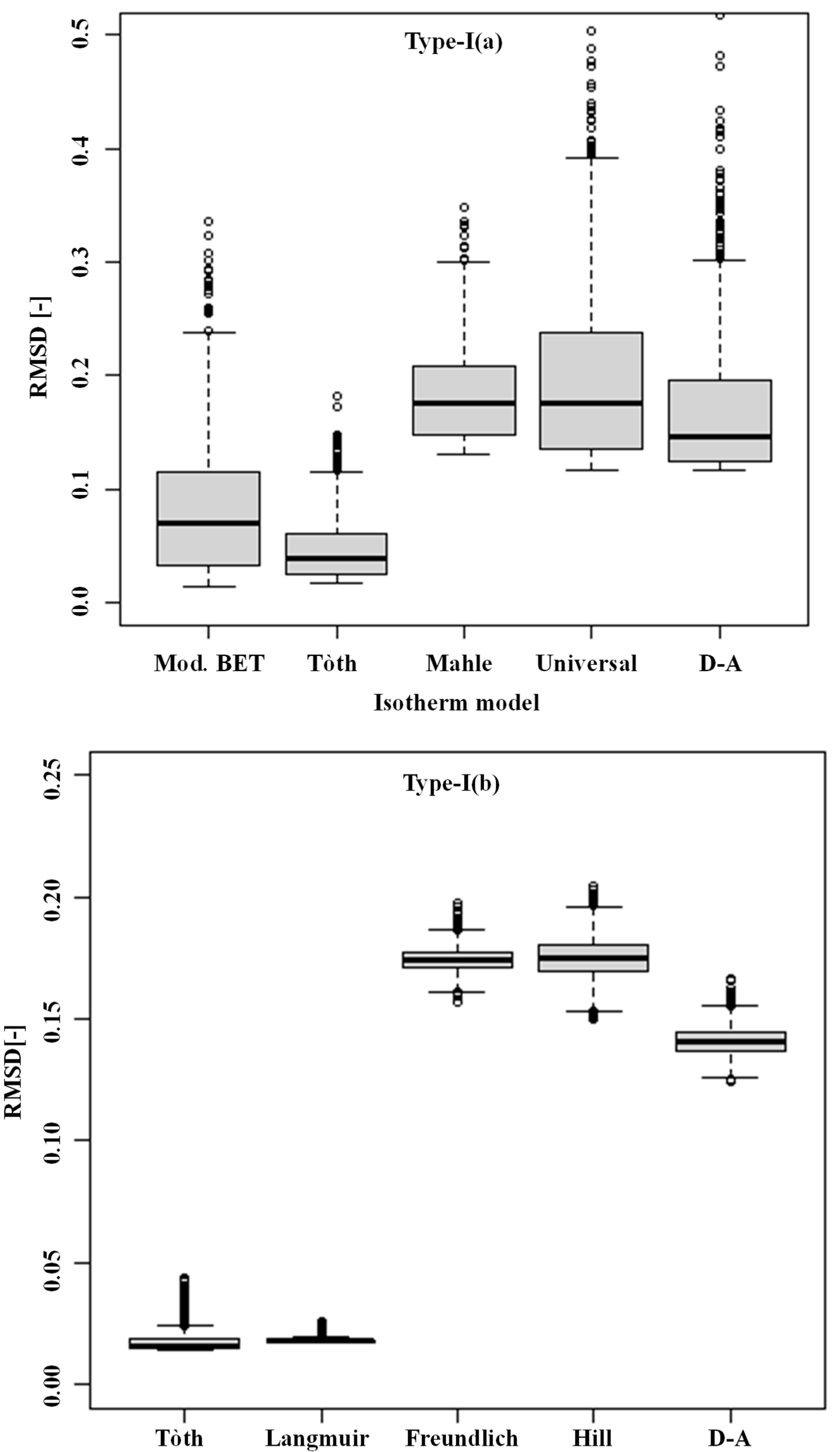
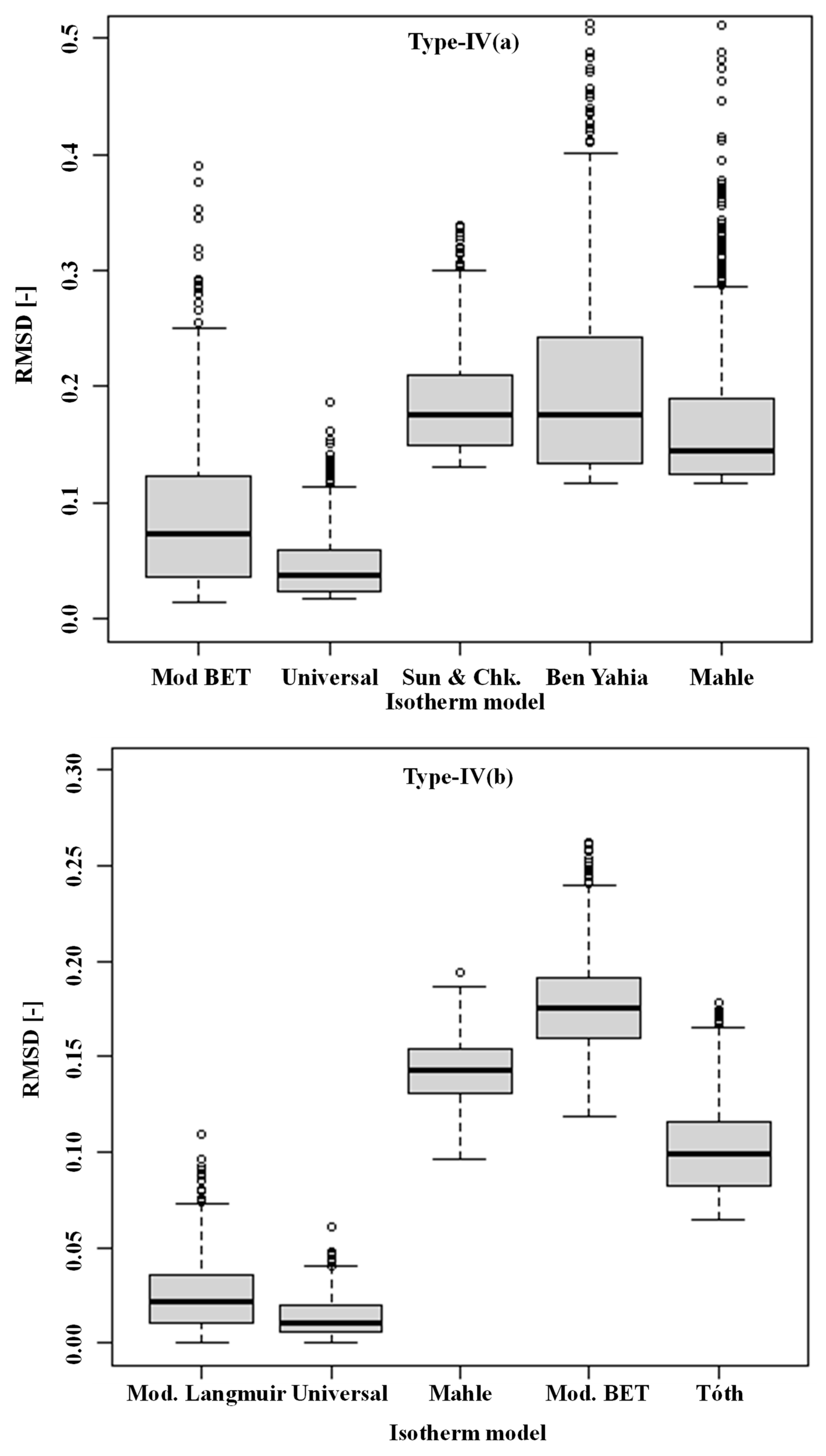
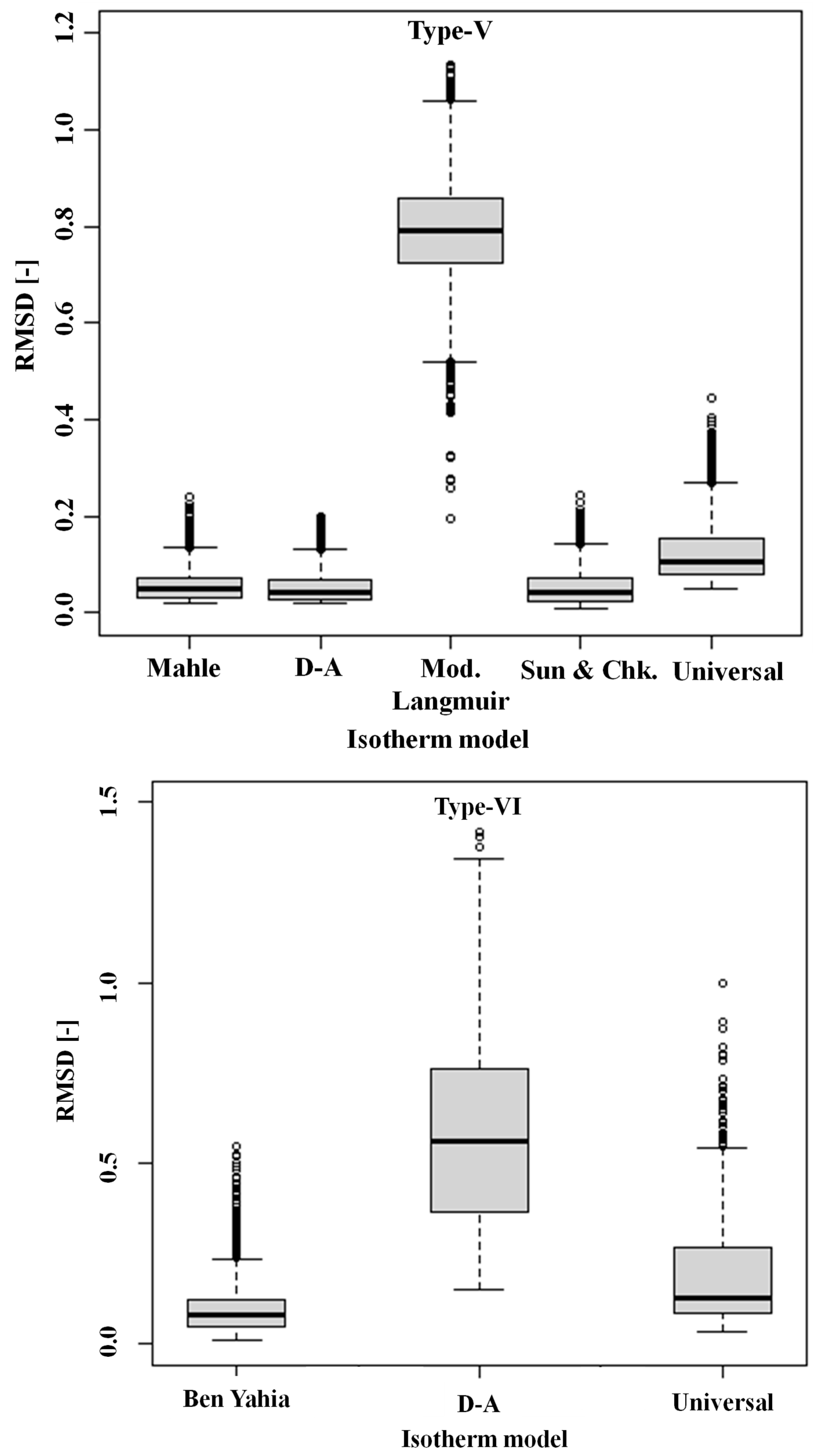
In the present study, n = 10,000 samples have been taken by varying parameters using the multivariate normal distribution, and for each case, errors have been calculated. The box-and-whisker plot was constructed using this error distribution and presented in Figure 3.

7.1. Box-and-Whisker Plot

Figure 3 shows the box-and-whisker plots using the observed RSMD of isotherm models for different types of isotherms. Each box plot demonstrates the distribution of RSMD estimates and their minimum, first quartile, median, third quartile, and maximum values. It is observed that in general, the distributions of RSMD estimations were positively skewed. However, the five-number summary of RSMD for the Tóth model was lower than other models for Type-I(a) and I(b) isotherms. Thus, the distribution of RSMD for the Tóth model was centered lower and less spread out compared to the candidate models. For type II isotherm the modified BET model is centered lower but spread out higher than other candidates. The results are similar in the case of Type-III isotherm where the GAB model also shows relatively lower values of median RSMD. The universal model is centered lower and less spread out than other models in the case of Type-IV(a) and IV(b) isotherms. In the case of Type-V isotherm, all models achieved a lower value of median and spread out less than the RSMD of the modified Langmuir model. The box plots for the Type-VI isotherm further show that the RSMD for Ben Yahia model was less spread out and centered lower than D-A and Universal models.
Based on Figure 3, it is therefore revealed that on average, the residuals of the Tóth model were relatively smaller and varied less compared to other models for Type-I(a). The finding was similar in the case of comparing the minimum, 1st quartile, 3rd quartile, maximum of Tóth model, and the other four candidates. Moreover, the Tóth model for Type-I(b), Mod BET model for Type-II, GAB model for Type-III, universal model for Type-IV(a) and Type-IV(b), Sun and Chakrabarty model for Type-V, and Ben Yahia model for Type-VI had the lower values of the five-number summary and dispersion compared to other models. Using the RSMD as a comparison criterion, these models were found better than other candidates in the respective isotherm cases. Table 3 presents the results of analysis of variance.

7.2. Non-Parametric Test: Kruskal–Wallis Rank-Sum Test

The non-parametric Kruskal–Wallis rank-sum test results containing degrees of freedom, chi-square statistic, and p-value are presented in Table 4.
In the ANOVA tests, the null hypothesis states that the average RMSD of five candidate isotherm models is equal for each type. Because the p-value is less than the significance level of 0.01, we can reject the null hypothesis for each type and conclude that some RMSD means of the models are different. So, in a particular type, all probable models are not equally likely, i.e., significantly differ. The null hypothesis of the non-parametric Kruskal–Wallis rank-sum test is similar to ANOVA, i.e., all candidate models for each type are equally fitted. The p-value is less than the significance level of 0.01, so the hypothesis is rejected at 1% level of significance, which implies all probable candidate models have different errors meaning that they are significantly different. To identify the best-fitted isotherm model, pairwise Tukey HSD test and Wilcoxon rank-sum test have been performed, and the results are shown in Table 5.
The null hypothesis of pairwise Tukey HSD test and non-parametric Wilcoxon rank-sum test state that each pair of models have equal RMSD means, indicating differences is zero. The p-values for these two tests are presented in Table 5 (Without parenthesis Tukey HSD and within parenthesis Wilcoxon rank-sum test). The p-value presented in Table 5 is very small, close to zero except for Sun and Chakrabarty vs. D-A of Type-V. So, all pairs of a specific type except Sun and Chakrabarty vs. D-A of Type-V are significantly different. So, based on the box-and-whisker plot and the overall and pairwise proportion test identified that Tóth for Type-I(a) and Type-I(b), modified BET for Type-II, GAB for Type-III, Universal model for Type-IV(a) and Type-IV(b), Sun and Chakraborty, and D-A models for Type-V, and Yahia et al. model for Type-VI are significantly optimum isotherm models.

7.3. Physical Description with Merit and Demerits of the IUPAC Isotherm Model

The Tóth model is determined to be the optimum for both Type-I(a) and Type-I(b) IUPAC isotherm. This model can be used to explain the monolayer adsorption process onto microporous adsorbents. Furthermore, the Tóth model well agrees in both Henry region and equilibrium at saturation. Whereas the Langmuir model only fits nicely in the low-pressure region, and the D-A model is well suited for the finite saturation region.
Type II isotherm is for monolayer and multilayer adsorption onto nonporous or macroporous adsorbents. Mod BET model is most suitable for all the pressure regions and this type of isotherm. Besides, D-A, Tóth, and universal models are close to the optimum model. The BET model fails to predict uptake around saturation pressure and can only be used to explain the multilayer adsorption process near saturation pressure.
The adsorbate–adsorbent interaction is rather weak in Type-III, and the adsorbed molecules cluster around the most favorable sites on the surface of a nonporous or macroporous material. The GAB model is most appropriate to explain this type of isotherm. GAB model is an upgrade of the modified BET model which considers all the assumptions of BET and modified BET model. Moreover, three other physical parameters are also included in this model that help to fit Type-III isotherms more accurately.
The interactions between the adsorbent and the adsorbate, as well as the interactions within the molecules in the condensed state, affect adsorption uptake onto the mesoporous adsorbent. The universal isotherm model, which includes two probability terms and an energy distribution parameter, has a high degree of agreement with Type-IV isotherms.
The Type-V isotherm is distinguished by its characteristic S-shaped form and the presence of a hysteresis loop. D-A, Tóth, and Langmuir models, in general, do not clarify the S-shaped isotherm within suitable error ranges. Sun and Chakrabarty model, on the other hand, considers (i) porous adsorbent materials structures, (ii) isosteric heat (Qst), and (iii) shape parameter (m) of the isotherms, all of which helps to explain the S-shape pattern.
The reversible stepwise Type-VI isotherm is characterized by layer-by-layer adsorption over a highly uniform non-porous surface. The energetic part of the Ben Yahia model is assumed to be dominant, and the adsorption process is divided into four energies. This model takes into account the number of molecules per receptor site, the density of receptor sites, and the molar adsorption energy of gases that correspond well with Type-VI isotherms.

7.4. Specific Cooling Effect (SCE)

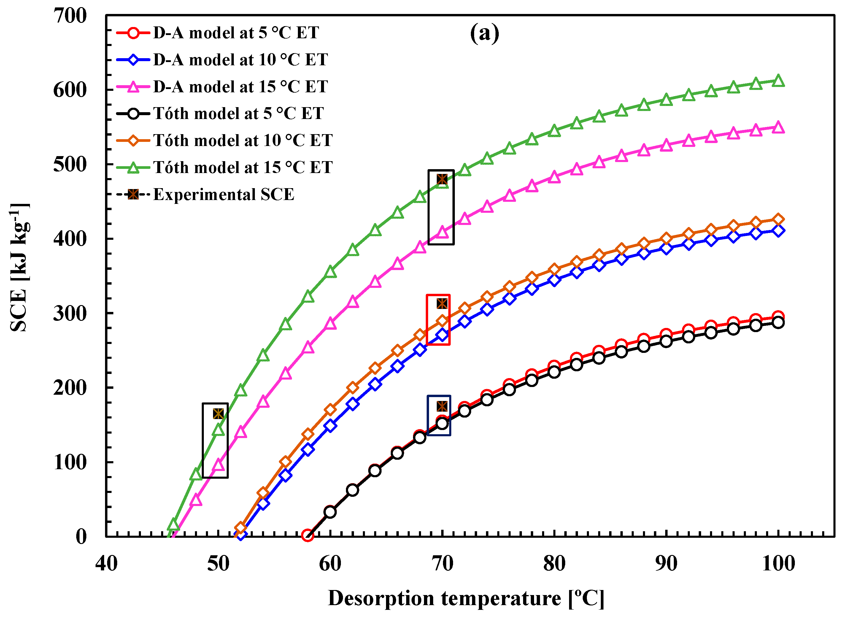
To validate this simulation study, two adsorption pairs, Maxsorb III/ethanol, and silica gel/water as Type-I(b) IUPAC isotherm, have been considered to calculate specific cooling effect (SCE) for cooling applications. The three most popular candidate models, namely, D-A, Tóth, and Langmuir model as Type-I(b) isotherms, have been considered to calculate the specific cooling effect (SCE). Figure 4 shows the SCE for Maxsorb III/ethanol and Figure 5 depicts SCE for silica gel/water pair for different evaporating temperatures considering desorption temperatures from 40 °C to 100 °C. Based on available experimental data, experimental SCE has been calculated and placed in Figure 4 and Figure 5. Figure 4a indicates that the SCE, using the Tóth model, is closer to the experimental SCE compared to the D-A model for Maxsorb III/ethanol pair. Similarly, in Figure 4b, the SCE for Maxsorb III/ethanol pair using the Tóth model is closer to the experimental SCE relative to the Langmuir model. For silica gel/water pair, it is found from Figure 5a,b that the SCE of the Tóth model is closer to the SCE measured from experimental data. So, it is concluded that the Tóth model is more efficient compared to other models as Type-I(b) IUPAC classified adsorption isotherm.

8. Conclusions

Relevant adsorption isotherm pairs for all of the IUPAC types are chosen for analysis in this study. Sensitivity analysis of the parameters has been performed and error is minimized to identify the optimum model. The experimental isotherm data, extracted from literature, are then fitted with different isotherm models through the GRG non-linear optimization method. This study provides simulation-based optimum model selection, where n = 10,000 samples were taken using multivariate normal distribution by varying parameters with a standard small range. Box-and-whisker plots are constructed by using 10,000 errors. Two overall mean test ANOVA and Kruskal–Wallis rank-sum test; two pairwise mean tests Tukey HSD and Wilcoxon rank-sum test confirms that Tòth for Type-I(a) and Type-I(b); modified BET for Type-II; GAB for Type-III; Universal for Type-IV(a) and Type-IV(b); Sun and Chakraborty and D-A for Type-V; and Ben Yahia for Type-VI are the significantly optimum models. The SCE measured by the Tòth model agrees well with the experimental SCE compared to the D-A and Langmuir models, indicating that the model suggested in this research is significantly optimum. Researchers can use the suggested optimum isotherms to execute a thorough investigation of adsorption cooling systems design.

Author Contributions

Conceptualization, M.M.R. and B.B.S.; Formal analysis, M.M.R., A.Z.S., M.A.I. and I.J.; Investigation, M.M.R., B.B.S. and A.P.; Methodology, M.M.R., I.J. and A.Z.S.; Software, M.M.R., A.Z.S. and I.J.; Supervision, B.B.S.; Validation, M.M.R., A.P. and M.A.I.; Writing—original draft, M.M.R. and A.Z.S.; Correction and revision of manuscript, M.M.R., A.P., M.A.I. and B.B.S. All authors have read and agreed to the published version of the manuscript.

Funding

This research did not receive any external funding.

Institutional Review Board Statement

Not applicable.

Informed Consent Statement

Not applicable.

Conflicts of Interest

The authors declare no conflict of interest.

References

  1. Saha, B.B.; Koyama, S.; Kashiwagi, T.; Akisawa, A.; Ng, K.C.; Chua, H.T. Waste heat driven dual-mode, multi-stage, multi-bed regenerative adsorption system. Int. J. Refrig. 2003, 26, 749–757. [Google Scholar] [CrossRef]
  2. Palomba, V.; Aprile, M.; Motta, M.; Vasta, S. Study of sorption systems for application on low-emission fishing vessels. Energy 2017, 134, 554–565. [Google Scholar] [CrossRef]
  3. Ng, K.C.; Thu, K.; Saha, B.B.; Chakraborty, A. Study on a waste heat-driven adsorption cooling cum desalination cycle. Int. J. Refrig. 2012, 35, 685–693. [Google Scholar] [CrossRef]
  4. Balaras, C.A.; Grossman, G.; Henning, H.-M.; Ferreira, C.A.I.; Podesser, E.; Wang, L.; Wiemken, E. Solar air conditioning in Europe—An overview. Renew. Sustain. Energy Rev. 2007, 11, 299–314. [Google Scholar] [CrossRef]
  5. Saha, B.B.; El-Sharkawy, I.I.; Shahzad, M.W.; Thu, K.; Ang, L.; Ng, K.C. Fundamental and application aspects of adsorption cooling and desalination. Appl. Therm. Eng. 2016, 97, 68–76. [Google Scholar] [CrossRef] [Green Version]
  6. Jaiswal, A.K.; Mitra, S.; Dutta, P.; Srinivasan, K.; Srinivasa Murthy, S. Influence of cycle time and collector area on solar driven adsorption chillers. Sol. Energy 2016, 136, 450–459. [Google Scholar] [CrossRef]
  7. Islam, M.A.; Saha, B.B. TEWI Assessment of Conventional and Solar Powered Cooling Systems. In Solar Energy; Tyagi, H., Ed.; Springer Nature: Singapore, 2020; pp. 147–177. ISBN 9789811506758. [Google Scholar]
  8. Muttakin, M.; Islam, M.A.; Malik, K.S.; Pahwa, D.; Saha, B.B. Study on optimized adsorption chiller employing various heat and mass recovery schemes. Int. J. Refrig. 2020, 126, 222–237. [Google Scholar] [CrossRef]
  9. Thommes, M.; Kaneko, K.; Neimark, A.V.; Olivier, J.P.; Rodriguez-Reinoso, F.; Rouquerol, J.; Sing, K.S.W. Physisorption of gases, with special reference to the evaluation of surface area and pore size distribution (IUPAC Technical Report). Pure Appl. Chem. 2015, 87, 1051–1069. [Google Scholar] [CrossRef] [Green Version]
  10. Rocky, K.A.; Pal, A.; Rupam, T.H.; Nasruddin; Saha, B.B. Zeolite-graphene composite adsorbents for next generation adsorption heat pumps. Microporous Mesoporous Mater. 2021, 313, 110839. [Google Scholar] [CrossRef]
  11. Jahan, I.; Rupam, T.H.; Palash, M.L.; Rocky, K.A.; Saha, B.B. Energy efficient green synthesized MOF-801 for adsorption cooling applications. J. Mol. Liq. 2021, 117760. [Google Scholar] [CrossRef]
  12. Rahman, M.M.; Muttakin, M.; Pal, A.; Shafiullah, A.Z.; Saha, B.B. A Statistical Approach to Determine Optimal Models for IUPAC-Classified Adsorption Isotherms. Energies 2019, 12, 4565. [Google Scholar] [CrossRef] [Green Version]
  13. Muttakin, M.; Mitra, S.; Thu, K.; Ito, K.; Saha, B.B. Theoretical framework to evaluate minimum desorption temperature for IUPAC classified adsorption isotherms. Int. J. Heat Mass Transf. 2018, 122, 795–805. [Google Scholar] [CrossRef]
  14. Pal, A.; Thu, K.; Mitra, S.; El-Sharkawy, I.I.; Saha, B.B.; Kil, H.S.; Yoon, S.H.; Miyawaki, J. Study on biomass derived activated carbons for adsorptive heat pump application. Int. J. Heat Mass Transf. 2017, 110, 7–19. [Google Scholar] [CrossRef]
  15. Nebaghe, K.C.; El Boundati, Y.; Ziat, K.; Naji, A.; Rghioui, L.; Saidi, M. Comparison of linear and non-linear method for determination of optimum equilibrium isotherm for adsorption of copper(II) onto treated Martil sand. Fluid Phase Equilib. 2016, 430, 188–194. [Google Scholar] [CrossRef]
  16. Ringot, D.; Lerzy, B.; Chaplain, K.; Bonhoure, J.P.; Auclair, E.; Larondelle, Y. In vitro biosorption of ochratoxin A on the yeast industry by-products: Comparison of isotherm models. Bioresour. Technol. 2007, 98, 1812–1821. [Google Scholar] [CrossRef]
  17. Do, D.D. Adsorption Analysis: Equilibria and Kinetics: (With CD Containing Computer Matlab Programs); Imperial College Press: London, UK, 1998; Volume 2, ISBN 978-1-78326-224-3. [Google Scholar]
  18. Sun, B.; Chakraborty, A. Thermodynamic frameworks of adsorption kinetics modeling: Dynamic water uptakes on silica gel for adsorption cooling applications. Energy 2015, 84, 296–302. [Google Scholar] [CrossRef]
  19. Kumar, K.V.; Porkodi, K. Relation between some two- and three-parameter isotherm models for the sorption of methylene blue onto lemon peel. J. Hazard. Mater. 2006, 138, 633–635. [Google Scholar] [CrossRef]
  20. Karmaker, S.C.; Eljamal, O.; Saha, B.B. Response surface methodology for strontium removal process optimization from contaminated water using zeolite nanocomposites. Environ. Sci. Pollut. Res. 2021. [Google Scholar] [CrossRef]
  21. Rahman, M.M.; Pal, A.; Uddin, K.; Thu, K.; Saha, B.B. Statistical Analysis of Optimized Isotherm Model for Maxsorb III/Ethanol and Silica Gel/Water Pairs. Evergreen 2018, 5, 1–12. [Google Scholar] [CrossRef]
  22. Askalany, A.A.; Saha, B.B.; Uddin, K.; Miyzaki, T.; Koyama, S.; Srinivasan, K.; Ismail, I.M. Adsorption isotherms and heat of adsorption of difluoromethane on activated carbons. J. Chem. Eng. Data 2013, 58, 2828–2834. [Google Scholar] [CrossRef]
  23. Amankwah, K.A.G.; Schwarz, J.A. A modified approach for estimating pseudo-vapor pressures in the application of the Dubinin-Astakhov equation. Carbon N. Y. 1995, 33, 1313–1319. [Google Scholar] [CrossRef]
  24. Pal, A.; Uddin, K.; Rocky, K.A.; Thu, K.; Saha, B.B. CO2 adsorption onto activated carbon–graphene composite for cooling applications. Int. J. Refrig. 2019, 106, 558–569. [Google Scholar] [CrossRef]
  25. Rocky, K.A.; Pal, A.; Moniruzzaman, M.; Saha, B.B. Adsorption characteristics and thermodynamic property fields of polymerized ionic liquid and polyvinyl alcohol based composite/CO2 pairs. J. Mol. Liq. 2019, 294, 111555. [Google Scholar] [CrossRef]
  26. Allen, S.J.; Gan, Q.; Matthews, R.; Johnson, P.A. Comparison of optimised isotherm models for basic dye adsorption by kudzu. Bioresour. Technol. 2003, 88, 143–152. [Google Scholar] [CrossRef]
  27. Berdenova, B.; Pal, A.; Saha, B.B.; Kaltayev, A. Non-isothermal pore change model predicting CO2 adsorption onto consolidated activated carbon. Int. J. Heat Mass Transf. 2021, 177, 121480. [Google Scholar] [CrossRef]
  28. Foo, K.Y.; Hameed, B.H. Insights into the modeling of adsorption isotherm systems. Chem. Eng. J. 2010, 156, 2–10. [Google Scholar] [CrossRef]
  29. Rahman, M.M.; Karmaker, S.C.; Pal, A.; Eljamal, O.; Saha, B.B. Statistical techniques for the optimization of cesium removal from aqueous solutions onto iron-based nanoparticle-zeolite composites. Environ. Sci. Pollut. Res. 2020, 28, 12918–12931. [Google Scholar] [CrossRef]
  30. Mahle, J.J. An adsorption equilibrium model for Type 5 isotherms. Carbon N. Y. 2002, 40, 2753–2759. [Google Scholar] [CrossRef]
  31. Peleg, M. Assessment of a semi-empirical four parameter general model for sigmoid moisture sorption isotherm. J. Food Process Eng. 1993, 16, 21–37. [Google Scholar] [CrossRef]
  32. Maroulis, Z.B.; Tsami, E.; Marinos-Kouris, D.; Saravacos, G.D. Application of the GAB model to the moisture sorption isotherms for dried fruits. J. Food Eng. 1988, 7, 63–78. [Google Scholar] [CrossRef]
  33. McMinn, W.A.M.; Magee, T.R.A. Thermodynamic properties of moisture sorption of potato. J. Food Eng. 2003, 60, 157–165. [Google Scholar] [CrossRef]
  34. Kayal, S.; Baichuan, S.; Saha, B.B. Adsorption characteristics of AQSOA zeolites and water for adsorption chillers. Int. J. Heat Mass Transf. 2016, 92, 1120–1127. [Google Scholar] [CrossRef]
  35. Zou, J.; Rezaee, R. A prediction model for methane adsorption capacity in shale gas reservoirs. Energies 2019, 12, 280. [Google Scholar] [CrossRef] [Green Version]
  36. Sun, B.; Chakraborty, A. Thermodynamic formalism of water uptakes on solid porous adsorbents for adsorption cooling applications. Appl. Phys. Lett. 2014, 104, 201901. [Google Scholar] [CrossRef]
  37. Yahia, M.B.; Khalfaoui, M.; Hachicha, M.A.; Lamine, A.B.; Torkia, Y.B.; Knani, S. Models for Type VI Adsorption Isotherms from a Statistical Mechanical Formulation. Adsorpt. Sci. Technol. 2013, 31, 341–357. [Google Scholar] [CrossRef]
  38. Aouaini, F.; Knani, S.; Ben Yahia, M.; Ben Lamine, A. Statistical physics studies of multilayer adsorption isotherm in food materials and pore size distribution. Phys. A Stat. Mech. Its Appl. 2015, 432, 373–390. [Google Scholar] [CrossRef]
  39. Ng, K.C.; Burhan, M.; Shahzad, M.W.; Ismail, A. Bin A Universal Isotherm Model to Capture Adsorption Uptake and Energy Distribution of Porous Heterogeneous Surface. Sci. Rep. 2017, 7, 1–11. [Google Scholar] [CrossRef] [Green Version]
  40. Saha, B.B.; Jribi, S.; Koyama, S.; El-Sharkawy, I.I. Carbon dioxide adsorption isotherms on activated carbons. J. Chem. Eng. Data 2011, 56, 1974–1981. [Google Scholar] [CrossRef]
  41. Vardeman, S.B.; Walpole, R.E.; Myers, R.H.; Miller, I.; Freund, J.E. Probability and Statistics for Engineers and Scientists. Probability and Statistics for Engineers; Pearson Education Inc.: Upper Saddle River, NJ, USA, 1986; Volume 81, ISBN 0132047675. [Google Scholar]
  42. Hogg, R.V.; Tanis, E.A.; Zimmerman, D.L. Probability and Statistical Interference; Pearson Education Inc.: Upper Saddle River, NJ, USA, 2003; ISBN 9780133936544. [Google Scholar]
  43. Saville, D.J. Multiple comparison procedures: The practical solution. Am. Stat. 1990, 44, 174–180. [Google Scholar] [CrossRef]
  44. Altman, D.G.; Bland, J.M. Practical statistics for medical research. BMJ 1995, 310, 170. [Google Scholar] [CrossRef] [Green Version]
  45. Siegel, S. Nonparametric Statistics. Am. Stat. 1957, 11, 13–19. [Google Scholar] [CrossRef]
  46. Liu, Y.; Chen, W. A SAS macro for testing differences among three or more independent groups using Kruskal-Wallis and Nemenyi tests. J. Huazhong Univ. Sci. Technol.-Med. Sci. 2012, 32, 130–134. [Google Scholar] [CrossRef] [PubMed]
  47. Bergmann, R.; Ludbrook, J. Different outcomes of the wilcoxon—mann—whitney test from different statistics packages. Am. Stat. 2000, 54, 72–77. [Google Scholar] [CrossRef]
  48. Uddin, K.; El-Sharkawy, I.I.; Miyazaki, T.; Baran Saha, B.; Koyama, S. Thermodynamic analysis of adsorption cooling cycle using ethanol-surface treated maxsorb III Pairs. Evergreen 2014, 1, 25–31. [Google Scholar] [CrossRef]
Figure 1. Types of adsorption isotherms [9,12]. (Reproduced with permission).
Energies 14 07478 g001
Figure 2. The box-and-whisker plot.
Energies 14 07478 g002
Figure 3. Box-and-whisker plots of the RMSD error (N = 10,000 simulated samples) were presented for all eight IUPAC classified isotherms.
Energies 14 07478 g003aEnergies 14 07478 g003bEnergies 14 07478 g003cEnergies 14 07478 g003d
Figure 4. Experimental SCE comparisons with, (a) Tóth vs. D-A, and (b) Tóth vs. Langmuir model of Maxsorb III/ethanol adsorption pair for different evaporating temperatures.
Energies 14 07478 g004aEnergies 14 07478 g004b
Figure 5. Experimental SCE comparisons with (a) Tóth vs. D-A models and (b) Tóth vs. Langmuir models of Silica gel/water adsorption pair for different evaporating temperatures.
Energies 14 07478 g005aEnergies 14 07478 g005b
Table 1. Non-linear adsorption isotherms models, parameters, and references.
IsothermNonlinear FormParametersReference
Freundlich W W 0 = ( P P s ) 1 n W0, n[14,15,16]
Langmuir W W 0 = b 0 e Q R T P 1 + b 0 e Q R T P W0, Q, b0[17,18,19,20]
D-A W W 0 = exp [ { R T E ln ( P s P ) } n ] W0, E, n[21,22]
Mod. (D-A) q a b s = W 0 V m exp [ { R T E ln ( P s P ) } n ] where, V m = V t exp [ α ( T T t ) ] and P s = ( T T c ) k P c W0, E, n, K[23,24]
Tόth W W 0 = b 0 e Q R T P 1 + b 0 e Q R T P W0, b0, Q, t[25,26,27]
Hill W W 0 = ( P P s ) n H K D + ( P P s ) n H W0, nH, KD[16,28,29]
Mahle W W s = 1 C [ tan 1 ( x A B ) tan 1 ( A B ) ] ; where, C = tan 1 ( 1 A B ) tan 1 ( A B ) and A = exp ( A 0 + A 1 T ) Ws, A0, A1, B[30]
BET V V m = C x ( 1 x ) ( 1 x + C x ) ; and x = P P 0 Vm, C[17,31]
Modified BET V V m = C K x ( 1 K x ) { ( 1 + ( C 1 ) K x ) } Vm, C, K[12,17]
GAB V V m = C K x ( 1 K x ) { 1 + ( C 1 ) K x } ; where, C = C 0 exp ( Δ H 1 R T ) ; K = K 0 exp ( Δ H 2 R T ) ; Δ H 1 = H m H n and Δ H 2 = H 1 H n Vm, C0, K0, ΔH1 and ΔH2[32,33]
Mod. Langmuir W W 0 = β ( P φ ) [ 1 + ( β m α ) ( P φ ) m ] 1 m ; Where, P φ = ( P P s ) exp { ϕ m R T { 1 ( P P s ) n } + z } W0, z, β, α, n1,
ϕm, m
[34,35]
Sun and Chakraborty W W 0 = K ( P P s ) m 1 + ( K 1 ) ( P P s ) m ; Where, K = α exp [ m ( Q s t h f g ) R T ] W0, Qst *, m, α[11,34,36]
Ben Yahia W = n 1 N M 1 ( P P 1 ) n 1 1 + ( P P 1 ) n 1 + n 2 N M 2 ( P P 2 ) n 2 1 + ( P P 2 ) n 2 + n 3 N M 3 ( P P 3 ) n 3 1 + ( P P 3 ) n 3 + n 4 N M 4 ( P P 4 ) n 4 1 + ( P P 4 ) n 4 ; and P i = P s exp ( E a i R T ) n1, n2, n3, n4, NM1, NM2, NM3, NM4, P1, P2, P3, P4[37,38]
Universal q q = i = 1 n α i [ ( p p s exp ( ε o i R T ) ) R T m i 1 + ( p p s exp ( ε o i R T ) ) R T m i ] i ; Where, α 1 + α 2 + α 3 + α 4 = 1 q*, αi, εoi, mi[13,39]
Table 2. Fitting parameters of the candidate models for Type-I(b) adsorption isotherm.
Type-I(a) (Carbon K4-700/N2 pair at 77 K)
ModelParameters
MahleW0 = 0.62, A0 = 0.045, A1 = −720, B = 0.01
UniversalW0 = 0.709, ε01 = 4120, ε02 = 0.0345, m1 = 320, m2 = 1000, α1 = 0.71, α2 = 0.29
D-AW0 = 0.607, E = 320, n = 3.31
TóthW0 = 0.61, b0 = 9.79 × 10⁻⁵, Q = 6013.84, t = 1.3
Mod BETVm = 0.594, C = 5334.78, k = 0.0446
Type-I(b) (Maxsorb III/ethanol)
FreundlichW0 = 1.482082, n = 2.214175
LangmuirW0 = 1.38, b0 = 3.10 × 10⁻⁹, Q = 48,600
D-AW0 = 1.17, E = 143.00, n = 1.9
TóthW0 = 1.2, b0 = 3.10 × 10⁻⁹, Q = 47,635, t = 1.69
Hill W0 = 1.266, nh = 1.321, KD = 0.080297
Type-II (Alumina/water)
Mod BETVm = 0.21, C = 25.5, k = 0.8186
UniversalW0 = 1.22, ε01 = 217.88, ε02 = 0.1762.69, m1 = 262.59, m2 = 3231.58, α1 = 0.42, α2 = 0.57
D-AW0 = 1.068, E = 73.72, n = 0.504
TóthW0 = 1.23, b0 = 2.32 × 10⁻³, Q = 16,932.30, t = 0.4165
LangmuirW0 = 0.891, b0 = 3.69 × 10⁻⁵, Q = 24,041.91
Type-III (Dried raisins/moisture)
GABVm = 10.517, C0 = 0.0011, K0 = 1.767, ΔH1 = 18.25, ΔH2 = −1.47
Mod BETVm = 10.421, C = 1.47, k = 0.980
UniversalW0 = 120, ε01 = 547.67, ε02 = 120.12, m1 = 199.95, m2 = 1846.68, α1 = 0.65, α2 = 0.35
Mod LangmuirW0 = 90.24, z = 0.1416, β = 0.0859, α = 0.958, n1 = 0.95, ϕm = 3.22, m = 0.7632
Sun and ChakrabartyW0 = 93.3581, Qst* = 3166.83, m = 2.449, α = 1.81 × 10⁻⁶
Type-IV(a) (PVDC/water)
UniversalW0 = 0.36, ε01 = 2096.47, ε02 = 5613.18, m1 = 478.42, m2 = 4025.91, α1 = 0.67, α2 = 0.33
Ben Yahian1 = 1.30, n2 = 0.13, n3 = 0.032, n4 = 1.3, NM1 = 0.123, NM2 = 0.150, NM3 = 0.495, NM4 = 0.399
Mod BETVm = 1.0533, C = 453.92, k = 0.00112
Sun and ChakrabartyW0 = 0.341, Qst* = 3497.21, m = 2.099, α = 9.00 × 10⁻⁷
MahleW0 = 0.35, A0 = 0.89, A1 = −575, B = 0.2
Type-IV(b) (IRMOF-74-V-hex/nitrogen)
UniversalW0 = 2.85, ε01 = 852.32, ε02 = 2364.60, m1 = 138.23, m2 = 608.42, α1 = 0.54, α2 = 0.46
Mod BETVm = 0.21, C = 28, k = 0.8186
MahleW0 = 0.21, A0 = 0.6, A1 = −650, B = 0.075
Mod LangmuirW0 = 80, z = 0.119, β = 0.03622, α = 0.9941, n1 = 0.98, ϕm = 3.22, m = 0.478
TóthW0 = 2.9, b0 = 0.0001041, Q = 4302.19, t = 1.3183
Type-V (FAM-Z01/water)
Sun and ChakrabartyW0 = 0.2042, Qst* = 3027.841, m = 4.893, α = 9 × 10⁻⁷
Mod LangmuirW0 = 0.210, z = 2.955, β = 0.60086, α = 0, n1 = −1.5, ϕm = 510.79, m = 1.82
MahleW0 = 0.21, A0 = 0.60, A1 = −650, B = 0.075
DAW0 = 0.212, E = 3985.785, n = 3.7075
UniversalW0 = 0.25, ε01 = 3841.16, ε02 = 0.01, m1 = 530.08, m2 = 2583.121, α1 = 0.67, α2 = 0.33
Type-VI (MgO/methane)
UniversalW0 = 12, ε01 = 3450, ε02 = 1015.22, ε03 = 235, ε04 = 45, m1 = 342, m2 = 24.96, m3 = 135.21, m4 = 93.44, α1 = 0.062, α2 = 0.05, α3 = 0.55, α4 = 0.40
Ben Yahia n1 = 2.95, n2 = 19.52, n3 = 77.27, n4 = 23.26, NM1 = 0.252, NM2 = 0.036, NM3 = 0.007, NM4 = 0.071, P1 = 0.70, P2 = 20.82, P3 = 36.06, P4 = 47.10
Mod. LangmuirW0 = 4, z = 4.38, β = 0.044, α = 0.033, n1 = −1.5, ϕm = 44.77, m = 0.683
MahleW0 = 4.457, A0 = 2.013 × 10⁻⁵, A1 = 62.92, B = 0.0927
D-AW0 = 4.012, E = 1219.71, n = 0.9
Table 3. Parametric Test: Analysis of Variance (ANOVA).
DFSSMean SSF-Valuep-Value
Type-I(a)4261.7265.432,532,683<2 × 10⁻¹⁶ ***
Type-I(b)425.236.3088452<2 × 10⁻¹⁶ ***
aType-II382.6927.56306,633<2 × 10⁻¹⁶ ***
Type-III424.356.08752534<2 × 10⁻¹⁶ ***
Type-IV(a)44896122452,346<2 × 10⁻¹⁶ ***
Type-IV(b)4112.9528.2349,863<2 × 10⁻¹⁶ ***
Type-V441841046318,711<2 × 10⁻¹⁶ ***
Type-VI43524.18881.04214,241<2 × 10⁻¹⁶ ***
*** denote 1% level of significance.
Table 4. Chi-square (χ2) and p-value of Kruskal–Wallis rank-sum test results.
TypedfChi-Square (χ2)p-Value
Type-I(a)425,3562.16 × 10−13
Type-I(b)443,6362.21 × 10−14
Type-II328,2962.22 × 10−16
Type-III454,2631.48 × 10−11
Type-IV(a)435,4212.25 × 10−13
Type-IV(b)429,6533.25 × 10−15
Type-V424,8062.20 × 10−16
Type-VI435,4122.22 × 10−16
Table 5. p-value of pairwise test results. Without parenthesis Tukey HSD and within parenthesis Wilcoxon rank-sum test.
Type-I(a)
ModelTóthD-AMod BETUniversal
D-A1.7 × 10−7 (2.61 × 10⁻⁸)---
Mod BET1.6 × 10−9 (1.96 × 10⁻¹⁶)1.8 × 10⁻¹⁵ (2.21 × 10⁻¹⁶)--
Universal1.8 × 10−7 (1.35 × 10⁻¹⁶)0.00360 (2.31 × 10⁻¹⁶)2.2 × 10⁻¹¹ (2.36 × 10⁻¹⁶)
Mahle3.1 × 10−4 (2.34 × 10⁻¹⁶)2.1 × 10⁻¹² (1.74 × 10⁻¹⁶)1.2 × 10⁻⁵ (2.23 × 10⁻¹⁶)2.9 × 10⁻⁷ (5.3 × 10⁻¹⁶)
Type-I(b)
TóthLangmuirFreundlichHill
Langmuir1.3 × 10−11 (2 × 10⁻¹⁶)---
Freundlich2.3 × 10−13 (2 × 10⁻¹⁶)2.5 × 10⁻⁸ (2 × 10⁻¹⁶)--
Hill0.00021 (2 × 10⁻¹⁶)4.2 × 10⁻⁵ (2 × 10⁻¹⁶)1.8 × 10⁻¹⁶ (2 × 10⁻¹⁶)
D-A0.00032 (2 × 10⁻¹⁶)2.3 × 10⁻⁶ (2 × 10⁻¹⁶)3.2 × 10⁻¹⁶ (2 × 10⁻¹⁶)2.6 × 10⁻⁸ (2 × 10⁻¹⁶)
Type-II
Mod BETUniversalD-A
Universal2.1 × 10−15 (2 × 10⁻¹⁶)--
D-A0.00898 (2 × 10⁻¹⁶)1.6 × 10⁻¹⁴ (2 × 10⁻¹⁶)-
Tóth3.5 × 10−12 (2 × 10⁻¹⁶)3.5 × 10⁻¹⁵ (2 × 10⁻¹⁶)2.6 × 10⁻¹¹ (2 × 10⁻¹⁶)
Type-III
GABMod BETUniversalD-A
Mod BET1.9 × 10−16 (2.10 × 10⁻¹⁶)---
Universal2.3 × 10−14 (1.96 × 10⁻¹⁶)6.5 × 10⁻¹⁴ (2.21 × 10⁻¹⁶)--
D-A5.9 × 10−14 (1.35 × 10⁻¹⁶)2.3 × 10⁻¹³ (2.31 × 10⁻¹⁶)3.1 × 10⁻¹² (2.36 × 10⁻¹⁶)
Sun and Chk2.6 × 10−15 (2.34 × 10⁻¹⁶)3.5 × 10⁻¹⁴ (1.74 × 10⁻¹⁶)2.8 × 10⁻¹⁵ (2.23 × 10⁻¹⁶)2.4 × 10⁻¹⁴ (5.3 × 10⁻¹⁶)
Type-IV(a)
Mod BETUniversalSun and ChkBen Yahia
Universal2.3 × 10−8 (2.10 × 10⁻¹⁶)---
Sun and Chk1.8 × 10−9 (1.96 × 10⁻¹⁶)3.4 × 10⁻¹⁰ (2.21 × 10⁻¹⁶)--
Ben Yahia3.6 × 10−11 (1.35 × 10⁻¹⁶)2.4 × 10⁻¹³ (2.31 × 10⁻¹⁶)2.7 × 10⁻¹⁵ (2.36 × 10⁻¹⁶)
Mahle2.8 × 10−8 (2.34 × 10⁻¹⁶)3.1 × 10⁻¹⁰ (1.74 × 10⁻¹⁶)2.5 × 10⁻¹⁰ (2.23 × 10⁻¹⁶)3.2 × 10⁻¹⁶ (5.3 × 10⁻¹⁶)
Type-IV(b)
Mod LangmuirUniversalMahleMod BET
Universal2.4 × 10−15 (2.10 × 10⁻¹⁶)---
Mahle2.3 × 10−14 (1.96 × 10⁻¹⁶)1.4 × 10⁻¹⁵ (2.21 × 10⁻¹⁶)--
Mod BET2.1 × 10−12 (1.35 × 10⁻¹⁶)1.9 × 10⁻¹³ (2.31 × 10⁻¹⁶)2.2 × 10⁻¹² (2.36 × 10⁻¹⁶)
Tóth2.5 × 10−14 (2.34 × 10⁻¹⁶)3.4 × 10⁻¹¹ (1.74 × 10⁻¹⁶)3.4 × 10⁻¹⁶ (2.23 × 10⁻¹⁶)2.4 × 10⁻¹⁶ (5.3 × 10⁻¹⁶)
Type-V
MahleD-AUniversalSun and Chk
D-A2.1 × 10−10 (7.98 × 10⁻⁴)---
Universal3.1 × 10−12 (1.96 × 10⁻¹⁶)1.8 × 10⁻⁹ (2.21 × 10⁻¹⁶)--
Sun and Chk2.7 × 10−5 (1.13 × 10⁻⁴)0.7158 (0.35142)2.3 × 10⁻⁸ (2.36 × 10⁻¹⁶)
Mod Langmuir2.7 × 10−14 (2.34 × 10⁻¹⁶)1.6 × 10⁻¹² (1.74 × 10⁻¹⁶)3.4 × 10⁻¹⁵ (2.23 × 10⁻¹⁶)2.9 × 10⁻¹³ (5.3 × 10⁻¹⁶)
Type-VI
Ben YahiaUniversalD-AMod. Langmuir
Universal2.2 × 10−2 (2.10 × 10⁻³)---
D-A3.1 × 10−12 (2.56 × 10⁻¹²)1.3 × 10⁻¹² (3.21 × 10⁻¹²)--
Mod. Langmuir3.6 × 10−10 (2.51 × 10⁻¹³)3.9 × 10⁻¹⁰ (5.23 × 10⁻⁸)3.5 × 10⁻¹⁰ (7.65 × 10⁻⁸)
Mahle2.8 × 10−9 (3.51 × 10⁻¹¹)4.3 × 10⁻⁷ (1.74 × 10⁻¹²)3.2 × 10⁻¹² (4.23 × 10⁻¹¹)3.6 × 10⁻¹⁴ (3.3 × 10⁻¹³)
Publisher’s Note: MDPI stays neutral with regard to jurisdictional claims in published maps and institutional affiliations.