Resilience Assessment: A Performance-Based Importance Measure

Abstract

The resilience of a system can be considered as a function of its reliability and recoverability. Hence, for effective resilience management, the reliability and recoverability of all components which build up the system need to be identified. After that, their importance should be identified using an appropriate model for future resource allocation. The critical infrastructures are under dynamic stress due to operational conditions. Such stress can significantly affect the recoverability and reliability of a system’s components, the system configuration, and consequently, the importance of components. Hence, their effect on the developed importance measure needs to be identified and then quantified appropriately. The dynamic operational condition can be modeled using the risk factors. However, in most of the available importance measures, the effect of risk factors has not been addressed properly. In this paper, a reliability importance measure has been used to determine the critical components considering the effect of risk factors. The application of the model has been shown through a case study.

1. Introduction

Critical infrastructures are complex systems whose high performance requires proper interaction between hardware, software, and wetware (humans being involved in the design and operation of these systems). External and internal working of infrastructures is dynamic, which constantly can change the performance characteristics of these systems. For example, dynamic operational conditions can affect equipment reliability and recoverability, two characteristics of infrastructure resilience (see Figure 1). Changing the reliability can cause an unexpected breakdown. For example, ambient temperature effects on the reliability and recoverability of power distribution have a dynamic nature, and a sudden low temperature will cause an unexpected power outage. Such unexpected stoppages need to be considered in any contingency plan. Moreover, it is important to clearly understand each component’s importance in building critical infrastructures and their sensitivity to any change in operational conditions.

Recently, different resilience metrics have been developed to assess the resilience of systems in different sectors. Figure 1 shows some of the concepts of resilience and some key concepts, which have been used to represent the system statement pre-disruption, during disruption, and post-disruption. Resilience is a technical system that can be defined as the ability to withstand a major disruption within acceptable degradation parameters and recover within an acceptable time and composite costs and risks [1,2].

In other words, resilience could be interpreted as the probability that system conditions might exceed an irrevocable tipping point. But the probability in this subject covers the different areas that different approaches and indices can evaluate. The reliability (uptime) and recoverability (downtime) performance have been used as the most dominant probabilistic performance measurement tools. As Figure 1 shows, the reliability of the system resilience in the original stable state before a disruption occurs starts from the time to (normal or baseline state). Reliability is defined as the probability that a system can perform a required function under given conditions at a given instant of time or over a given time interval, assuming the required external resources are provided [3,4,5,6,7,8,9,10]. At the time of $t_1$ the system will be hit by a disruptive event (overstress such as an earthquake). Based on the inherent reliability and effectiveness of the operation and maintenance program, the performance of the system will degrade until $t_2$. Some authors highlighted that as a vulnerability state, where higher vulnerability means more severe failure. At the time $t_2$ the contingency plan (recovery actions) is in place, and the system’s recoverability will decide when the system will get back to the normal performance level [11].

One important step in improving infrastructure resilience is identifying the critical components that contribute to its resilience. The component importance can be identified from a reliability and recoverability point of view. Different reliability importance measures have been developed, which may be used in the resilience assessment as well. The importance measure denotes how each component will affect the infrastructure performance. In general, the resilience importance results from its component’s resilience through the cohesive configuration components interacting. Therefore, a two-dimensional index that measured both resilience and each components’ behavior in interaction with other components and the system needs to be developed to analyze the system. Such indexes are known as importance measures obtained from the reliability of the recoverability point of view. Different importance measures have been developed in the reliability of the engineering discipline. For example, Birnbaum (1968) proposed a quantitative definition of structural importance for systems with coherent structures, assuming that only the complex system’s structure is known. Chang and Hwang used structural Birnbaum importance in the component assignment problem to obtain the best system reliability [12,13,14]. Amrutkar and Kamalja overviewed structural importance measures, reliability importance measures, and lifetime importance measures of importance measures for coherent systems from 1960 to 2017 [15]. A resilience-focused performance measure was offered through generated interdependent power-water networks by Almoghathawi and Barker [16]. Chacko introduced joint reliability importance measure for two or more multistate components, joint performance achievement worth, joint performance reduction worth, and the joint performance Fussell–Vesely measure, using expected performance, reliability, availability, and risk as output performance measures of the multistate system [17]. Xu et al. used the values of component importance to investigate a time-dependent risk quantification model, as well as the common cause failure treatment model in operation and maintenance management. The results showed that the absolute values and ranking order of time-dependent importance reflected the effect of the cumulative state duration of component on risk and comprehensively accounted for all possible situations of component unavailability [18]. Kamra and Pahuja analyzed the substation communication network architectures using various reliability importance measures. The practice of these component importance measures worked towards identifying the components that can be allocated for the improvement of system reliability [19]. Niu et al. extended the component importance to generating capacity adequacy assessment. The measurement index is the centrepiece in reliability importance based on traditional importance measures. It is demonstrated that a central component, the one with higher structure importance, can actually have less risk reduction worth than a branch, the one with lower structure importance [20]. Furthermore, some authors proposed the availability importance measure (AIM), which determines the importance of items regarding the availability of the mechanical system and smart grid (regarded as the next-generation electrical power grid).

A review of available studies revealed that in most available studies, the reliability of components depends on a single independent variable, time of operation, or time between failures (TBF). Moreover, these studies mostly assume that the data are homogenous, where the data are collected under identical operational conditions. Here, the equipment is experiencing the same operational conditions with the same environmental, operational and organizational stress. In reality, it is not a valid assumption. Studies show that most of the resilience data have a degree of heterogeneity that needs to be identified and quantified appropriately. In other words, operational conditions can significantly influence the infrastructures’ reliability and recoverability characteristics in most real cases.

In general, risk factors could be categorized into two groups, observable and unobservable risk factors leading to observable and unobservable heterogeneity. Unobservable risk factors are such factors that they are unknown. Recent studies show that the unobservable risk factors can significantly change the components’ reliability and recoverability and, consequently, the resilience characterization of infrastructures. Hence, the effect of both observable and unobservable risk factors should be considered while the component importance measure is analysing [21,22,23,24,25,26,27]. However, in most of the available importance measures, the effect of risk factors has not been addressed properly. Recently, different approaches have been used to analyze the effect of risk factors on system resilience, such as regression methods, neural networks, classical statistics, etc. [28,29,30]. For example, Cox regression and accelerator failure time (AFT) models are the two most applied regression models for modelling the effect of risk factors on the resilience of infrastructures [11,21,22,31]. In these models, reliability or recoverability can be explored as baseline hazard/repair rate and covariate function, reflecting the effect of risk factors on the baseline hazard rate. Baseline hazard represents the hazard when all of the risk factors (or predictors or independent variables) effects (coefficient values) are equal to zero [25].

Hence, the main motivation of this paper is to develop risk factors-reliability importance measures to isolate the effect of observable and unobservable risk factors. The paper is divided into three parts. Part 2 briefly presents the theoretical background for “risk factor-based reliability importance measure (RF-RIM)”. Moreover, the methodology for the implementation of the model is discussed. Part 3 presents a case study featuring the reliability importance analysis part of the fleet loading system in Iran’s ore mine. Finally, part 4 provides the conclusion of the paper.

2. Methodology and Framework: Risk Factor-Based Reliability Importance Measure (RF-RIM)

Mathematically, the resilience measure can be defined as the sum of reliability and recoverability (restoration) as follows [32]:

$$Re = R\left(reliability\right) + \rho \left(restoration\right) = R + \rho \left(R,{\mathsf{\Lambda }}_p,{\mathsf{\Lambda }}_D,K\right)$$

(1)

where k, ${\mathsf{\Lambda }}_p and{ \mathsf{\Lambda }}_D$ are the conditional probabilities of the mitigation/recovery action success, correct prognosis, and diagnosis. Equation (1) turns technical infrastructure resilience into a quantifiable property; provides essential information for managing them efficiently. Reliability is defined as the probability that a system can perform a required function under given conditions at a given instant of time, assuming the required external resources are provided [12]. The reliability can be model using a statistical approach such as classical distribution. The restoration is considered as a joint probability of having an event, correct prognosis, diagnosis, and mitigation/recovery as follows [33]:

$$Re = R + \left(1 - R\right)P_{Diagonosis}{P}_{Prognosis}{P}_{Recovery}$$

(2)

where $P_{Diagonosis}$ is the probability of correct diagnosis, $P_{Prognosis}$ is the probability of correct prognosis, and $P_{Recovery}$ is the probability of correct recovery [32].

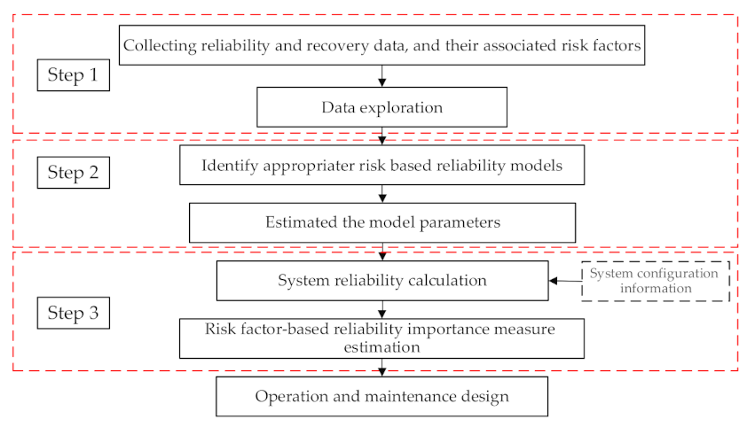
As mentioned, the importance measure shows how to affect each component on the system resilience. For example, in a series system, components to have the least reliability, the most effective have on the system resilience. However, in a parallel system, components that have the most reliability are the most effective on the system resilience. Figure 2 shows a systematic guideline for RF-RIM.

As this figure shows, the initial step involves collecting failure and repair data and their associated risk factors. The most important challenge in the first step is the quality and accuracy of the collected data set, which significantly affects the analysis results [28]. In the second step, based on the nature of the collected data and risk factors, some statistical models are nominating to model the reliability of components. For example, in the presence of observable and unobservable risk factors, the frailty model can be used. Originally, this was developed by Asha et al. [34] into load share systems and described the effect of observable and unobservable covariates on the reliability analysis. In later years, authors such as Xu and Li, Misra et al., and Giorgio et al. discussed the properties of the frailty model [35,36,37]. Moreover, recently this model was used in spar part estimation, remaining useful life (RUL), recoverability, failure data analysis, and resilience analysis [21,22,23,24,38,39]. According to this model, the reliability of each component $\left(R\left(t;z;z\left(t\right)|\alpha \right)\right)$ can be modelled as follows [21,22,23,24]:

$$R_i\left(t;z;z\left(t\right)|\alpha \right) = {\left\{R_i\left(t;z;z\left(t\right)\right)\right\}}^{\alpha }$$

(3)

where $\alpha$ is the frailty and has a probability density function g(α) with the mean to one and variance θ, where $R_i\left(t;z;z\left(t\right)\right)$ is the item’s reliability function and considering the existence of p₁ time-independent observable risk factors and p₂ time-dependent observable risk factors. It can be estimated by [21,22,23,24]:

$$R_i\left(t;z;z\left(t\right)\right) = {\left[exp\left(-\underset{0}{\overset{t}{{\displaystyle \int }}}{\lambda }_0\left(x\right)exp\left[{\displaystyle \sum }_{j = 1}^{p_2}{\delta }_{sj}{z}_{sj}\left(t\right)\right]dx\right)\right]}^{\exp \left[{\displaystyle \sum }_{i = 1}^{p_1}{\eta }_{si}{z}_{si}\right]}$$

(4)

where ${\lambda }_0$ is baseline hazard rate. Also, $\delta$ and $\eta$ are regression coefficients of the corresponding time-independent and observable risk factors. Moreover, the unconditional reliability function of component i’th $\left(R_{\theta i}\left(t;z;z\left(t\right)\right)\right)$ can be estimated as [21,22,23,24]:

$$R_{\theta i}\left(t;z;z\left(t\right)\right) = {\displaystyle {\int }_0^{\infty }}{\left\{R_i\left(t;z;z\left(t\right)\right)\right\}}^{\alpha }g\left(\alpha \right)d\alpha = {\left[1 - {\theta }_{i}ln\left\{R_i\left(t;z;z\left(t\right)\right)\right\}\right]}^{\raisebox{1ex}{$-1$}\!\left/ \!\raisebox{-1ex}{${\theta }_i$}\right.}$$

(5)

where $R_{\theta i}\left(t;z;z\left(t\right)\right)$ is the item’s reliability function and considering the existence of observable and unobservable risk factors. If there is no effect from unobservable risk factors, then $\alpha$ = 1, and Equation (6) will reduce to the Cox regression model as follows [22,31,39]:

$$R_{\theta i}\left(t;z;z\left(t\right)\right) = {\displaystyle {\int }_0^{\infty }}{\left\{R_i\left(t;z;z\left(t\right)\right)\right\}}^{\alpha }g\left(\alpha \right)d\alpha = {\left[1 - {\theta }_{i}ln\left\{R_i\left(t;z;z\left(t\right)\right)\right\}\right]}^{\raisebox{1ex}{$-1$}\!\left/ \!\raisebox{-1ex}{${\theta }_i$}\right.}$$

(6)

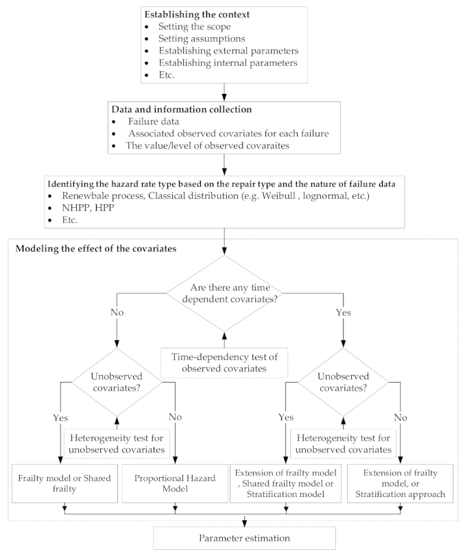
For a guideline in risk factor-based reliability model selection, see Figure 3.

In step 3, the system reliability should be estimated. In the presence of observable and unobservable risk factors, for a series-parallel system with n series and m parallel subsystems, system reliability can be calculated with Equation (7) [21,22,40]:

$$R_s\left(t;z;z\left(t\right)|\alpha \right) = {\displaystyle \prod }_{i = 1}^n\left[1 - \left[{\displaystyle \prod }_{j = 1}^{m}1 - R_{\theta ij}\left(t;z;z\left(t\right)|\alpha \right)\right]\right]$$

(7)

where, $R_s\left(t;z;z\left(t\right)|\alpha \right)$ is system reliability at time t, z is a row vector consisting of the observable time-independent risk factors, z(t) is a row vector consisting of the observable time-dependent risk factors and ${\alpha }_j$ are a time-independent frailty function for item j and represents the cumulative effect of one or more unobservable risk factors [21,22,41], $R_{ij}\left(t\right)$ is component reliability at time t. having the reliability model of the system the reliability importance measure of components that are working in a series-parallel system can be estimated by:

$${\mathrm{I}}_{\mathrm{R}}^i\left(t;z;z\left(t\right)|\alpha \right) = \frac{\partial {\mathrm{R}}_{\mathrm{s}}\left(t;z;z\left(t\right)|\alpha \right)}{\partial {\mathrm{R}}_i\left(t;z;z\left(t\right)|\alpha \right)}$$

(8)

where ${\mathrm{I}}_{\mathrm{R}}^i$ and ${\mathrm{R}}_{\mathrm{i}}$ are RF-RIM and reliability of component considering by observable and unobservable risk factors.

3. Case Study

Mining is an important industry that provides raw materials, which are an essential input for other industries. Gol-Gohar iron ore mine is located in southern Iran, in the southwest of Kerman province. Gol-Gohar iron ore mine contains six sections. Each of them works independently. Mining in surface mines starts by drilling the rock, blasting, loading, and then transforming the rock to the production facility or a depot. Nowadays, the mining industry uses huge equipment to increase performance. Extraction equipment is very expensive; any unplanned stopped may cause tremendous costs.

Moreover, long stoppages may affect the ore processing facilities, which are downstream of the production chain. Recently, the resilience concept has instructed the mining industries to avoid any disturbance in the chain of production. A previous study showed that Gol-Gohar operational conditions could significantly affect the resilience characteristics of mining equipment. To manage resilience effectively, we need to measure different quality, net considering, and operational conditions. Hence, in this study, we used the RF-RIM developed in Section 2 on the transience of the loading fleet, including four Caterpillar (Caterpillar Inc. Construction machinery and equipment company, Deerfield, IL, USA) excavators model 390DL in section No. 1.

3.1. Data Collection and Classification

According to the guideline developed in Figure 2, the first step is to collect the data. The data required for reliability analysis can be divided into two categories: failure data and risk factors. In this case, failure data (time to failures) and their possible associated risk factors were collected from January 2016 to December 2018. These data are collected from various sources, including daily operation reports, mounted sensors on the machine, meteorology reports, geological specifications, and interviews with experts, meetings, archival documents (previous reports, machines catalogs). Collected risk factors include qualitative (categorical) and quantitative (continuous) risk factors. Continuous risk factors include: temperature ($Z_5$), precipitation ($Z_4$), and humidity ($Z_6$). The categorical risk factors include working shift ($Z_1$), rock kind ($Z_2$) and operation team ($Z_3$).

Table 1. The classification and quantification of qualitative risk factors.

Risk Factors (z)	Classification	Quantification
Shift ($Z_1$)	Morning	1
	Afternoon	2
	Night	3
Rock kind ($Z_2$)	Waste	1
	Ore	2
Operation team ($Z_3$)	A	1
	B	2
	C	3
	D	4
Precipitation ($Z_4$)	Continues
$\mathrm{Temperature} (Z_5$)	Continues
$\mathrm{Humidity} (Z_6$)	Continues

shows the formulation of the categorical risk factors. For example, this table shows shift has three categories: morning, afternoon, and night, and 1, 2, 3 represent them, respectively.

3.2. Risk Factor Test

Two tests have been carried out on 10 collected risk factors, correlation test, and PH assumption in this part. Correlation tests are performing to find if the identified risk factors are independent of each other. If there are some independent risk factors, they should be replaced by new risk factors built up based on independent risk factors. Furthermore, time dependency is checking to find the effect of some risk factor changing which time. Such tests are named the PH-assumption test.

Here the Pearson test is used for checking the correlation between risk factors. The risk factors correlation test for excavators showed there is no significant correlation between an identified risk factor. As an example,

Table 2. The checking correlation between risk factors for excavator A.

Correlation		${\mathrm{Z}}_1$	${\mathrm{Z}}_5$	${\mathrm{Z}}_4$	${\mathrm{Z}}_2$	${\mathrm{Z}}_3$
${\mathrm{Z}}_1$	Pearson value.	1	−0.04	.	0.11	−0.01
	p-value		0.45	.	0.04	0.83
${\mathrm{Z}}_5$	Pearson value	−0.04	1	.	−0.11	0.02
	p-value	0.45		.	0.04	0.68
${\mathrm{Z}}_4$	Pearson value	.	.	.	.	.
	p-value	.	.	.	.	.
${\mathrm{Z}}_2$	Pearson value	0.11	−0.11	.	1	−0.08
	p-value	0.04	0.04	.		0.15
${\mathrm{Z}}_3$	Pearson value	−0.01	0.023	.	−0.08	1
	p-value	0.83	0.68	.	0.15

shows such results for excavator A. As can be seen, there is no significant correlation between identified risk factors in a 95% confidence level.

According to Figure 3, the application of PHM in its original form is limited to model the effect of time-independent risk factors. Hence, a stratified Cox regression model and extended Cox regression model have been developed to enhance its application for the time-dependent risk factor. To select the best model among these models, the time dependency of risk factors should be checked as a proportional hazard assumption (PH assumption). PH assumption means hazards ratio (HR) remains constant over time, or equivalently, the hazard for one individual is proportional to the hazard for any other individual, where the proportionality constant is independent of time. The formula of PH assumption for the HR that compares two different specifications $z^{*}$ and $z$ for the risk factors used as [42]:

$$HR = \frac{\lambda \left(t,z^{*}\right)}{\lambda \left(t,z\right)} = constant$$

(9)

Different approaches such as theoretical and graphical, have been used to determine whether PH assumption fits a given data set. The graphical procedure, a goodness-of-fit testing procedure, and a procedure involving time-dependent variables have been used most widely in PH assumption evaluations. For more information, see [32].

Here, the theoretical model is used to check the PH assumption of risk factors checks using the Schoenfeld residual test [43,44]. The result of such analysis for Excavator A is shown in

Table 3. The results of theoretical proportional hazard (PH) assumption for excavator A.

Risk Factors	Regression Coefficient	Chi-Square	Degree of Free	p-Value
shift	.	.	.	.
${\mathrm{Z}}_{1_2}$	−0.02	0.11	1.00	0.75
${\mathrm{Z}}_{1_3}$	0.01	0.02	1.00	0.89
Rock kind	.	.	1.00	.
${\mathrm{Z}}_2$	−0.01	0.08	1.00	0.78
Operation team	.	.	.	.
${\mathrm{Z}}_{3_2}$	−0.10	3.56	1.00	0.06
${\mathrm{Z}}_{3_3}$	−0.02	0.17	1.00	0.68
${\mathrm{Z}}_{3_4}$	0.00	0.00	1.00	0.98
${\mathrm{Z}}_5$	−0.01	0.04	1.00	0.84
${\mathrm{Z}}_6$	0.02	0.16	1.00	0.69
${\mathrm{Z}}_4$	.	.	.	.

. As the table shows, the p-value for all risk factors is bigger than 5%; hence, the null hypotheses (the time-dependency of risk factors) can be rejected, including the time-independent risk factor.

3.3. RF-RIM Molding

In step 2, based on the result of the risk factor test, some possible models for reliability analysis of the excavator should be nominated, and the appropriate statistical test for the best-fit test need to be considered. As found in step 1, all risk factors are time-independent; hence based on the literature, the following model is nominated for the reliability molding:

• Weibull proportional hazard model (Weibull-PHM);
• Exponential proportional hazard model (Exponential-PHM);
• Weibull Mix-proportional hazard model (Weibull-MPHM);
• Exponential Mix-proportional hazard model (Exponential-MPHM).

Here, it should be highlighted that both Weibull-MPHM and Exponential-MPHM can model the effect of unobservable risk factors (unobservable heterogeneity). The Akaike information criterion (AIC) or Bayesian information criterion (BIC) are selected for the goodness of fit test (GOF) best model is selected [45,46]. AIC and BIC criteria are based on the information and are utilized by classically comparing the maximum likelihood value to select the appropriate model. These two criteria are formulated as follows [45]:

$$\mathrm{AIC} = -2 \times \ln \left(\mathrm{likelihood}\right) + 2 \times k$$

(10)

$$\mathrm{BIC} = -2 \times \ln \left(\mathrm{likelihood}\right) + \ln \left(N\right) \times k$$

(11)

where k indicates the number of estimated parameters, and N represents the number of observations (failures). The model with the smallest AIC and BIC values will be selected as the most appropriate choice in an appropriate model fitting.

Furthermore, the likelihood ratio (LR) test can be used for checking the unobservable heterogeneity among the data [21,22,47], where null hypotheses will be no unobservable heterogeneity.

Table 4. The results of model selection for subsystems based on Akaike information criterion (AIC), Bayesian information criterion (BIC), and likelihood ratio (LR) test.

Subsystem	Model	Observations	Goodness of Fit Test		LR Test
			AIC	BIC	Statistic	p-Value
A	Weibull-PHM	323	1086.709	1124.485	2.6	0.053
	Weibull-MPHM	323	1086.105	1127.659
	Exponential-PHM	323	1090.162	1124.161	8.04	0.002
	Exponential-MPHM	323	1084.120	1121.896
B	Weibull-PHM	325	1025.301	1066.924	0	1
	Weibull-MPHM	325	1027.301	1072.707
	Exponential-PHM	325	1023.951	1061.789	0	1
	Exponential-MPHM	325	1025.951	1067.573
C	Weibull-PHM	387	1236.524	1279.808	23.59	0
	Weibull-MPHM	387	1214.935	1262.153
	Exponential-PHM	387	1239.260	1278.609	18.81	0
	Exponential-MPHM	387	1222.446	1265.730
D	Weibull-PHM	319	1051.128	1092.545	11.29	0
	Weibull-MPHM	319	1041.839	1083.022
	Exponential-PHM	319	1052.404	1090.056	11.04	0
	Exponential-MPHM	319	1043.364	1084.781

present the result of AIC, BIC, and LR. The two-last column shows the LR calculation. For example, under the assumption of Weibull-MPHM for Excavator D as highlighted in second row, the LR tests are performed as below:

$$LR = 2\left(\left(\ln L\left(\hat{\lambda },\hat{\beta },\hat{\eta },\hat{\theta }\right) - lnL\left({\hat{\lambda }}_0,{\hat{\beta }}_0,{\hat{\eta }}_0,0\right)\right)\right) = 11.29$$

(12)

where in this equation, $\widehat{\lambda }$ and $\widehat{\beta }$ are the estimated parameters for Weibull distribution, $\widehat{\eta }$ is the regression coefficient for observable risk factors, and $\widehat{\theta }$ is the degree of heterogeneity due to the effect of unobservable risk factors. The p-value for LR = $11.29$ will be equal to zero, which leads to the rejection of the null hypothesis. Hence it can be concluded that there is no unobservable risk factors’ effect on the reliability of the excavator D.

Table 4 shows the best model selection for each subsystem, which the STATA/MP 16 software (StataCorp LLC, Attn: Executive Director of Finance and Operations, 4905 Lakeway Drive, College Station, TX, USA.) uses to model parameters and test results.

Table 5. The results (PHM) for regression coefficients excavator D.

Risk Factors	Coefficient	Standard Error	Z	p-Value	(95% Conf. Interval)
shift
${\mathrm{Z}}_{1_2}$	0.00	0.18	−0.01	0.99	−0.36	0.36
${\mathrm{Z}}_{1_3}$	0.22	0.19	1.12	0.26	−0.16	0.59
${\mathrm{Z}}_2$	0.61	0.17	3.61	0.00	0.28	0.94
Operation team
${\mathrm{Z}}_{3_2}$	−0.26	0.19	−1.36	0.18	−0.63	0.12
${\mathrm{Z}}_{3_3}$	−0.12	0.21	−0.60	0.55	−0.53	0.28
${\mathrm{Z}}_{3_4}$	−0.16	0.33	−0.47	0.64	−0.80	0.49
${\mathrm{Z}}_5$	−0.03	0.01	−2.57	0.01	−0.05	−0.01
${\mathrm{Z}}_6$	−0.01	0.01	−0.97	0.33	−0.02	0.01
${\mathrm{Z}}_4$	0.01	0.06	0.22	0.83	−0.10	0.12
Constant value	−2.89	0.34	−8.52	0.00	−3.55	−2.22

shows the regression coefficients for the excavator D, associate Z test, and p-value. According to Table 5, only temperature and rock kind risk factors (as highlighted) significantly affect excavator D reliability. Hence, its reliability can be expressed as:

$${\mathrm{R}}_D\left(\mathrm{t},\mathrm{z}\right) = {\left[1 - 0.404\mathit{ln}\left({\left(e^{-\left({\left(\frac{t}{11.835}\right)}^{1.168}\right)}\right)}^{\left(e^{0.61Z_2 - 0.03Z_5}\right)}\right)\right]}^{\raisebox{1ex}{$-1$}\!\left/ \!\raisebox{-1ex}{$0.404$}\right.}$$

(13)

Also, in Table 5, if the risk factor value exp(α) is greater or (smaller) than 1, the risk factor will increase (decrease) hazard rate.

Table 6. The results baseline function and regression coefficients estimation.

Subsystem	${{R}}_0\left({t}\right)$		θ	$\mathit{e}\mathit{x}\mathit{p}\left({\displaystyle \sum _{\mathit{i}=1}^{\mathit{n}}}{\mathit{\delta }}_{\mathit{i}}{\mathit{z}}_{\mathit{i}}\right)$	Reliability
	Best fit	Parameters
A	Ex.--MPHM	β = 1, η = 25.98	0.173	-	${\left[1-0.173ln\left({\mathrm{e}}^{-\left(\left(\frac{t}{25.979}\right)\right)}\right)\right]}^{\raisebox{1ex}{$-1$}\!\left/ \!\raisebox{-1ex}{$0.173$}\right.}$
B	Ex.--PHM	β = 1, η = 19.88	-	$e^{-1.035z_{1_2}+0.128z_2}$	${\left({\mathrm{e}}^{-\left(\left(\frac{t}{9.883}\right)\right)}\right)}^{\left(e^{-1.035z_{1_2}+0.128z_2}\right)}$
C	We.-MPHM	β = 1.27, η = 11.93	0.544	$e^{0.355z_{1_2}+0.039z_2-0.042z_5}$	${\left[1-0.544ln\left({\left({\mathrm{e}}^{-\left({\left(\frac{t}{11.831}\right)}^{1.267}\right)}\right)}^{\left(e^{0.355z_{1_2}+0.039z_2-0.042z_5}\right)}\right)\right]}^{\raisebox{1ex}{$-1$}\!\left/ \!\raisebox{-1ex}{$0.544$}\right.}$
D	We.-MPHM	β = 1.17, η = 11.83	0.404	$e^{0.61z_2-0.03z_5}$	${\left[1-0.404ln\left({\left({\mathrm{e}}^{-\left({\left(\frac{t}{11.835}\right)}^{1.168}\right)}\right)}^{\left(e^{0.61z_2-0.03z_5}\right)}\right)\right]}^{\raisebox{1ex}{$-1$}\!\left/ \!\raisebox{-1ex}{$0.404$}\right.}$

shows the best-fit model and its related parameters for all identified subsystems of the analysis system. As this table shows, for example, the best model for the reliability of excavator A is Exponential-MPHM, where θ has represented the degree of heterogeneity (variance of gamma distribution in Equation (5)). The reliability of the identified subsystem is shown in Figure 4.

Also, for comparing the classical model with the regression models, the best fit model selection based on AIC and BIC and parameter estimations for each component’s classical model are shown in

Table 7. The results of AIC and BIC goodness of fit tests for classical model selection.

Subsystem	Model	Observations	AIC	BIC
A	Weibull	323	1085.048	1092.603
	Exponential	323	1092.531	1096.309
B	Weibull	325	1028.085	1035.652
	Exponential	325	1026.086	1029.870
C	Weibull	387	1246.804	1254.674
	Exponential	387	1254.551	1258.486
D	Weibull	319	1061.103	1068.634
	Exponential	319	1067.325	1071.091

and

Table 8. The parameter estimation of the classical model.

Subsystem	Classical Model	Parameters		Reliability
		β	η
A	Weibull	0.882	26.725	${\mathrm{e}}^{-\left({\left(\frac{t}{26.725}\right)}^{0.882}\right)}$
B	Exponential	1.000	24.603	${\mathrm{e}}^{-\left(\left(\frac{t}{24.603}\right)\right)}$
C	Weibull	0.891	23.800	${\mathrm{e}}^{-\left({\left(\frac{t}{23.80}\right)}^{0.891}\right)}$
D	Weibull	0.890	22.220	${\mathrm{e}}^{-\left({\left(\frac{t}{22.220}\right)}^{0.890}\right)}$

.

3.4. System RF-RIM

In this stage, firstly, the relationship between the component (or subsystems) needs to be understood, and then a suitable model should be selected to model this relationship. Here all components are working in the parallels; hence, using Equation (7), the reliability of the system can be modelled as:

$$R_s\left(t;z;z\left(t\right)|\alpha \right) = {\displaystyle \prod }_{i = 1}^1\left[1 - \left[{\displaystyle \prod }_{j = 1}^{4}1 - R_{ij}\left(t;z;z\left(t\right)|\alpha \right)\right]\right]$$

(14)

Using the developed equations in Table 6 for the reliability of types of equipment, the reliability of the system can be written as:

$$R_s\left(t;z;z\left(t\right)|\alpha \right) = \left(1 - R_A\right)\left(1 - R_B\right)\left(1 - R_C\right)\left(1 - R_D\right)$$

(15)

In Figure 5, the reliability of the system is plotted under the assumption of three risk factor combinations as follow:

• Classical model: only time data be analyzed.
• Winter: temperature = 10, night shift, west, and operation team C
• Summer: temperature = 20, afternoon shift, ore and operation team B

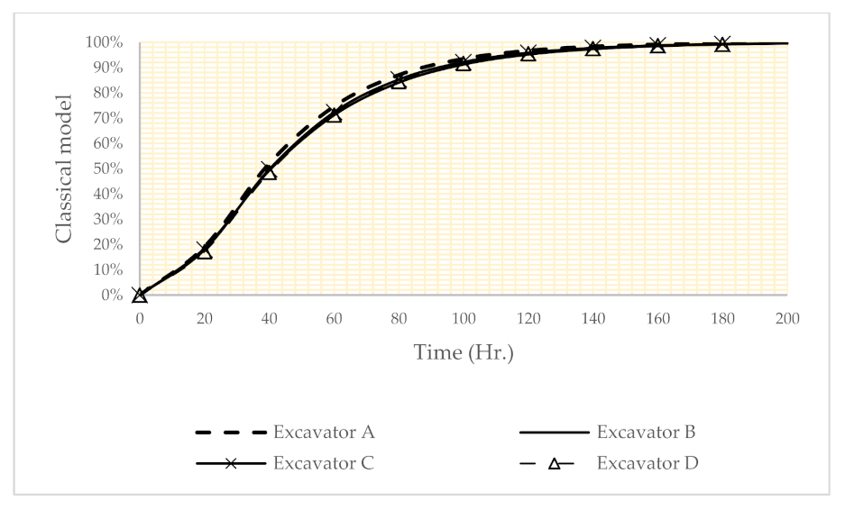
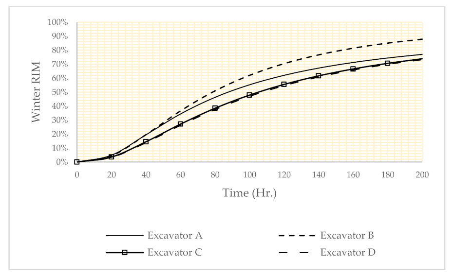
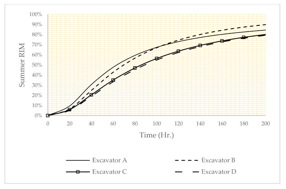
Using Equation (8), the importance measure of the subsystem can be calculated. The result of such analysis is shown in Figure 6, Figure 7 and Figure 8. According to these figures, the importance of the subsystems is dependent on the operational conditions. For example, in Figure 6, the classical model shows that all components have about the same criticality. In the risk factor setting for winter (Figure 7), excavator B has maximum importance measure (first ranking), so excavator B is a critical subsystem. In the risk factor setting for summer (Figure 8), excavator D has the maximum importance measure (first ranking).

Excavator A has the highest reliability (see Figure 4), and its reliability importance is ranked as the lowest importance. The result of the analysis provided that as the importance of the component is changing over time, the resource allocation needs to have a dynamic nature as well, and they need to be updated. For example, the maintenance program needs to be updated as operational conditions are changing.

Table 9. The priority ranking of components in 200 h operation time.

Priority	Condition	Time
		0–20	20–40	40–60	60–80	80–100	100–200
First	Classical Model	D	D	D	D	D	D
	Winter	D	B	B	B	B	B
	Summer	D	D	D	D	D	B
Second	Classical Model	B	C	C	C	C	C
	Winter	B	A	A	A	A	A
	Summer	B	B	B	B	B	A

shows how the reliability importance of the subsystem is changing by operational condition and operating time. For example, in the wintertime, excavator D is the priority. However, after 20 h, excavator B will be the priority.

4. Conclusions

Society’s performance and well-being greatly rely on its infrastructures such as communication, transportation, power distribution. These systems are complex, large, and expensive, often working in dynamic environmental conditions. Resilience is an emerging concept that has been used to quantify the performance of infrastructures. Different concepts have been used to model the resilience of a system, such as reliability and recoverability. To have an effective resilience estimation, the effect of the dynamic operational condition needs to be modeled on the resilience concepts.

Moreover, it is important to know the importance of each component in such complex systems that build up the system. Such a ranking will be based on further improvement and resource allocation. However, in most of the available importance measures, the effect of risk factors has not been addressed properly. For this aim, this paper has introduced a risk factor-based importance measure. The developed model enables the analyst to isolate the observable and unobservable risk factors on the reliability importance of components. Moreover, it developed a step-by-step guideline to facilitate the application of the models.

In this case, the importance of loading fleet number 1 at Gol-Gohar iron ore mine, including four excavators working in parallel, was analyzed in three risk factor sets. The results showed that the system has various important measures in different operating conditions. Moreover, it showed that unobservable risk factors significantly affect the reliability importance of some components. Hence, ignoring these effects may lead to unrealistic decisions.

References

1. Haimes, Y.Y. On the Definition of Resilience in Systems. Risk Anal. Int. J. 2009, 29, 498–501. [Google Scholar] [CrossRef]
2. Barabadi, A.; Ghiasi, M.H.; Nouri Qarahasanlou, A.; Mottahedi, A. A Holistic View on Medical Infrastructures Resilience Before and After COVID-19. Arch. Bone Jt. Surg. 2020, 8, 262–269. [Google Scholar] [CrossRef]
3. Ali, N.G.; Reza, K.; Mohammad, A.; Ashkan, M. Power Law Model for Reliability Analysis of Crusher System in Khoy Cement Factory. In Proceedings of the CIVILICA, 2015, Istanbul, Turkey, 21 July 2015. [Google Scholar]
4. Nouri Qarahasanlou, A.; Barabadi, A.; Ataei, M.; Einian, V. Spare Part Requirement Prediction under Different Maintenance Strategies. Int. J. Min. Reclam. Environ. 2019, 33, 169–182. [Google Scholar] [CrossRef]
5. Lange, D.; Honfi, D.; Theocharidou, M.; Giannopoulos, G.; Reitan, N.K.; Storesund, K. Incorporation of Resilience Assessment in Critical Infrastructure Risk Assessment Frameworks; CRC Press/Balkema: Boca Raton, FL, USA, 2017; pp. 1031–1038. [Google Scholar]
6. Hoseinie, S.H.; Heydari, S.; Ghodrati, B.; Kumar, U. Resilience Measurement of Longwall Machinery. Rud.-Geološko-Naft. Zb. 2020, 35, 39–44. [Google Scholar]
7. Hariri-Ardebili, M.A. Risk, Reliability, Resilience (R3) and beyond in Dam Engineering: A State-of-the-Art Review. Int. J. Disaster Risk Reduct. 2018, 31, 806–831. [Google Scholar] [CrossRef]
8. Gu, Y.; Fu, X.; Liu, Z.; Xu, X.; Chen, A. Performance of Transportation Network under Perturbations: Reliability, Vulnerability, and Resilience. Transp. Res. Part E Logist. Transp. Rev. 2020, 133, 101809. [Google Scholar] [CrossRef]
9. Salomon, J.; Broggi, M.; Kruse, S.; Weber, S.; Beer, M. Resilience Decision-Making for Complex Systems. ASCE-ASME J. Risk Uncert. Engrg. Sys. Part. B Mech. Engrg. 2020, 6, 1–11. [Google Scholar] [CrossRef]
10. Yarveisy, R.; Gao, C.; Khan, F. A Simple yet Robust Resilience Assessment Metrics. Reliab. Eng. Syst. Saf. 2020, 197, 106810. [Google Scholar] [CrossRef]
11. Mottahedi, A.; Sereshki, F.; Ataei, M.; Nouri Qarahasanlou, A.; Barabadi, A. The Resilience of Critical Infrastructure Systems: A Systematic Literature Review. Energies 2021, 14, 1571. [Google Scholar] [CrossRef]
12. Qarahasanlou, A.N.; Khalokakaie, R.; Ataei, M.; Ghodrati, B. Operating Environment-Based Availability Importance Measures for Mining Equipment (Case Study: Sungun Copper Mine). J. Fail. Anal. Prev. 2017, 17, 56–67. [Google Scholar] [CrossRef]
13. Birnbaum, Z.W. On the Importance of Different Components in a Multicomponent System; DTIC Document; Washington Univ Seattle Lab of Statistical Research: Seattle, WA, USA, 1968. [Google Scholar]
14. Chang, H.-W.; Chen, R.-J.; Hwang, F.K. The Structural Birnbaum Importance of Consecutive-k Systems. J. Comb. Optim. 2002, 6, 183–197. [Google Scholar] [CrossRef]
15. Amrutkar, K.P.; Kamalja, K.K. An Overview of Various Importance Measures of Reliability System. Int. J. Math. Eng. Manag. Sci. 2017, 2, 150–171. [Google Scholar] [CrossRef]
16. Almoghathawi, Y.; Barker, K. Component Importance Measures for Interdependent Infrastructure Network Resilience. Comput. Ind. Eng. 2019, 133, 153–164. [Google Scholar] [CrossRef]
17. Chacko, V.M. New Joint Importance Measures for Multistate Systems. Int. J. Stat. Reliab. Eng. 2020, 7, 140–148. [Google Scholar]
18. Xu, A.; Zhang, Z.; Zhang, H.; Wang, H.; Zhang, M.; Chen, S.; Ma, Y.; Dong, X. Research on Time-Dependent Component Importance Measures Considering State Duration and Common Cause Failure. Front. Energy Res. 2020, 8, 259. [Google Scholar] [CrossRef]
19. Kamra, R.; Pahuja, G. Reliability Importance Measures-Based Analysis of Substation Communication Network. In Computational Methodologies for Electrical and Electronics Engineers; IGI Global: Hershey, PA, USA, 2021; pp. 48–66. [Google Scholar]
20. Niu, M.; Xu, N.Z.; Kong, X.; Ngin, H.T.; Ge, Y.Y.; Liu, J.S.; Liu, Y.T. Reliability Importance of Renewable Energy Sources to Overall Generating Systems. IEEE Access 2021, 9, 20450–20459. [Google Scholar] [CrossRef]
21. Zaki, R.; Barabadi, A.; Qarahasanlou, A.N.; Garmabaki, A. A Mixture Frailty Model for Maintainability Analysis of Mechanical Components: A Case Study. Int. J. Syst. Assur. Eng. Manag. 2019, 10, 1646–1653. [Google Scholar] [CrossRef] [Green Version]
22. Rod, B.; Barabadi, A.; Naseri, M. Recoverability Modeling of Power Distribution Systems Using Accelerated Life Models: Case of Power Cut Due to Extreme Weather Events in Norway. J. Manag. Eng. 2020, 36, 05020012. [Google Scholar] [CrossRef]
23. Ghomghale, A.; Ataei, M.; Khalokakaie, R.; Barabadi, A.; Nouri Qarahasanlou, A. The Application of Frailty Model in Remaining Useful Life Estimation (Case Study: Sungun Copper Mine’s Loading System). J. Modeling Eng. 2020, 18, 129–142. [Google Scholar] [CrossRef]
24. Barabadi, R.; Ataei, M.; Khalokakaie, R.; Nouri Qarahasanlou, A. Spare-Part Management in a Heterogeneous Environment. PLoS ONE 2021, 16, e0247650. [Google Scholar] [CrossRef]
25. Barabadi, A.; Barabady, J.; Markeset, T. Maintainability Analysis Considering Time-Dependent and Time-Independent Covariates. Reliab. Eng. Syst. Saf. 2011, 96, 210–217. [Google Scholar] [CrossRef]
26. Barabadi, R.; Ataei, M.; Khalokakaie, R.; Nouri Qarahasanlou, A. Observed and Un-Observed Covariate Effects on Baseline Hazard Rate-Case Study: Jajarm Bauxite Mine. J. Modeling Eng. 2019, 0. [Google Scholar] [CrossRef]
27. Allahkarami, Z.; Sayadi, A.R.; Ghodrati, B. Identifying the Mixed Effects of Unobserved and Observed Risk Factors on the Reliability of Mining Hauling System. Int. J. Syst. Assur. Eng. Manag. 2021, 12, 281–289. [Google Scholar] [CrossRef]
28. Barabady, J.; Kumar, U. Availability Allocation through Importance Measures. Int. J. Qual. Reliab. Manag. 2007, 24, 643–657. [Google Scholar] [CrossRef] [Green Version]
29. Signoret, J.-P.; Leroy, A. Critical States and Importance Factors. In Springer Series in Reliability Engineering; Springer: Berlin/Heidelberg, Germany, 2021; pp. 333–371. [Google Scholar]
30. Dui, H.; Zheng, X.; Guo, J.; Xiao, H. Importance Measure-Based Resilience Analysis of a Wind Power Generation System. Proc. Inst. Mech. Eng. Part O J. Risk Reliab. 2021, 1–11. [Google Scholar] [CrossRef]
31. Zaki, R.; Barabadi, A.; Barabadi, J.; Qarahasanlou, A.N. Observed and Unobserved Heterogeneity in Failure Data Analysis. J. Risk Reliab. 2021, 1–14. [Google Scholar] [CrossRef]
32. Youn, B.D.; Hu, C.; Wang, P. Resilience-Driven System Design of Complex Engineered Systems. J. Mech. Des. 2011, 133, 101011. [Google Scholar] [CrossRef]
33. Hu, Z.; Mahadevan, S. Resilience Assessment Based on Time-Dependent System Reliability Analysis. J. Mech. Des. 2016, 138, 111404. [Google Scholar] [CrossRef]
34. Asha, G.; Raja, A.V.; Ravishanker, N. Reliability Modelling Incorporating Load Share and Frailty. Appl. Stoch. Models Bus. Ind. 2018, 34, 206–223. [Google Scholar] [CrossRef]
35. Xu, M.; Li, X. Negative Dependence in Frailty Models. J. Stat. Plan. Inference 2008, 138, 1433–1441. [Google Scholar] [CrossRef]
36. Misra, N.; Gupta, N.; Gupta, R.D. Stochastic Comparisons of Multivariate Frailty Models. J. Stat. Plan. Inference 2009, 139, 2084–2090. [Google Scholar] [CrossRef]
37. Giorgio, M.; Guida, M.; Pulcini, G. Repairable System Analysis in Presence of Covariates and Random Effects. Reliab. Eng. Syst. Saf. 2014, 131, 271–281. [Google Scholar] [CrossRef]
38. Barker, K.; Baroud, H. Proportional Hazards Models of Infrastructure System Recovery. Reliab. Eng. Syst. Saf. 2014, 124, 201–206. [Google Scholar] [CrossRef]
39. Mottahedi, A.; Sereshki, F.; Ataei, M.; Qarahasanlou, A.N.; Barabadi, A. Resilience Analysis: A Formulation to Model Risk Factors on Complex System Resilience. Int. J. Syst. Assur. Eng. Manag. 2021, 12, 871–883. [Google Scholar] [CrossRef]
40. Rød, B.; Barabadi, A.; Gudmestad, O.T. Characteristics of Arctic Infrastructure Resilience: Application of Expert Judgement. In Proceedings of The 26th International Ocean and Polar Engineering Conference, Rhodes, Greece, 26 June–1 July 2016. [Google Scholar]
41. Gutierrez, R.G. Parametric Frailty and Shared Frailty Survival Models. Stata J. 2002, 2, 22–44. [Google Scholar] [CrossRef] [Green Version]
42. Kumar, D.; Klefsjö, B. Proportional Hazards Model: A Review. Reliab. Eng. Syst. Saf. 1994, 44, 177–188. [Google Scholar] [CrossRef]
43. Schoenfeld, D. Chi-Squared Goodness-of-Fit Tests for the Proportional Hazards Regression Model. Biometrika 1980, 67, 145–153. [Google Scholar] [CrossRef]
44. Park, S.; Hendry, D.J. Reassessing Schoenfeld Residual Tests of Proportional Hazards in Political Science Event History Analyses. Am. J. Political Sci. 2015, 59, 1072–1087. [Google Scholar] [CrossRef] [Green Version]
45. Brewer, M.J.; Butler, A.; Cooksley, S.L. The Relative Performance of AIC, AICC and BIC in the Presence of Unobserved Heterogeneity. Methods Ecol. Evol. 2016, 7, 679–692. [Google Scholar] [CrossRef]
46. Kuha, J. AIC and BIC: Comparisons of Assumptions and Performance. Sociol. Methods Res. 2004, 33, 188–229. [Google Scholar] [CrossRef]
47. Garmabaki, A.H.S.; Ahmadi, A.; Mahmood, Y.A.; Barabadi, A. Reliability Modelling of Multiple Repairable Units. Qual. Reliab. Eng. Int. 2016, 32, 2329–2343. [Google Scholar] [CrossRef]
Figure 1. Resilience concept [11].
Energies 14 07575 g001
Figure 2. The framework proposed for risk factor-based reliability importance measure (RF-RIM).
Energies 14 07575 g002
Figure 3. A framework for the reliability model [31].
Energies 14 07575 g003
Figure 4. Subsystem reliability for risk factors: temperature = 20, afternoon shift, ore and operation team B.
Energies 14 07575 g004
Figure 5. System reliability under three different risk factor settings.
Energies 14 07575 g005
Figure 6. The results reliability importance measure in the classical model reliability.
Energies 14 07575 g006
Figure 7. The results reliability importance measure in the winter reliability.
Energies 14 07575 g007
Figure 8. The results reliability importance measure in the summer reliability.
Energies 14 07575 g008