Article

Verification and Validation of Large Eddy Simulation for Tip Clearance Vortex Cavitating Flow in a Waterjet Pump

1
State Key Lab of Water Resources and Hydropower Engineering Science, Wuhan University, Wuhan 430072, China
2
Wuhan Second Ship Design and Research Institute, Wuhan 430064, China
*
Author to whom correspondence should be addressed.
Energies 2021, 14(22), 7635; https://doi.org/10.3390/en14227635
Submission received: 25 September 2021 / Revised: 5 November 2021 / Accepted: 9 November 2021 / Published: 15 November 2021
(This article belongs to the Special Issue Advances in Pumped Storage Hydraulic System)

Abstract

:
In this paper, large eddy simulation (LES) was adopted to simulate the cavitating flow in a waterjet pump with emphasis on the tip clearance flow. The numerical results agree well with the experimental observations, which indicates that the LES method can make good predictions of the unsteady cavitating flows around a rotor blade. The LES verification and validation (LES V&V) analysis was used to reveal the influence of cavitation on the flow structures. It can be found that the LES errors in cavitating region are larger than those in the non-cavitating area, which is mainly caused by more complicated cavitating and tip clearance flow structures. Further analysis of the interaction between the cavitating and vortex flow by the relative vorticity transport equation shows that the stretching, dilatation and baroclinic torque terms have major effects on the generation and transport of vortex structure. Meanwhile the Coriolis force term and viscosity term also exacerbate the vorticity transport in the cavitating region. In addition, the flow loss characteristics of this pump are also revealed by the entropy production theory. It is indicated that the tip clearance flow and trailing edge wake flow cause the viscous dissipation and turbulent dissipation, and the cavitation can further enhance the instability of the flow field in the tip clearance.

Graphical Abstract

1. Introduction

Tip clearance exists widely in various kinds of turbomachines to avoid striking between the impeller and casing wall. However, the tip leakage vortex (TLV) flow through the rotor-shroud gap will unavoidably cause a performance penalty and flow loss [1]. Moreover, the vortex structures and multiple complex re-entrant flows may raise numerous issues in rotors [2]. A prominent matter is the cavitation phenomenon, which can influence the pump hydrodynamic performance, bring about a reduction in stability for turbines and cause power output ability reduction, noise and vibration [3]. Cavitation in the waterjet pump has always been an area of particular interest in cavitating flow study for many years owing to the tip clearance and complicated flow mechanisms.
The TLV is apt to cause vortex cavitation around the rotor-shroud clearance [4,5]. A single hydrofoil with tip clearance can be considered as a special example to study the TLV cavitation. But the relative motion caused by the impeller and the casing wall in an actual pump is difficult to describe with a single static part [6,7,8]. Even though the highly twisted blades and numerous complex vortices inside the pump make it extremely difficult to measure the data around the tip clearance, many researchers still strive to obtain the data about vortex and cavitation [9,10]. Additionally, the computational fluid dynamics (CFD) technique serves as a powerful tool for researchers to solve cavitation problems in engineering [11]. The development of numerical simulation technology has promoted the research process of vortex and cavitation flow in hydraulic machinery. It is of great significance to study the characteristics of vertical flow, cavitation evolution, the interaction of cavitation and vertical structure, and pressure pulsation. Among the various turbulence models, the Shear-Stress-Transport (SST) model has good performance in capturing vertical structures such as TLV [10]. In addition to this model, there are other models including k-ε, renormalization group k-ε (RNG) and the reynolds stress model (RNG) model; they have also been adopted for the prediction of hydrodynamic performance and cavitation in rotating machinery, but they still could not yield more accurate numerical results in some complex cases [12].
Although numerical simulation technique has improved recently, most investigations are still limited to predict the cavitation patterns and TLV trajectory. The above-mentioned research investigations on the effects of cavitation and TLV on the flow characteristic had difficulty to meet the requirements of large eddy simulation (LES), owing to the rigorous grid resolution and computational requirements. LES has been tentatively used for fundamental cavitation investigations, and it is also a prospective method to improve prediction accuracy and cavitating flow research in waterjet pump. You et al. [13] applied the LES method to predict tip-leakage cavitating flows in a turbomachinery cascade with emphasis on the potential mechanisms for viscous losses nearby the tip clearance. Shen et al. [14] used LES to simulate unsteady tip leakage flows in an axial flow pump; the results revealed the influence of different gap sizes on the internal flow field of the pump. Li et al. [15,16] also showed the effect of the clearance size on the leakage flow and the pressure fluctuation. The LES method has achieved good application results in the study of water jet pump cavitation, but owing to the high demand on grid resolution and expensive computing consumption, such investigations are still rare, especially quantitative analysis. Therefore, it is meaningful to carry out some quantitative LES research.
Although the reliability and exactness of the LES has been broadly approved in numerous studies, the quantitative evaluation of its precision is still insufficient in the previous literature. Grid independence verification and reliability studies are mainly verified by contrasting with visual snapshots. Many of the strict research efforts were insufficent in their ability to quantitatively assess the precision of LES. Results about the precision of LES are crucial to verify the dependability of simulation results for complicated cavitating cases, when there is insufficient measured data to confirm the calculation results. The Direct Numerical Simulation (DNS) method and experiments are usually used as verification benchmarks for some cases, but their huge costs are unbearable for engineering applications. Moreover, the LES method is used to model the complex flow features. If it needs to be verified by experiments every time, then the numerical method for prediction will be meaningless. Therefore, a quantitative evaluation method—Verification and validation (V&V) —can be applied for LES numerical calculation and independent of experiments [17,18]. The method is a mathematical way to evaluate a physical model’s precision and computational result accuracy [19,20]. V&V is defined by the American Society of Mechanical Engineers: verification represents accuracy of the numerical solution procedure and validation is used to indicate that the constructed physical model can accurately reflect the real physical phenomena and rules. The LES V&V is different from the RANS V&V [20]; LES V&V is a more significant but harder problem needing additional exploration. Freitag, Klein [19,21] and Xing [22] raised some new ways for evaluating LES errors from a mathematical point of view, and one of these methods was refined by Dutta and Xing [23,24], thus providing an important foundation for promoting LES V&V research. Recent studies by Long et al. [25,26] put the LES V&V method into cavitating flows around a propeller and a hydrofoil [27]. This paper further makes use of LES V&V method for the analysis of the complex cavitating flow inside the waterjet pump.
The purpose of this investigation is to discuss the effect of cavitation on the flow field in a waterjet pump by the LES V&V method, with emphasis on the tip clearance flow. A referenced experiment in this waterjet pump is applied to validate the numerical data. The LES V&V method with simplified three-equations is employed in the investigation of tip clearance cavitation. The features of LES errors and the effects of cavitation on the total errors are analyzed by three sets of refined structured mesh. Furthermore, the impact of cavitation on the vorticity distributions and the flow loss features are discussed.

2. Governing Equations

The tiny time step size and extremely fine grid are responsible for the enormous computation cost in solving the Navier-Stokes equations (N-S equations) with the DNS method. For that reason, the LES method was proposed to greatly reduce computing consumption through a low-pass filtering of the N-S equations, which eases the requirement of time step size and grid.
In the homogeneous model frame for vapor and liquid flows, the same turbulence flow field for the multiphase components is assumed. The basic governing equations, including the mass and momentum conservation equations are written as:
ρ m t + ( ρ m u j ) x j = 0
( ρ m u i ) t + ( ρ m u i u j ) x j = p x i + x j ( μ m u i x j )
where p is the mixture pressure, and ui is the mixture velocity component in the i direction. The laminar viscosity of mixture, μm, and the mixture density, ρm, are defined as:
μ m = α v μ v + ( 1 α v ) μ l
ρ m = α v ρ v + ( 1 α v ) ρ l
where the subscript l represents liquid and v denotes the vapor phase. The LES equations can be obtained by performing a Favre-filtering operation to Equations (1) and (2):
ρ m t + ( ρ m u ¯ j ) x j = 0
( ρ m u ¯ i ) t + ( ρ m u i ¯ u j ¯ ) x j = p ¯ x i + x j ( μ m u ¯ i x j ) τ ij x j
where the over-bars represent filtered quantities. The extra non-linear term in Equation (6) is called the subgrid-scale stresses (SGS stresses); those stresses occur due to the filtering operation, and need to be modeled and is defined as:
τ ij = ρ ( u i u j ¯ u i ¯ u j ¯ )
To calculate the SGS stresses, an eddy viscosity method is applied by scaling the strain rate tensor, S ij ¯ , as:
τ ij 1 3 τ kk δ ij = 2 μ t S ij ¯
S ij ¯ = 1 2 ( u i ¯ x j + u j ¯ x i )
where τkk represents the isotropic term of the SGS model, and μt is the SGS turbulence viscosity, which is closed by the Wall Adapting Local Eddy-Viscosity (WALE) model.
μ t = ρ L s 2 ( S ij d S ij d ) 3 / 2 ( S ij S ij ¯ ) 5 / 2 + ( S ij d S ij d ) 5 / 4
L s = min ( κ d , C w V 1 / 3 )
S ij d = 1 2 ( g ij ¯ 2 + g ji ¯ 2 ) 1 3 δ ij g kk ¯ 2 , g ij ¯ = u i ¯ x j
where κ is the von Karman’s constant, d is the distance to the nearest wall, Cw is the WALE constant with the default value of 0.5, and V is the computational cell volume. Compared with the Smagorinsky-Lilly model [28], the WALE model shows better performance in recreating the laminar to turbulence transition with the requirement of the near-wall distance y3 law [29].
The transport equation with the homogeneous hypothesis is employed to simulate multiphase flow, and both two phases, liquid and vapor phases, are considered as incompressible phases [30,31,32]. The Zwart cavitation model [31] is one of the widely used models in many solvers for cavitating flow, whose accuracy has obtained wide approval [5,32]. The cavitation process is described by the following vapor transfer equation:
( ρ v α v ) t + ( ρ v α v u j ) x j = m ˙ + m ˙
The source terms m ˙ + and m ˙ in Equation (13) are derived from the simplified Rayleigh–Plesset equation and represent the vaporization and condensation rates, respectively, which are expressed as:
m ˙ + = F vap 3 α nuc ( 1 α v ) ρ v R 2 3 | p v p | ρ l
m ˙ = F cond 3 α v ρ v R 2 3 | p v p | ρ l
The model coefficients are,
R = 1 × 10 6 m
α nuc = 5 × 10 4
F vap = 50
F cond = 0 . 01
These constants are recommended by Zwart et al. [31] and are recognized in the study of cavitation characteristics.

3. Application of V&V Approach in Waterjet Pump

The V&V approach [33,34] of LES has been applied in the research field of hydrofoil cavitation, which can also be generalized to cavitating flow field around rotating machineries [35]. The paper mainly analyzes the flow field through the error distribution obtained by the LES V&V. The error obtained by numerical calculation can be divided into two parts, namely modeling error and numerical error [25,27]. The numerical error is introduced by the SGS model and the modeling error is determined by the by grid and numerical accuracy. In most cases, these two parts of error have different signs in the case, which means that the total error may be small. In this paper, the absolute value of the two errors is chosen to observe the change law intuitively. However, the exact solution is always hard to obtain for the cavitation case, so the numerical benchmark is regarded as the exact solution. The numerical benchmark represents the high-precision computational result and it can be approved by most investigators. The two parts of error deduced from the V&V approach of LES can be denoted as:
S S C = c N ( h ) p N + c M Δ p M
h = Δ t × Δ N
where S is the value of a variable obtained by calculation, and SC represents the numerical benchmark. The two terms on the right-hand side of Equation (16) signify the numerical error and the modeling error, respectively, in which cN and cM represent the coefficients of the two kinds of errors, pN and pM are the accuracy orders of the two errors. ∆t is the time step and ∆N is the local grid size. As for the procedure proposed by Long et al. [35], the three-equation method is normally suitable for the rotating machine calculation and the recommended reference values of pN and pM are 1.48 and 1.37, respectively [35]. The present LES V&V method adopts three systematically refined grids with unsteady computations solving for the three variables (SC, cN and cM):
S 1 S C = c N ( h ) p N + c M Δ p M
S 2 S C = c N ( r h ) p N + c M ( r Δ ) p M
S 3 S C = c N ( r 2 h ) p N + c M ( r 2 Δ ) p M
where S1, S2 and S3 are solutions of a variable calculated by the three sets of mesh, r is the grid refinement ratio and also the time-step rate of change and r = 1.2 is usually used to solve the three non-linear and complicated equations. Eventually, only three transient solutions by three sets of grids are required to obtain the two parts of error.
Three systematically refined grids are generated for the waterjet pump to calculate the transient results, as shown in Table 1. The velocity is regarded as the target variable to solve the three complex non-linear equations, Equations (18)–(20). Then, the LES errors can be obtained.
In summary, based on the previous research [20,23,25,36] on LES V&V, the value of r between 1 and 2 is more appropriate. Too large a value of r will make the computation capacity insufficient, while a smaller ratio will make it difficult to distinguish the LES and iteration errors. Most notably, the iteration error in the solution process of the investigation is much smaller than the error of LES, so that the iteration error can be ignored. Therefore, in consideration of the current calculation capacity, a reasonable refinement ratio r = 1.2 is chosen in present study.

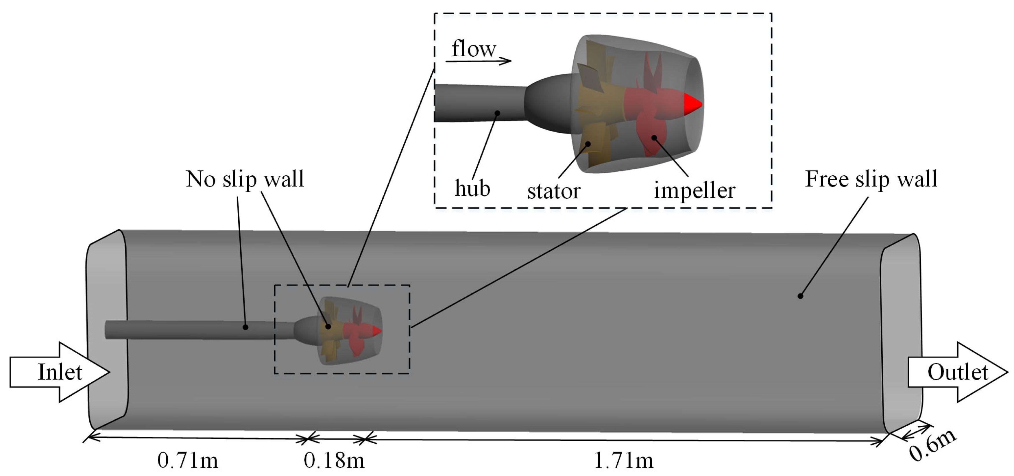
4. Waterjet Pump Geometry, Numerical Setup and Mesh Information

Figure 1 shows the geometry of the waterjet pump. The rotor blade number is six, and the stator number is eight. The computational domain used in this paper is consistent with the experiment, as shown in Figure 1 The entire computational domain is composed of the stator domain, the impeller domain and the outer domain, and these parts of the computational domain are connected by a general grid interface (GGI) technology. This method has been proved to be effective to weigh the prediction exactness and calculation consumption [32,35,37,38,39,40]. All the surfaces of the waterjet pump, including the impeller, stator, pump casing wall and shaft surface are all set as no-slip wall conditions. The free-slip wall condition is set for the external flow channel surface. The computational domain size and operating condition are consistent with the experiment.
TLV is mainly generated in the gap area, so improving the grid accuracy in the tip clearance is of great significance to improve the prediction accuracy of the vortex structure [25]. Special attention should be paid when constructing high-quality meshes in this paper, particularly in the clearance region. The structured grid was applied in the entire computational domain, which has the advantages of better convergence and more reduction of truncation error. The mesh distribution is shown in Figure 2.
Usually, the calculation of unsteady cavitating flow is based on the simulation convergence results under non-cavitating conditions to ensure the convergence speed. When the root mean square (RMS) residual criterion was lower than 10−6, the non-cavitation result was considered to be convergent and stable. During the transient cavitation calculation, the transient rotor stator method was used for the interface setup. The high resolution scheme [41,42] was solved by the convection terms and the transient term adopted the second order backward Euler scheme. Taking into account the calculation accuracy and calculation time cost, the number of inner iteration steps used in the calculation was 20 steps per time step, and the residual convergence standard was 10−5. All unsteady computations for each set of grids ran over 25 impeller revolutions, with the final results obtained over the last 10 impeller revolutions. The inlet velocity was U = 2.496 m/s corresponding to the experiment measurement and the outlet static pressure condition was obtained from the cavitation number σ = (poutpv)/(0.5ρn2D2) = 2. The impeller diameter D was 166.4 mm and the rotational speed n was 1500 rpm.

5. Results and Discussions

5.1. Hydrodynamic Performance for the Pump

The experiment and calculation results for the hydrodynamic performance of the pump are presented in Figure 3. The experimental data is the same as the work done by Han [43]. In Figure 3, the abscissa represents the advance ratio, J = V/nD, and the ordinate represents two dimensionless hydrodynamic performance parameters, namely the thrust coefficient (KT = thrust/ρln2D4) and the torque coefficient (KQ = torque/ρln2D5). The predicted results are highly consistent with the measured data and the errors in the calculation of KT and KQ are less than 5% over the wide range of the advance coefficient J, thereby it indicates that the present computational methods are capable of simulating the pump hydrodynamic performance well. Furthermore, the close proximity of predicted results by three meshes indicates that grid resolution has little effect on the numerical results.

5.2. Unsteady Cavitation of the Experimental and Numerical Results

The predicted transient cavitation and vortex snapshots as the impeller rotates at a certain moment are shown in Figure 4. The spatial cavitation shapes vortex structures are presented by the iso-surface of vapor volume fraction αv = 0.1 and the iso-surface of Q criterion in the predicted results, respectively. The cavitation patterns for the waterjet pump are completely captured by LES for all three sets of grids. Since the low pressure area is mainly concentrated in the tip clearance position, cavitation is easily generated at the tip of the blade and quickly extends to the entire tip. At the same time, the TLV cavitation begins to generate as the blade rotates. The tip clearance cavitation swings as it is drawn into the TLV. Then, the cavitation shapes remain basically stable as the blade rotates.
By comparing the predicted and observed cavitation for the pump, the TLV cavitation has developed in the snapshot as shown in Figure 4 and is very strong. As the rotor blade rotates, the TLV cavitation slightly swings and the trailing of the cavitation becomes unstable. All three meshes clearly show the entire cavitation patterns and the tip clearance cavitation and TLV cavitation are all similar. With the gradual increase of the grid number, there are only a few subtle differences at the tail of vortex cavitation TLV—the length between the calculation results of different grids (marked by a red line). The overall cavitation patterns around all blades are relatively similar, and achieve a strong agreement with the experiment results. From the iso-surface of the Q criterion, it can be seen that the vortex structure is enriched with the increase of the number of grids, and the ability to capture the vortex structure, such as the induced vortex and leakage vortex around the impeller, was significantly improved.
As the cavity is made up of vapor, Figure 5 displays the distribution of vapor around the blade tip. The contour map in Figure 5 shows the cavitation by selecting the sections at two different radiuses r/R of the clearance area, where r represents the selected radius position, and R represents the radius of the pump casing. In Figure 5b, the plane is arranged between the blade tip and the pump casing, and the cavitation area presents a triangular shape with an angle of 83 degrees to the axial direction. The referenced measured data has proved that this angle would remain constant with the further change of cavitation number [10]. In Figure 5a, the section position is slightly away from the casing wall, the blank areas in the contour represent the cross-section of blades. In Figure 5a, it can be found that the TLV cavitation gradually separates from the tip area and extends downstream. Therefore, a certain angle is formed by TLV cavitation and tip clearance cavitation, which leads to the formation of a triangular cavitation region. A higher volume of the cavity is concentrated around the blade suction side and it collapses and disappears rapidly near the trailing edge and downstream.
The transient flow phenomenon of the tip clearance cavitation and the TLV cavitation as the pump impeller runs is reproduced excellently by the present LES computational method. These results show the high performance prediction fidelity and the great computational capability with the combination of the structured mesh and the LES method used in this study. At the same time, in order to balance the calculation pressure and accuracy, Mesh 2 is already sufficient to meet the requirements.

5.3. V&V Results of LES for the Tip Clearance Cavitating Flow in the Pump

The former section mainly verified the feasibility of the calculation method and the independence of the grid through the comparison of macroscopic physical observations and simulated results, but these qualitative analyses do not provide a quantitative assessment. Therefore, this section applied the V&V method of LES based on the three-equation model to illustrate the characteristics of the flow field from a mathematical point of view. It is noteworthy that all predicted cavitation patterns in the previous section are the instantaneous results. In this section, however, the time-averaged velocity from each transient result over all monitoring points around impeller blades is used for LES V&V analysis.
Figure 6 and Figure 7 mainly show the position of the monitoring points and the relationship between cavitation phenomenon and the LES error. In Figure 6a, the monitoring points in Region A (P1 to P5) denote the locations in the clearance between the tip and casing wall, and the points in Region B (P6 to P10) mainly represent positions in the TLV cavitation area. The monitoring points in Region C (P11 to P13) represent positions in the downstream area of the blade trailing edge. P14 to P16 are located immediately behind the tip vortex cavitation. Figure 6b shows the relative position between the cavitation and the monitoring points, and it should be noted that P2 to P10 are located inside the cavity. The calculated LES errors based on the average velocities at these monitoring points are shown in Figure 7b,c. The standard deviations of velocity are also used to reveal the dispersion level of the velocity results [43].
As shown in Figure 7a, the standard deviation fluctuates in Region A. This parameter first rises slightly, then falls, and finally rises to a larger value. Among them, there is the maximum value at P2 and the minimum at P4. The severe tip clearance flow and cavitation inception cause a larger level at P2. From P6 to P8, the standard deviation increases substantially and the reading reaches the maximum at P10. The velocity fluctuation is limited in the passageway region between two blades, so the standard deviations at P6 and P7 are at a low level. The velocity variety at P8 is most affected by the strong cavitation and wake flow caused by the blade trailing edge, and the standard deviation at P10 is influenced by the TLV cavitation and tip clearance flow from the next blade. The standard deviations in Region C and Region D are all relatively small, and the value in Region D is smallest. These phenomena can be reasonably explained in combination with the tip clearance flow and cavitating flow shown in Figure 7b. The monitoring points with large standard deviation readings are mainly concentrated in the gap flow area and the cavitation area. The standard deviation readings far away from the tip clearance cavitation zone and the blade wake zone are all small, which indicates that the flow stability is greatly affected by the unsteady clearance cavitation and wake flow (P2 and P5 above the tip in Region A, P8 near the wake region and P10 near the next blade tip clearance).
The distributions of LES errors have some differences with the standard deviation. The variation trend of the LES error in Region A is more consistent with that of standard deviation. The peak values occur at P2 and P5. The overall amplitude of the LES error in Region B is relatively similar, and the amplitude is the largest at the point P6, and then the errors at points P7 to P10 fluctuate in a small range. In Region C, the readings at P11 to P12 are small and then rise slightly at P13. For points P14 to P16 in Region D, all values are at a low level.
In order to more clearly explain the connection between the LES errors and the tip clearance cavitation flow, the error distribution of the monitoring points P1 to P5 and P14 to P16 corresponds to the flow field position in Figure 6b. In the tip gap area (Region A), the error at P1 is most affected by the tip clearance flow, so the LES error is larger in Region A at P1 than in Region D. In the cavitation area (P2 to P5), P2 is located at the point where tip clearance cavitation occurs and collapses. The flow field at this position is significantly affected by the change of cavitation volume, and this point is also significantly affected by the tip clearance flow. The point where the maximum LES error occurs in Region A is the P2 monitoring point. Therefore, it shows that the error distribution of the P2 point can indicate that the position is disturbed by cavitation and gap flow to a certain extent, although the cavitation changes in the position of P3 to P4 are smaller; P3 is closer to the starting point of the TLV, the impact is more obvious, and the resulting LES error is also larger. Point P5 is closer to the trailing edge of the blade than are P3 and P4, and the flow separation effect caused by rotation is more obvious. At the same time, the proximity of P5 to the trailing edge of the blade further reduces the flow stability at this position. These reasons lead to the low flow field stability of P5 and relatively large LES error.
In the downstream region, the rotor influence reduces and the flow complexity becomes weaker at the position further away from the blade tip and cavitation region, so the LES errors decrease remarkably in Region D. However, since the points P6 to P10 are located inside the cavity, the LES errors in Region B are all in the high level. The larger amplitude at P6 is caused by the effects of cavitation and tip clearance flow, but this point is not inside the gap, and the impact is relatively not so strong, while the higher level at P10 is caused by the swing of the TLV cavitation tail.

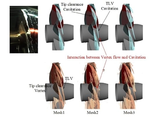
5.4. Effect of Cavitation on the Vortex Distribution in the Pump

The last chapter mainly explained the influence of cavitation and clearance flow on the flow field around the impeller from a quantitative perspective. This part further elaborates the influence of cavitation on the vorticity field in the tip clearance area. All the following results are calculated by the Mesh 2. In order to understand the vorticity distribution in depth, the relative vorticity transport equation is mainly used to discuss the effect of cavitation on the vorticity field. The equation is shown as following [35]:
Ω rel t = ( Ω rel ) U rel Ω rel ( U rel ) + 1 ρ m 2 ρ m × p m 2 × ( ω × U rel ) + υ 2 Ω rel
where Ωrel is the relative vorticity, u is the relative velocity, ν is the kinematic viscosity, ω is the rotor rotational speed, the subscript of rel represents the variable in cylindrical coordinates, and ∇ is the Hamiltonian operator. The left side of Equation (21) is the derivative of the relative vorticity. Each term on the right side represents the relative vortex stretching, relative vortex dilatation, relative baroclinic torque, the Coriolis force terms and viscous diffusion, in turn. Since the velocity gradient will cause the stretching and distortion of the vortex structure, the vortex stretching and tilting term is used to characterize the stretching and distortion of the vortex, which is called the stretching term. The relative vortex dilatation term is mainly used to characterize the volume change of the vapor phase in a multiphase flow. The baroclinic torque term only exists in the baroclinic fluid and is caused by the non-parallelism between the pressure and the density gradient. The Coriolis force term is induced by the rotation effect. The fifth term is the viscous diffusion term that characterizes the effect of viscosity on vorticity transport. In order to show the distribution of the vorticity field around the blade tip more clearly, all pictures in this part display the flow at one typical moment.
Figure 8a shows the specific locations of the six cross-sections around the blade tip. The cavitation structures are displayed by the iso-surfaces of the vapor volume fraction αV = 0.1. The planes mainly correspond to the generation, development and trailing edge of the tip clearance cavitation region.
Figure 8b–i show the distributions of the vapor volume fraction, Q-criterion, relative vorticity and the five terms on the right side of the relative vorticity transport equation that affect vorticity transport for the cavitating flow around the rotor blade tip.
As shown in Figure 8b, the predicted tip gap cavitation and TLV cavitation are generated from the tip and grow around the suction side, and finally form the vortex cavitation downstream. In Figure 8c, the largest magnitude of Q occurs at the vortex cavity core and in the liquid-vapor interface regions and the distributions are in broad agreement with the vapor volume fraction. In addition, the TLV cavitation is relatively short, but TLV is strong enough to extend far downstream.
In Figure 8d, the distribution of relative vorticity is presented around the blade tip region. In the blade tip clearance zone, the relative vorticity is concentrated at the liquid-vapor interface. Significantly, the vorticity inside the tip vortex cavity is larger than that in the other regions. Meanwhile, the highly concentrated vorticity on Planes 1–3 is also associated with the vortex cavitation caused by the previous blade.
As shown in Figure 8e, due to the relative motion between the shroud wall and the rotor blades, there will be a large velocity gradient between the two, which will cause a high relative vorticity distribution. Moreover, because of the effect of complex flow and cavitation on the gap flow field, the peak value of stretching term is largely concentrated around the blade tip cavitation region and trailing edge wake.
Figure 8f shows the distribution of the relative dilatation term. When the fluid volume changes have an effect on the vortex field, the relative expansion term takes effect, and the relevant concentration area is mainly in the vortex cavitation and wedge-shaped cavitation areas. It is worth noting that the effect of the relative dilatation term near the TLV is more significant than that of the tip clearance cavitation.
Figure 8g shows that the relative baroclinic torque term is concentrated in the junction area between the vapor and liquid. This term can reflect the misalignment condition of the pressure and the density gradients, so the distribution of this term is almost concentrated in the cavitation area.
In Figure 8h,i the viscosity term and the Coriolis force term affect a relatively small range mainly near the blade tip and trailing edge wake area. The viscosity term is mainly concentrated around the blade tip clearance and the flow structure scale is small, so the viscous dissipation has a strong effect on the local vorticity distribution. The Coriolis force term mainly characterizes the vorticity transport caused by the rotation effect and the term is apparently affected by the wake of the blade trailing edge.
In previous studies, the vorticity transport equation was used to describe the vorticity distribution around the stationary hydrofoil [44], but the transport characteristics of the vortex field caused by the rotation effect in rotating machinery are obviously more complicated. For one thing, the relative movement of the rotor blades and the shroud wall has a more obvious influence on the surrounding flow field and vorticity field. For another, the tip clearance cavitation on the blade tip influences the vorticity generation near the region. In the meantime, these flow characteristics in the pump have a cavitating flow different from that around a single hydrofoil [45].

5.5. Effects of Cavitating Flow on Entropy Production Characteristics

According to the above analytical discussion of the tip clearance cavitating flow characteristics, it can be found that the flow around the tip of the pump becomes more complicated with the production and development of the cavitation. The tip clearance inevitably becomes an important cause of flow loss [46], and the change of the cavitating flow structure will decrease the flow stability [37], both of which have a non-negligible impact on the operational stability and hydraulic performance of the impeller and even the whole pump. In order to further describe the relationship between cavitation flow and flow loss, the flow loss around the clearance is assessed from the perspective of thermodynamics through the results of numerical calculations in this part, and the association of flow loss distribution and cavitation is revealed by entropy production evaluation method [47,48]. Solving the entropy production equation yields two terms, one with a time-averaged term and one with a fluctuating term [49,50].
S = ( Φ T ) ¯ = S EP D + S EP D ¯
S EP D ¯ = μ T ¯ [ 2 { ( u ¯ x ) 2 + ( v ¯ y ) 2 + ( w ¯ z ) 2 } + ( u ¯ y + v ¯ x ) 2 + ( u ¯ z + w ¯ x ) 2 + ( v ¯ z + w ¯ y ) 2 ]
S EP D = μ T ¯ [ 2 { ( u x ) 2 + ( v y ) 2 + ( w z ) 2 } + ( u y + v x ) 2 + ( u z + w x ) 2 + ( v z + w y ) 2 ]
where u represents the pulsating pressure, u ¯ represents the time-averaged result within the sampling time, μ denotes the dynamic viscosity and T denotes the temperature. The first group denotes entropy production by dissipation in the time-averaged flow field, which is the so-called direct or viscous dissipation term. The second term is then referred to as the indirect or turbulent dissipation.
Figure 9 reveals that the viscous dissipation and turbulent dissipation of the entropy production has a variation relative with the change of tip clearance flow and cavitation. The dominant entropy production is concentrated in the tip clearance cavitation region, which is caused by the high shearing effect. As the investigated operating condition is at a low cavitation number, the formed tip clearance cavitation and TLV cavitation have a relatively violent characteristic and the entropy production features around the blade tip are mainly determined by the cavitation, blade rotation and rotor-shroud interaction. Additionally, the two terms of the entropy production are almost equal to zero in the downstream vortex cavitation core in Plane 1 to 2 and Plane-6, and the larger amplitude appears around the tip clearance cavitating flow region and blade trailing edge wake region.
The viscous dissipation term features on these recording planes reveals the influence of dissipation in the rotational direction. The distribution of the viscous dissipation term around the blade tip region is shown in Figure 9b. As the cavitation extends to downstream, the high viscous dissipation region also migrates to the downstream. On the blade tip, the maximal amplitudes appear around the tip clearance cavitating flow region and the blade trailing edge wake. In Figure 9c, the turbulent dissipation is also fairly obvious near the tip clearance cavitation region. The rotation effect of the blades and the existence of the tip clearance will cause strong flow separation in the tip area, and the complexity of the flow will increase, resulting in higher entropy production. Meanwhile, the emergence of cavitation will further increase the entropy production around the clearance region. The tail of the blade will produce a complex wake vortex structure, which will also cause a higher entropy value. Overall, the variety of the entropy production is mainly determined by the tip clearance flow and blade trailing edge wake flow, and the appearance of cavitation will further deteriorate the stability of the flow and increase the production of entropy.

6. Conclusions

The tip clearance cavitation in a waterjet pump was investigated by numerical simulation. The calculated hydrodynamic performance and the cavitation pattern are mainly compared with the experimental results, and the tip clearance flow and cavitation characteristics in the pump are analyzed mathematically by using the V&V method of LES. The vorticity transport, association between cavitation and tip clearance flow and flow loss were analyzed in the present studies. The results summarized from the above analysis are as follows:
(1)
The hydrodynamic performance and cavitation patterns in the pump can be precisely simulated by LES. Both the cavitation shape and location can be predicted accurately, which is in good agreement with the test. Therefore, the numerical calculation method and the adopted grid and model can be proved to be suitable for simulating the transient cavitating flow in the pump;
(2)
The LES error reflects the flow field around the rotor affected by transient cavitation and tip clearance flow to some extent. The LES errors calculated from the average velocity at the monitoring points inside the cavity are clearly larger than the error in the non-cavitation region. The relatively larger cavity volume variations and more violent collapse of the cavity around the head of the blade tip due to more unsteady tip clearance flow increase the difficultly of numerical calculation. The interaction between cavitation and the tip clearance flow makes the prediction of multiphase flow around a rotor blade tip much harder than that of a pure tip clearance flow;
(3)
The effects of the cavitation on the vorticity field are analyzed by the relative vorticity transport equation. In the cavitation area, the vorticity is mainly concentrated in the TLV cavity core and at the liquid-vapor interface. The vortex stretching term is larger around the blade tip and the dilatation term is centered near the TLV cavitation area. The baroclinic torque term is visible around the cavity interface. The Coriolis force term and viscosity term spread in the blade tip region and trailing edge wake, respectively. It reveals that the cavitation and tip clearance flow make a significant contribution to the vorticity generation and transport;
(4)
The flow loss characteristics are reflected by the entropy production around the rotor. It shows that the peak value appears in the tip clearance cavitation region and trailing wake region. The entropy production is dominated by the tip clearance flow and blade trailing edge wake flow, and the appearance of cavitation increases the amplitude of entropy, which indicates that cavitation will further aggravate flow instability.

Author Contributions

Conceptualization, C.H. and Y.L.; methodology, C.H. and Y.L.; software, C.H.; validation, C.H., Y.L. and M.X.; formal analysis, C.H.; investigation, C.H.; resources, C.H., Y.L., and B.J.; data curation, C.H. and B.J.; writing—original draft preparation, C.H.; writing—review and editing, C.H., Y.L., B.J. and M.X.; visualization, C.H., Y.L., B.J. and M.X.; supervision, Y.L., B.J. and M.X.; project administration, B.J.; funding acquisition, B.J. All authors have read and agreed to the published version of the manuscript.

Funding

This research was funded by the National Natural Science Foundation of China [Ji Bin] grant number [11772239 and 51822903].

Institutional Review Board Statement

Not applicable.

Informed Consent Statement

Not applicable.

Data Availability Statement

The data are supported by unpublished experiments supported by the same funding with the published paper(Han, C.-Z.; Xu, S.; Cheng, H.-Y.; Ji, B.; Zhang, Z.-Y. LES method of the tip clearance vortex cavitation in a propelling pump with special emphasis on the cavitation-vortex interaction. J. Hydrodyn. 2020, 32, 1212–1216, https://doi.org/10.1007/s42241-020-0070-9).

Acknowledgments

This work was financially supported by the National Natural Science Foundation of China (Project nos. 11772239 and 51822903).

Conflicts of Interest

The authors declare no conflict of interest.

References

  1. Booth, T.C.; Dodge, P.R.; Hepworth, H.K. Rotor-Tip Leakage: Part I—Basic Methodology. J. Eng. Gas Turbines Power 1982, 104, 154–161. [Google Scholar] [CrossRef]
  2. Langston, L.S. Secondary Flows in Axial Turbines—A Review. Ann. N. Y. Acad. Sci. 2010, 934, 11–26. [Google Scholar] [CrossRef]
  3. Arndt, R.E.A. Cavitation in vortical flows. Annu. Rev. Fluid Mech. 2002, 34, 143–175. [Google Scholar] [CrossRef]
  4. Bai, X.-R.; Cheng, H.-Y.; Ji, B.; Long, X.-P. Large eddy simulation of tip leakage cavitating flow focusing on cavitation-vortex interaction with Cartesian cut-cell mesh method. J. Hydrodyn. 2018, 30, 1–4. [Google Scholar] [CrossRef]
  5. Cheng, H.; Long, X.-P.; Ji, B.; Liu, Q.; Bai, X.-R. 3-D Lagrangian-based investigations of the time-dependent cloud cavitating flows around a Clark-Y hydrofoil with special emphasis on shedding process analysis. J. Hydrodyn. 2018, 30, 122–130. [Google Scholar] [CrossRef]
  6. Aeschlimann, V.; Beaulieu, S.; Houde, S.; Ciocan, G.D.; Deschênes, C. Inter-blade flow analysis of a propeller turbine runner using stereoscopic PIV. Eur. J. Mech.—B/Fluids 2013, 42, 121–128. [Google Scholar] [CrossRef]
  7. Lemay, S.; Aeschlimann, V.; Fraser, R.; Ciocan, G.D.; Deschênes, C. Velocity field investigation inside a bulb turbine runner using endoscopic PIV measurements. Exp. Fluids 2015, 56, 120. [Google Scholar] [CrossRef]
  8. Dreyer, M.; Decaix, J.; Münch-Alligné, C.; Farhat, M. Mind the gap: A new insight into the tip leakage vortex using stereo-PIV. Exp. Fluids 2014, 55, 1–13. [Google Scholar] [CrossRef]
  9. Zhang, D.; Shi, L.; Shi, W.; Zhao, R.; Wang, H.; van Esch, B.B. Numerical analysis of unsteady tip leakage vortex cavitation cloud and unstable suc-tion-side-perpendicular cavitating vortices in an axial flow pump. Int. J. Multiph. Flow 2015, 77, 244–259. [Google Scholar] [CrossRef]
  10. Guo, Q.; Huang, X.; Qiu, B. Numerical investigation of the blade tip leakage vortex cavitation in a waterjet pump. Ocean. En-Gineering 2019, 187, 106170. [Google Scholar] [CrossRef]
  11. Huai, W.-X.; Zhang, J.; Katul, G.G.; Cheng, Y.-G.; Tang, X.; Wang, W.-J. The structure of turbulent flow through submerged flexi-ble vegetation. J. Hydrodyn. 2019, 31, 274–292. [Google Scholar] [CrossRef]
  12. Zhang, D.; Shi, W.; Zhang, H.; Yao, J.; Guan, X. Application of different turbulence models for predicting performance of axial flow pump. Trans. CSAE 2012, 28, 66–71. [Google Scholar]
  13. You, D.; Wang, M.; Moin, P.; Mittal, R. Effects of tip-gap size on the tip-leakage flow in a turbomachinery cascade. Phys. Fluids 2006, 18, 105102. [Google Scholar] [CrossRef] [Green Version]
  14. Shen, J.F.; Li, Y.J.; Tang, X.L.; Liu, Z.Q. Study on characteristics of tip clearance flow in axial-flow pump based on les method. In Proceedings of the National Conference on Hydraulic Machinery and Its Systems, Hangzhou, China, 18 October 2013. [Google Scholar]
  15. Li, Y.; Shen, J.; Liu, Z.; Tang, X.L.; Zhang, Z.M. Large eddy simulation of unsteady flow in tip region of axial-flow pump. Trans. Chin. Soc. Agric. Mach. 2013, 44, 113–118. [Google Scholar]
  16. Yaojun, L.I.; Jinfeng, S.; Haijun, Y. Investigation of the effects of tip-gap size on the tip-leakage flow in an axial-flow pump using LES. J. Hydraul. Eng. 2014, 45, 235–242. [Google Scholar]
  17. Celik, I.B.; Cehreli, Z.N. Yavuz, I. Index of resolution quality for large eddy simulations. J. Fluids Eng. 2005, 127, 949–958. [Google Scholar] [CrossRef]
  18. Celik, I.; Klein, M.; Janicka, J. Assessment measures for engineering LES applications. J. Fluids Eng. 2009, 131, 031102. [Google Scholar] [CrossRef]
  19. Freitag, M.; Klein, M. An improved method to assess the quality of large eddy simulations in the context of implicit filtering. J. Turbul. 2006, 7, N40. [Google Scholar] [CrossRef]
  20. Oberkampf, W.; Roy, C. Verification and Validation in Scientific Computing; Cambridge University Press: Cambridge, UK, 2010. [Google Scholar]
  21. Klein, M. An Attempt to Assess the Quality of Large Eddy Simulations in the Context of Implicit Filtering. Flow Turbul. Combust. 2005, 75, 131–147. [Google Scholar] [CrossRef]
  22. Xing, T. A general framework for verification and validation of large eddy simulations. J. Hydrodyn. 2015, 27, 163–175. [Google Scholar] [CrossRef]
  23. Dutta, R.; Xing, T. Quantitative solution verification of large eddy simulation of channel flow. In Proceedings of the 2nd Thermal and Fluid Engineering Conference, Las Vegas, NV, USA, 2–5 April 2017. [Google Scholar]
  24. Dutta, R.; Xing, T. Five-equation and robust three-equation methods for solution verification of large eddy simulation. J. Hydrodyn. 2018, 30, 23–33. [Google Scholar] [CrossRef]
  25. Long, Y.; Long, X.; Ji, B.; Xing, T. Verification and validation of Large Eddy Simulation of attached cavitating flow around a Clark-Y hydrofoil. Int. J. Multiph. Flow 2019, 115, 93–107. [Google Scholar] [CrossRef]
  26. Long, X.-P.; Long, Y.; Wang, W.-T.; Cheng, H.-Y.; Ji, B. Some notes on numerical simulation and error analyses of the attached turbulent cavitating flow by LES. J. Hydrodyn. 2018, 30, 369–372. [Google Scholar] [CrossRef]
  27. Long, Y.; Deng, L.F.; Zhang, J.Q.; Ji, B.; Long, X.P. A new method of LES verification and validation for attached turbulent cavitating flow. J. Hydrodyn. 2021, 33, 170–174. [Google Scholar] [CrossRef]
  28. Smagorinsky, J. General circulation experiments with the primitive equations. Mon. Weather Rev. 1963, 91, 99–164. [Google Scholar] [CrossRef]
  29. Nicoud, F.; Ducros, F. Subgrid-Scale Stress Modelling Based on the Square of the Velocity Gradient Tensor. Flow, Turbul. Combust. 1999, 62, 183–200. [Google Scholar] [CrossRef]
  30. Singhal, A.K.; Athavale, M.M.; Li, H.; Jiang, Y. Mathematical Basis and Validation of the Full Cavitation Model. J. Fluids Eng. Trans. ASME 2002, 124, 617–624. [Google Scholar] [CrossRef]
  31. Zwart, P.J.; Gerber, A.G.; Belamri, T. Two-Phase Flow Model for Predicting Cavitation Dynamics. In Proceedings of the ICMF 2004 International Conference on Multiphase Flow, Yokohama, Japan, 30 May–4 June 2004; pp. 152–164. [Google Scholar]
  32. Ji, B.; Luo, X.; Peng, X.; Wu, Y.; Xu, H. Numerical analysis of cavitation evolution and excited pressure fluctuation around a propeller in non-uniform wake. Int. J. Multiph. Flow 2012, 43, 13–21. [Google Scholar] [CrossRef]
  33. Roache, P.J. Verification and Validation in Computational Science and Engineering; Hermosa: Albuquerque, NM, USA, 1998. [Google Scholar]
  34. Long, Y.; Long, X.P.; Ji, B.; Huai, W.X.; Qian, Z.D. Verification and validation of Urans simulations of the turbulent cavitating flow around the hydrofoil. J. Hydrodyn. 2017, 29, 610–620. [Google Scholar] [CrossRef]
  35. Long, Y.; Han, C.; Ji, B.; Long, X.; Wang, Y. Verification and validation of large eddy simulations of turbulent cavitating flow around two marine propellers with emphasis on the skew angle effects. Appl. Ocean Res. 2020, 101, 102167. [Google Scholar] [CrossRef]
  36. Tian, C.L.; Chen, T.R.; Zou, T. Numerical study of unsteady cavitating flows with RANS and DES models. Mod. Phys. Lett. B 2019, 33, 17. [Google Scholar] [CrossRef]
  37. Yu, C.; Wang, Y.; Huang, C.; Wu, X.; Du, T. Large Eddy Simulation of Unsteady Cavitating Flow Around a Highly Skewed Propeller in Nonuniform Wake. J. Fluids Eng. 2016, 139, 041302. [Google Scholar] [CrossRef]
  38. Ji, B.; Luo, X.; Wang, X.; Peng, X.; Wu, Y.; Xu, H. Unsteady Numerical Simulation of Cavitating Turbulent Flow Around a Highly Skewed Model Marine Propeller. J. Fluids Eng. 2011, 133, 011102. [Google Scholar] [CrossRef]
  39. Wu, Q.; Huang, B.; Wang, G.; Cao, S.; Zhu, M. Numerical modelling of unsteady cavitation and induced noise around a marine propeller. Ocean Eng. 2018, 160, 143–155. [Google Scholar] [CrossRef]
  40. Long, Y.; Long, X.; Ji, B.; Huang, H. Numerical simulations of cavitating turbulent flow around a marine propeller behind the hull with analyses of the vorticity distribution and particle tracks. Ocean Eng. 2019, 189, 106310. [Google Scholar] [CrossRef]
  41. Barth, T.; Jespersen, D. The design and application of upwind schemes on unstructured meshes. In Proceedings of the 27th Aerospace Sciences Meeting, Reno, NV, USA, 9–12 January 1989. [Google Scholar]
  42. Han, C.-Z.; Xu, S.; Cheng, H.-Y.; Ji, B.; Zhang, Z.-Y. LES method of the tip clearance vortex cavitation in a propelling pump with special emphasis on the cavitation-vortex interaction. J. Hydrodyn. 2020, 32, 1212–1216. [Google Scholar] [CrossRef]
  43. Wang, J.; Cheng, H.; Xu, S.; Ji, B.; Long, X. Performance of cavitation flow and its induced noise of different jet pump cavitation reactors. Ultrason. Sonochem. 2019, 106, 215–225. [Google Scholar] [CrossRef]
  44. Decaix, J.; Dreyer, M.; Balarac, G.; Farhat, M.; Münch, C. RANS computations of a confined cavitating tip-leakage vortex. Eur. J. Mech. B/Fluids 2018, 67, 198–210. [Google Scholar] [CrossRef] [Green Version]
  45. Li, D.; Yang, Q.; Yang, W.; Chang, H.; Wang, H. Bionic leading-edge protuberances and hydrofoil cavitation. Phys. Fluids 2021, 33, 93317. [Google Scholar] [CrossRef]
  46. Liu, Y.; Tan, L.; Hao, Y.; Xu, Y. Energy Performance and Flow Patterns of a Mixed-Flow Pump with Different Tip Clearance Sizes. Energies 2017, 10, 191. [Google Scholar] [CrossRef]
  47. Kock, F.; Herwig, H. Entropy production calculation for turbulent shear flows and their implementation in cfd codes. Int. J. Heat Fluid Flow 2005, 26, 672–680. [Google Scholar] [CrossRef]
  48. Kock, F.; Herwig, H. Local entropy production in turbulent shear flows: A high-Reynolds number model with wall functions. Int. J. Heat Mass Transf. 2004, 47, 2205–2215. [Google Scholar] [CrossRef]
  49. Li, D.; Gong, R.; Wang, H.; Xiang, G.; Wei, X.; Qin, D. Entropy production analysis for hump characteristics of a pump turbine model. Chin. J. Mech. Eng. 2016, 29, 803–812. [Google Scholar] [CrossRef]
  50. Li, D.; Wang, H.; Qin, Y.; Han, L.; Wei, X.; Qin, D. Entropy production analysis of hysteresis characteristic of a pump-turbine model. Energy Convers. Manag. 2017, 149, 175–191. [Google Scholar] [CrossRef]
Figure 1. Computational zone and boundary condition.
Energies 14 07635 g001
Figure 2. Structured meshes in the pump for Mesh 3.
Energies 14 07635 g002
Figure 3. Comparison of the experimental and calculated hydrodynamic performance for the pump [42].
Energies 14 07635 g003
Figure 4. Comparison of the numerical and observed cavitation snapshots and vortex structure at a certain moment (The upper row is the isosurface of αv = 0.1, the lower row is the isosurface Q criterion, Q = 2 × 10⁶) [42].
Energies 14 07635 g004
Figure 5. Contours of vapor volume fraction on spanwise sections.
Energies 14 07635 g005
Figure 6. Sketch of the rotor geometries and the positions of the monitoring points.
Energies 14 07635 g006
Figure 7. Distribution of the LES errors and standard deviations in different region.
Energies 14 07635 g007
Figure 8. Location of the six planes and the predicted vapor volume fraction, Q criterion, relative vorticities, and the terms on the right side of the vorticity transport equation.
Energies 14 07635 g008
Figure 9. Contours of entropy production and the two components of viscous dissipation and turbulent dissipation.
Energies 14 07635 g009
Table 1. Mesh information and time step size.
MeshNumber of ElementsTime Step/s
16,497,1961.111111 × 10−4
211,138,2629.259259 × 10−5
320,429,8697.716049 × 10−5
Publisher’s Note: MDPI stays neutral with regard to jurisdictional claims in published maps and institutional affiliations.

