
Dynamic Simulation and Thermoeconomic Analysis of a Hybrid Renewable System Based on PV and Fuel Cell Coupled with Hydrogen Storage

 ,
,  ,
,  ,
,  and
and 
Abstract
:1. Introduction
Aim and Novelty of the Study
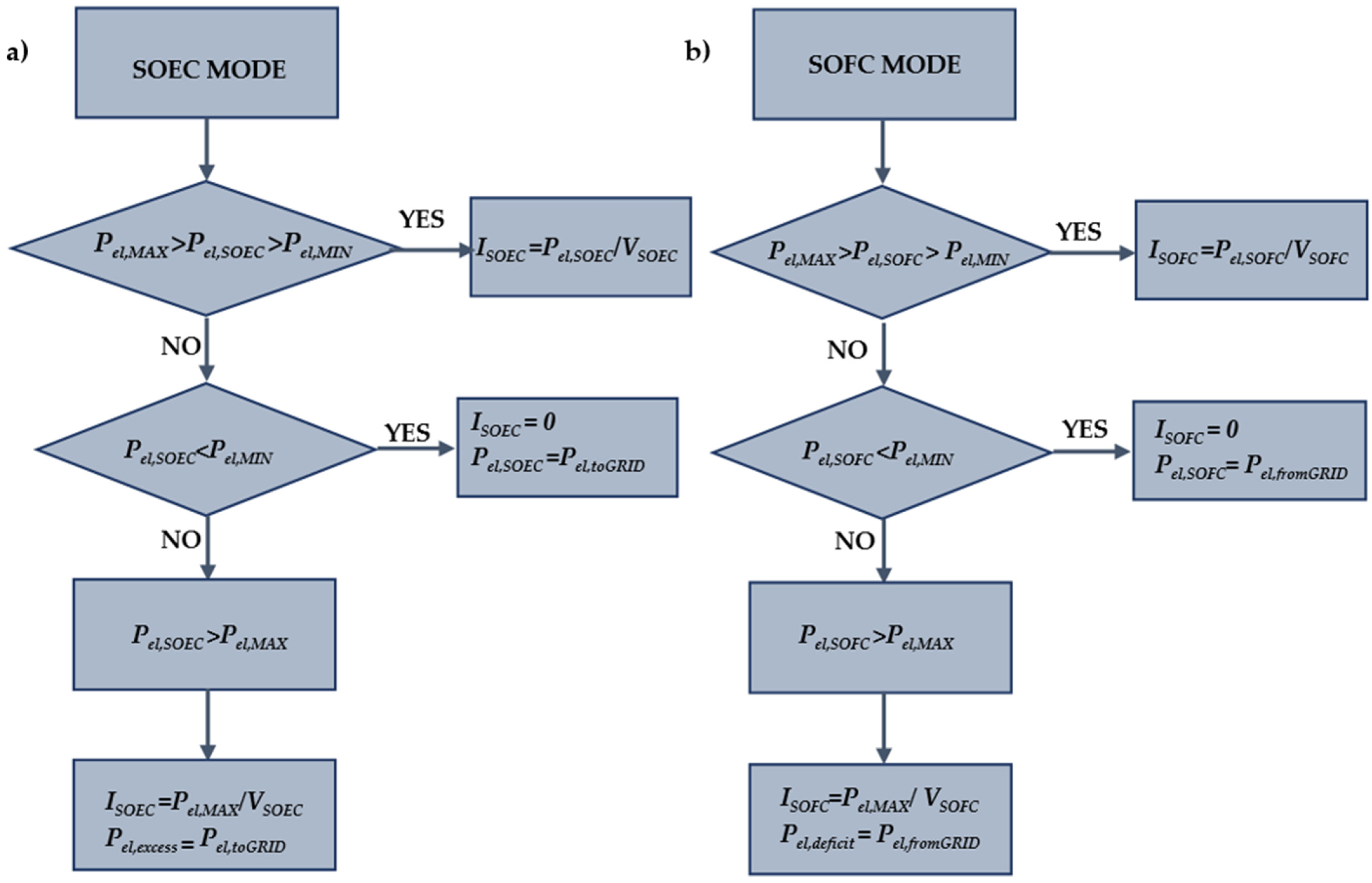
- The dynamic analysis of a hybrid renewable system for hydrogen production and storage is carried out by means of a reversible SOC model validated in MATLAB®;
- Several control strategies are implemented and discussed both for the operation of the fuel cell and hydrogen storage; furthermore, temperature operating conditions of the cell are managed;
- A well-developed thermoeconomic analysis is proposed to evaluate the energy and environmental savings along with the economic feasibility;
- A thermoeconomic analysis focused on the hydrogen storage is made to select the optimal size of the H2 storage for the proposed system;
- The analysis of the power exchanged with the grid is carried out to investigate how the local grid overloading conditions are avoided by means of the proposed technology.
2. Solid-Oxide Cell Model
3. System Model
3.1. TRNSYS Model
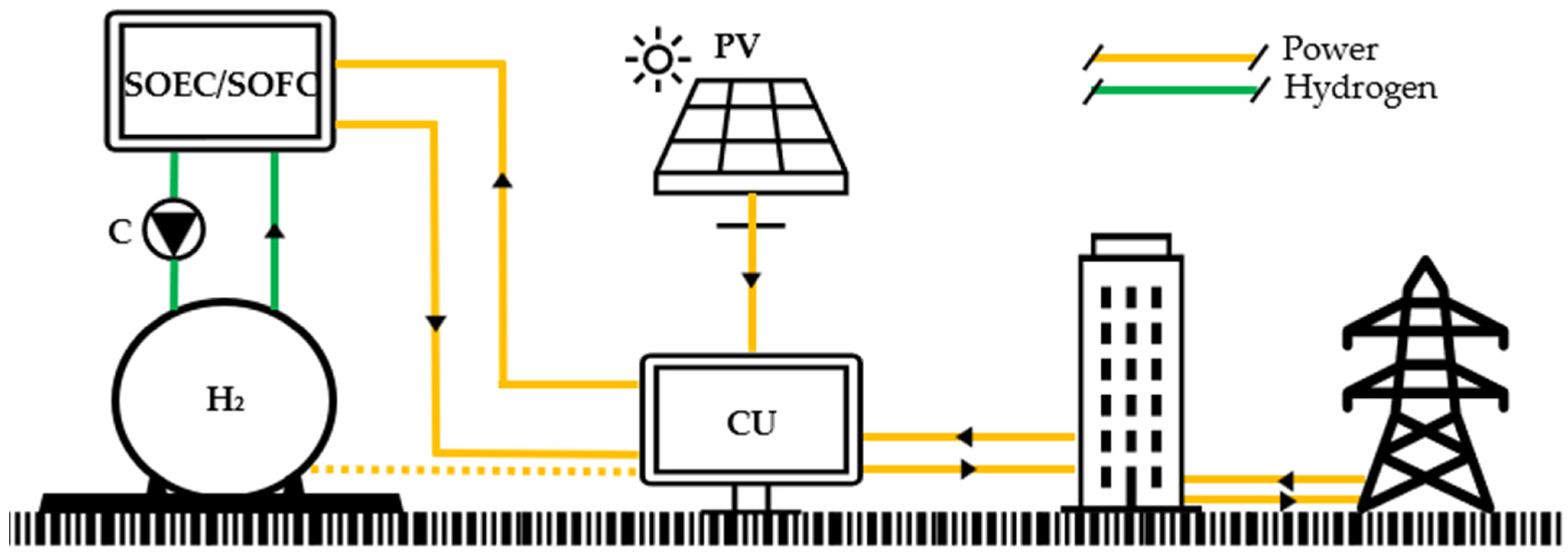
- The PV field component is modeled by means of type94, which considers an equivalent electric circuit to determine the I–V curve of a PV module [34]. Solar radiation is given from another type, which uses data from METEONORM database [35]. This type is set in order to track the maximum power point (MPP). The electric power produced by the PV field is supplied to a DC/AC (direct current–alternate current) inverter to meet the electric load of the dwelling.
- The hydrogen storage is modeled by means of type164, which considers an ideal gas storage model. The volumetric flow rate of hydrogen entering and exiting the tank is evaluated in Nm3 (273.15 K and 1 bar); the same unit is used for the volume of gas stored. To simplify the model, the gas is supposed to be compressed inside the tank by neglecting the corresponding temperature increase cause.
- The hydrogen compressor is modeled by the authors by means of standard mechanical equations for the calculation of the compression work. The outlet temperature iswhere Tin is the inlet temperature; β is the compression ratio, in this case, the ratio between the tank pressure and the ambient pressure; and is the polytropic exponent, which is equal to 1.4 for the H2 since it is a diatomic gas [36].
3.2. Thermoeconomic Model
4. Case Study
5. Results and Discussion
5.1. SOC Model Validation
5.2. TRNSYS Model Validation
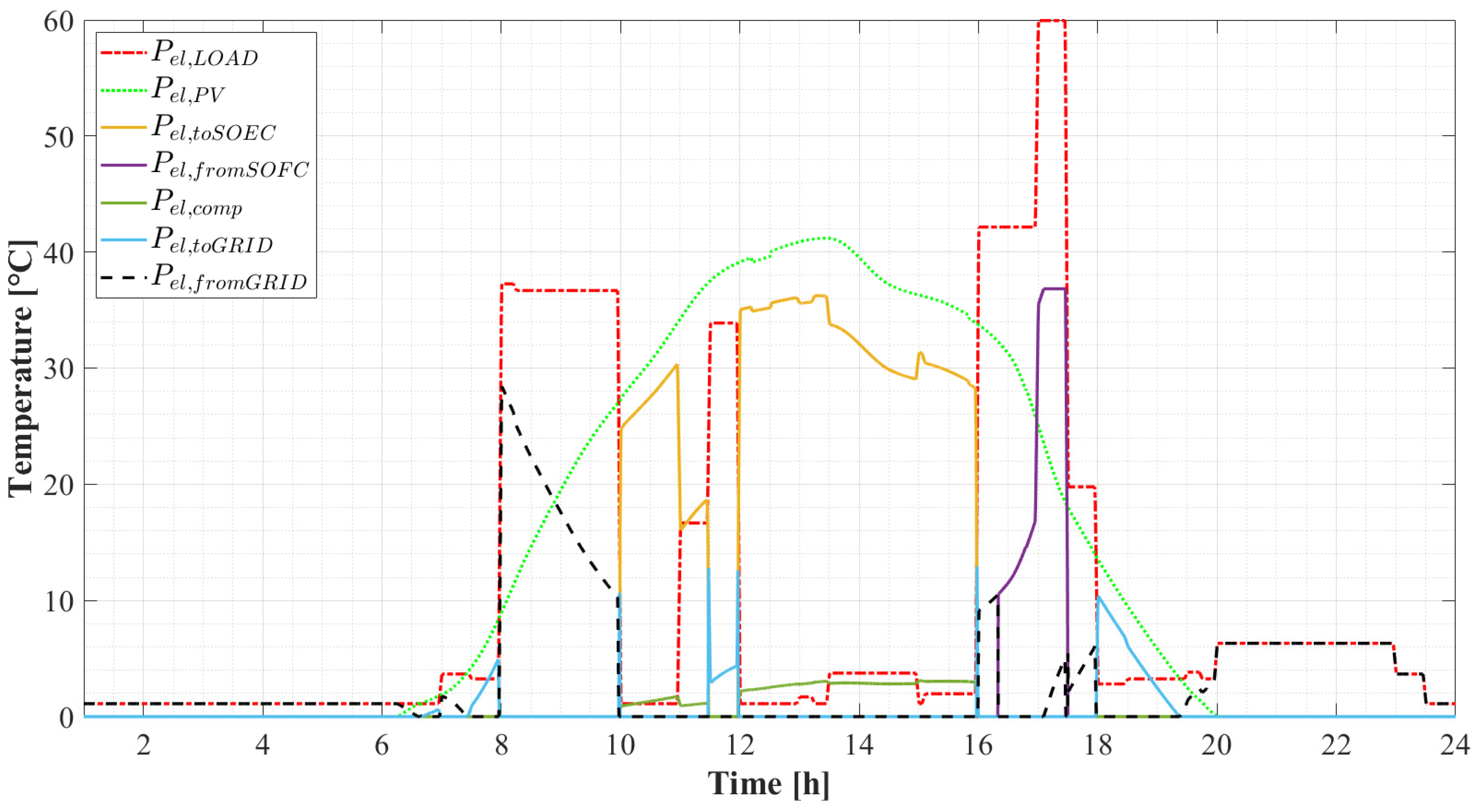
5.2.1. Daily Results
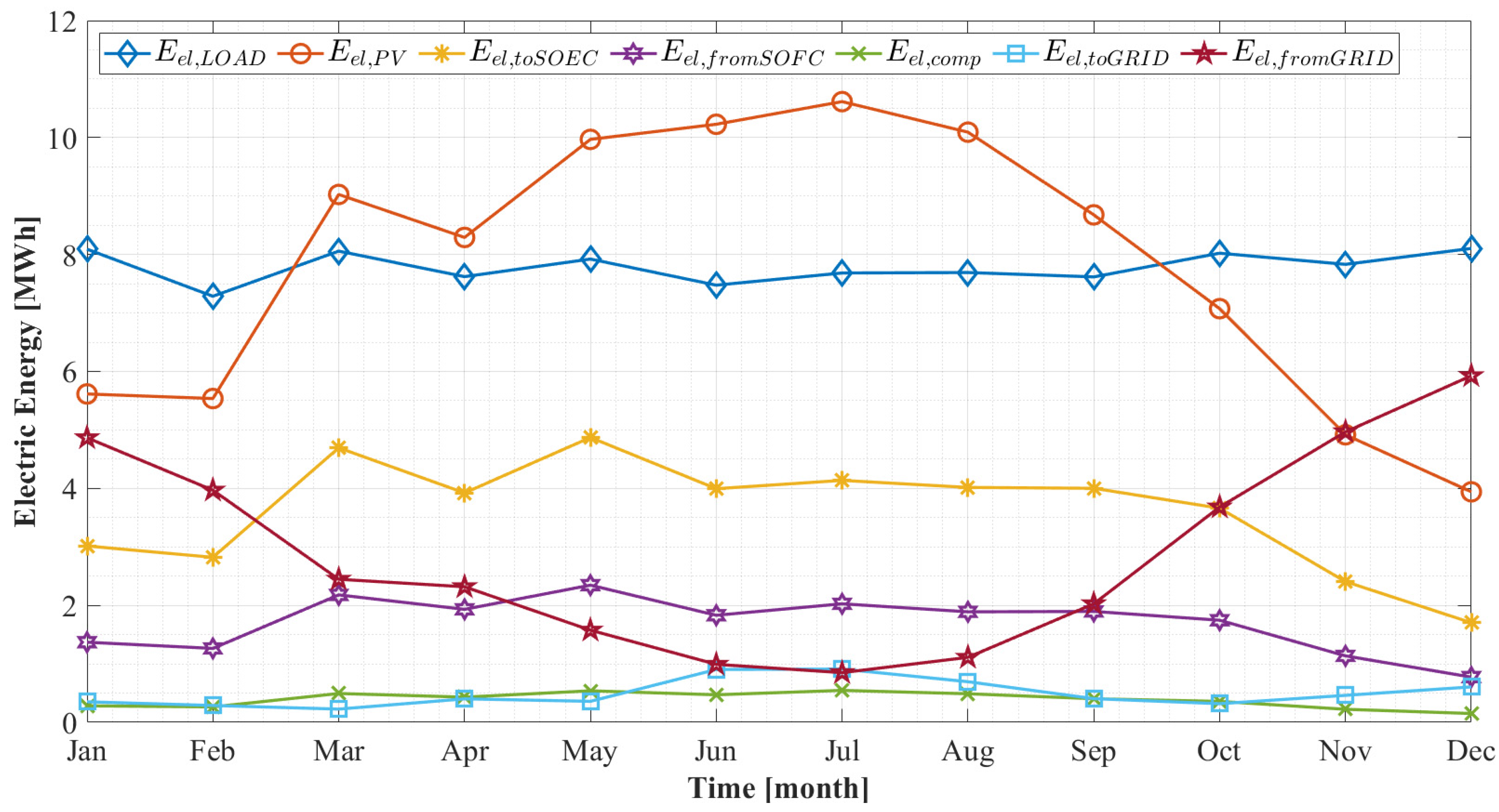
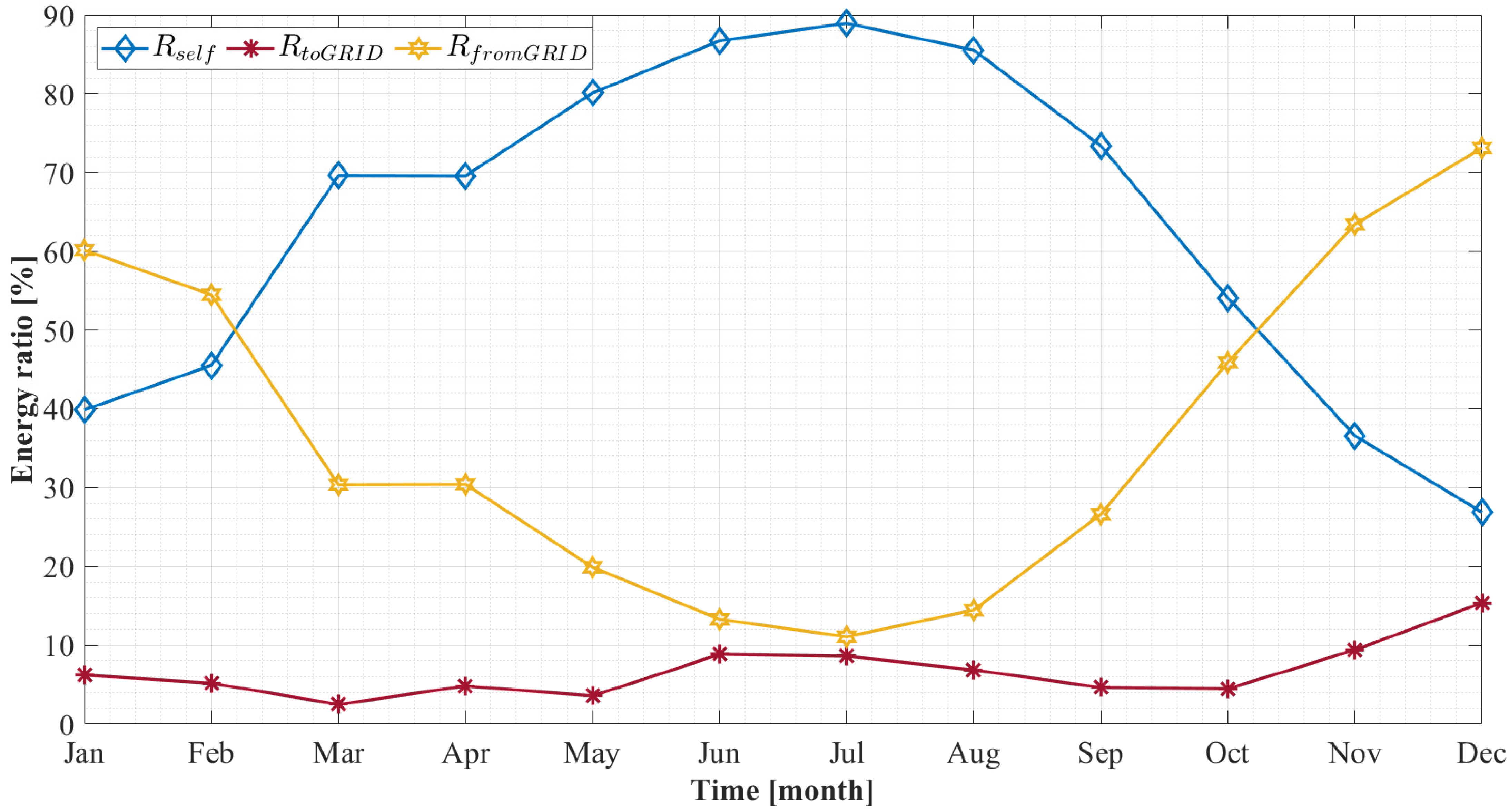
5.2.2. Monthly Results
5.2.3. Yearly Results
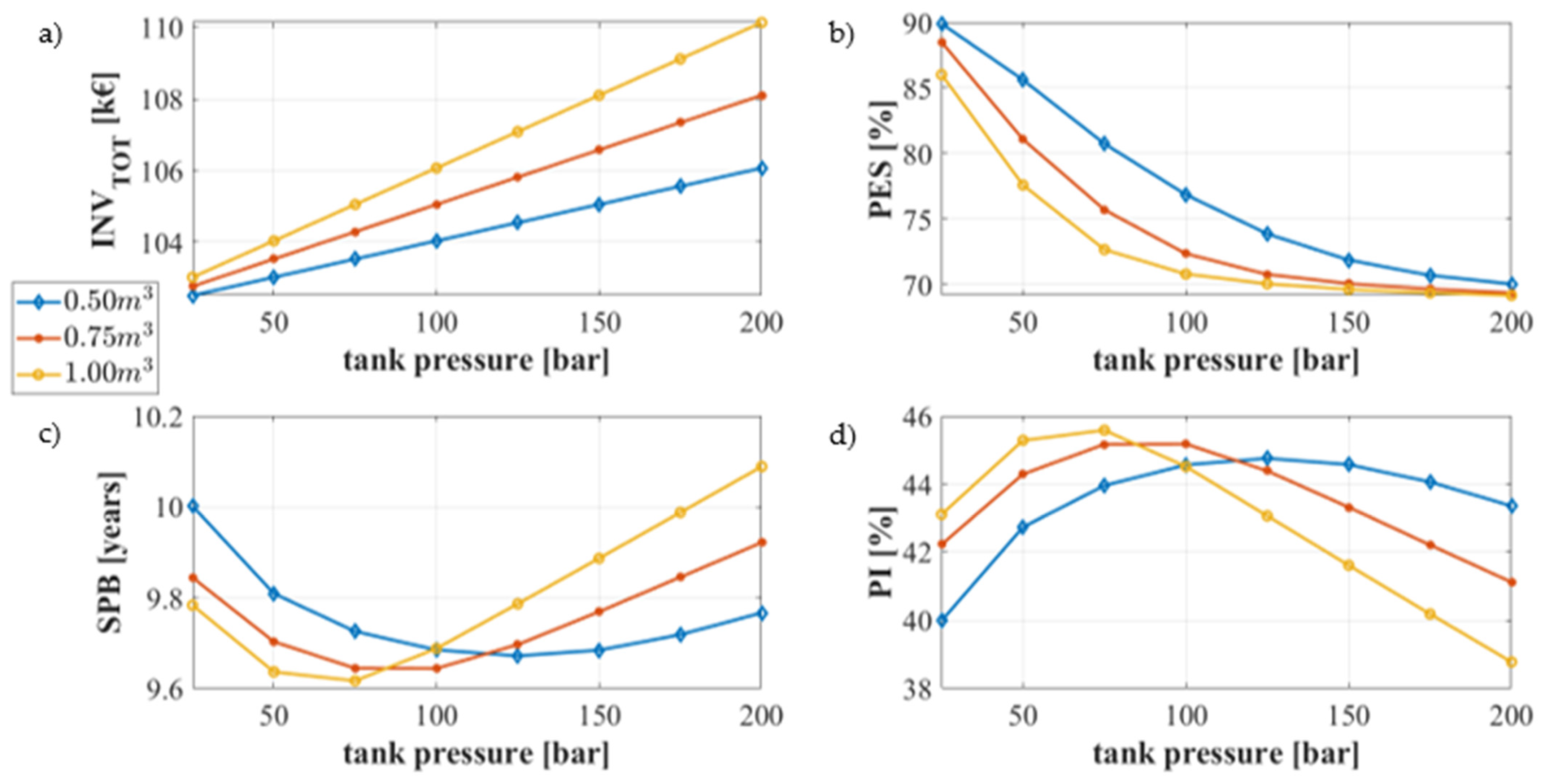
5.2.4. Parametric Analysis
6. Conclusions
- The overall efficiency of the system is very high compared to the other solid-oxide cell systems since the operating field is always in the optimal range of the cell. The global efficiency is, in fact, almost 47%;
- The storage system effectively reduces the peaks of the load since the interchanges with the grid are strongly reduced. In particular, the electricity sent to the grid is approximately 7% of the total PV production;
- The parametric analysis shows that the system leads to a primary energy saving of 73% within a simple pay-back period lower than 10 years. The system is also economically profitable, revealing a profit index of 46%.
Author Contributions
Funding
Institutional Review Board Statement
Informed Consent Statement
Data Availability Statement
Conflicts of Interest
Nomenclature
| GHG | Greenhouse gases |
| SOC | Solid oxide cell |
| HSS | Hydrogen storage system |
| P2H | Power to hydrogen |
| SMR | Steam methane reforming |
| RES | Renewable energy system |
| CSTR | Continuously stirred tank reactor |
| PEM | Proton exchange membrane |
| AEC | Alkaline electrolyzer cell |
| AFC | Alkaline fuel cell |
| DU | Degassing unit |
| COD | Chemical oxygen demand |
| NHES | Nuclear hybrid energy system |
| ASR | Area specific resistance (w/cm2) |
| PV | Photovoltaic |
| SOFC | Solid oxide fuel cell |
| CCS | Carbon capture and storage |
| SOEC | Solid oxide electrolyzer cell |
| OLR | Organic loading rate (kgCOD/(L d)) |
| PE | Primary energy (MWh) |
| SPB | Simple pay back (years) |
| NPV | Net present value (k€) |
| PI | Profit index (%) |
| PES | Primary energy saving (%) |
| LCOE | Levelized cost of energy (€) |
| n | Molar flow rate (mol/s) |
| i | Current density (mA/cm2) |
| p | Pressure (bar) |
| T | Temperature (°C) or (K) |
| V | Voltage (V) |
| F | Faraday’s constant (C/mol) |
| R | Gas constant (J/mol K) |
| P | Power (kW) |
| E | Energy (kWh) or (MWh) |
| Greek symbols | |
| α | Symmetry factor (adim.) |
| η | efficiency (adim.) |
References
- Masson-Delmotte, V.; Zhai, P.; Pirani, A.; Connors, S.L.; Péan, C.; Berger, S.; Caud, N.; Chen, Y.; Goldfarb, L.; Gomis, M.I.; et al. (Eds.) Climate Change 2021: The Physical Science Basis. Contribution of Working Group I to the Sixth Assessment Report of the Intergovernmental Panel on Climate Change; IPCC: Geneva, Switzerland; Cambridge University Press: Cambridge, UK, 2021. [Google Scholar]
- Bistline, J.; Blanford, G.; Mai, T.; Merrick, J. Modeling variable renewable energy and storage in the power sector. Energy Policy 2021, 156, 112424. [Google Scholar] [CrossRef]
- Hemmati, R.; Ghiasi, S.M.S.; Entezariharsini, A. Power fluctuation smoothing and loss reduction in grid integrated with thermal-wind-solar-storage units. Energy 2018, 152, 759–769. [Google Scholar] [CrossRef]
- Greiml, M.; Fritz, F.; Kienberger, T. Increasing installable photovoltaic power by implementing power-to-gas as electricity grid relief—A techno-economic assessment. Energy 2021, 235, 121307. [Google Scholar] [CrossRef]
- Abdin, Z.; Zafaranloo, A.; Radiee, A.; Merida, W.; Lipinski, W.; Khalilpour, L.R. Hydrogen as an energy vector. Renew. Sustain. Energy Rev. 2020, 120, 109620. [Google Scholar] [CrossRef]
- Zhang, C.; Wang, J.; Ren, Z.; Yu, Z.; Wang, P. Wind-powered 250 kW electrolyzer for dynamic hydrogen production: A pilot study. Int. J. Hydrogen Energy 2021, 46, 34550–34564. [Google Scholar] [CrossRef]
- Pein, M.; Neumann, N.C.; Venstrom, L.J.; Vieten, J.; Roeb, M.; Sattler, C. Two-step thermochemical electrolysis: An approach for green hydrogen production. Int. J. Hydrogen Energy 2021, 46, 24909–24918. [Google Scholar] [CrossRef]
- Parmar, K.R.; Pant, K.; Roy, S. Blue hydrogen and carbon nanotube production via direct catalytic decomposition of methane in fluidized bed reactor: Capture and extraction of carbon in the form of CNTs. Energy Convers. Manag. 2021, 232, 113893. [Google Scholar] [CrossRef]
- Ali Khan, M.H.; Daiyan, R.; Neal, P.; Haque, N.; MacGill, I.; Amal, R. A framework for assessing economics of blue hydrogen production from steam methane reforming using carbon capture storage & utilisation. Int. J. Hydrogen Energy 2021, 46, 22685–22706. [Google Scholar]
- Yu, M.; Wang, K.; Vredenburg, H. Insights into low-carbon hydrogen production methods: Green, blue and aqua hydrogen. Int. J. Hydrogen Energy 2021, 46, 21261–21273. [Google Scholar] [CrossRef]
- Rivera, X.C.S.; Topriska, E.; Kolokotroni, M.; Azapagic, A. Environmental sustainability of renewable hydrogen in comparison with conventional cooking fuels. J. Clean. Prod. 2018, 196, 863–879. [Google Scholar] [CrossRef]
- Thapa, B.S.; Neupane, B.; Yang, H.-S.; Lee, Y.-H. Green hydrogen potentials from surplus hydro energy in Nepal. Int. J. Hydrogen Energy 2021, 46, 22256–22267. [Google Scholar] [CrossRef]
- Rabiee, A.; Keane, A.; Soroudi, A. Technical barriers for harnessing the green hydrogen: A power system perspective. Renew. Energy 2020, 163, 1580–1587. [Google Scholar] [CrossRef]
- Ni, M.; Leung, M.K.; Leung, D.Y.; Sumathy, K. A review and recent developments in photocatalytic water-splitting using TiO2 for hydrogen production. Renew. Sustain. Energy Rev. 2007, 11, 401–425. [Google Scholar] [CrossRef]
- Schmidt, O.; Gambhir, A.; Staffell, I.; Hawkes, A.; Nelson, J.; Few, S. Future cost and performance of water electrolysis: An expert elicitation study. Int. J. Hydrogen Energy 2017, 42, 30470–30492. [Google Scholar] [CrossRef]
- Wang, S.; Li, W.; Fooladi, H. Performance evaluation of a polygeneration system based on fuel cell technology and solar photovoltaic and use of waste heat. Sustain. Cities Soc. 2021, 72, 103055. [Google Scholar] [CrossRef]
- Holmes-Gentle, I.; Tembhurne, S.; Suter, C.; Haussener, S. Dynamic system modeling of thermally-integrated concentrated PV-electrolysis. Int. J. Hydrogen Energy 2021, 46, 10666–10681. [Google Scholar] [CrossRef]
- Cao, Y.; Parikhani, T. A solar-driven lumped SOFC/SOEC system for electricity and hydrogen production: 3E analyses and a comparison of different multi-objective optimization algorithms. J. Clean. Prod. 2020, 271, 122457. [Google Scholar] [CrossRef]
- Martín-García, Í.; Rosales-Asensio, E.; González-Martínez, A.; Bracco, S.; Delfino, F.; de Simón-Martín, M. Hydrogen as an energy vector to optimize the energy exploitation of a self-consumption solar photovoltaic facility in a dwelling house. Energy Rep. 2020, 6, 155–166. [Google Scholar] [CrossRef]
- Al-Khori, K.; Bicer, Y.; Koç, M. Comparative techno-economic assessment of integrated PV-SOFC and PV-Battery hybrid system for natural gas processing plants. Energy 2021, 222, 119923923. [Google Scholar] [CrossRef]
- Elberry, A.M.; Thakur, J.; Santasalo-Aarnio, A.; Larmi, M. Large-scale compressed hydrogen storage as part of renewable electricity storage systems. Int. J. Hydrogen Energy 2021, 46, 15671–15690. [Google Scholar] [CrossRef]
- Okundamiya, M. Size optimization of a hybrid photovoltaic/fuel cell grid connected power system including hydrogen storage. Int. J. Hydrogen Energy 2020, 46, 30539–30546. [Google Scholar] [CrossRef]
- Wang, Q.; Liu, C.; Luo, R.; Li, X.; Li, D.; Macián-Juan, R. Thermo-economic analysis and optimization of the very high temperature gas-cooled reactor-based nuclear hydrogen production system using copper-chlorine cycle. Int. J. Hydrogen Energy 2021, 46, 31563–31585. [Google Scholar] [CrossRef]
- Ho, A.; Mohammadi, K.; Memmott, M.; Hedengren, J.; Powell, K.M. Dynamic simulation of a novel nuclear hybrid energy system with large-scale hydrogen storage in an underground salt cavern. Int. J. Hydrogen Energy 2021, 46, 31143–31157. [Google Scholar] [CrossRef]
- Caglayan, D.G.; Weber, N.; Heinrichs, H.U.; Linßen, J.; Robinius, M.; Kukla, P.A.; Stolten, D. Technical potential of salt caverns for hydrogen storage in Europe. Int. J. Hydrogen Energy 2020, 45, 6793–6805. [Google Scholar] [CrossRef]
- Karacavus, B.; Aydın, K. Hydrogen production and storage analysis of a system by using TRNSYS. Int. J. Hydrogen Energy 2020, 45, 34608–34619. [Google Scholar] [CrossRef]
- Wang, C.; Chen, M.; Liu, M.; Yan, J. Dynamic modeling and parameter analysis study on reversible solid oxide cells during mode switching transient processes. Appl. Energy 2020, 263, 114601. [Google Scholar] [CrossRef]
- Hajimolana, S.A.; Hussain, M.A.; Daud, W.A.W.; Soroush, M.; Shamiri, A. Mathematical modeling of solid oxide fuel cells: A review. Renew. Sustain. Energy Rev. 2011, 15, 1893–1917. [Google Scholar] [CrossRef]
- Zeng, Z.; Qian, Y.; Zhang, Y.; Hao, C.; Dan, D.; Zhuge, W. A review of heat transfer and thermal management methods for temperature gradient reduction in solid oxide fuel cell (SOFC) stacks. Appl. Energy 2020, 280, 115899. [Google Scholar] [CrossRef]
- Somano, V.; Ferrero, D.; Santarelli, M.; Papurello, D. CFD model for tubular SOFC directly fed by biomass. Int. J. Hydrogen Energy 2021, 46, 17421–17434. [Google Scholar] [CrossRef]
- Pianko-Oprych, P.; Jaworski, Z.; Kendall, K. Cell, Stack and System Modelling. In High-Temperature Solid Oxide Fuel Cells for the 21st Century, 2nd ed.; Kendall, K., Kendall, M., Eds.; Academic Press: Cambridge, MA, USA, 2016; Chapter 13; pp. 407–460. [Google Scholar]
- Sundén, B. Modeling approaches for fuel cells. In Hydrogen, Batteries and Fuel Cells; Sundén, B., Ed.; Academic Press: Cambridge, MA, USA, 2019; Chapter 10; pp. 167–202. [Google Scholar]
- Kalogirou, S.A. Designing and Modeling Solar Energy Systems. In Solar Energy Engineering, 2nd ed.; Kalogirou, S.A., Ed.; Academic Press: Cambridge, MA, USA, 2014; Chapter 11; pp. 583–699. [Google Scholar]
- Calise, F.; Cappiello, F.L.; Dentice d’Accadia, M.; Vicidomini, M. Dynamic modelling and thermoeconomic analysis of micro wind turbines and building integrated photovoltaic panels. Renew. Energy 2020, 160, 633–652. [Google Scholar] [CrossRef]
- Bellemare, C.; Labelle, D. Hourly meteorological data files adapted for main frame computer programs and for microcomputer programs. In Intersol Eighty Five; Bilgen, E., Hollands, K.G.T., Eds.; Pergamon: Oxford, UK, 1986; pp. 2420–2423. [Google Scholar]
- Moran, M.J. Fundamentals of Engineering Thermodynamics, 6th ed.; Wiley: Hoboken, NJ, USA, 2008. [Google Scholar]
- Calise, F.; Cappiello, F.L.; Dentice, M.; Vicidomoni, M. Concentrating photovoltaic/thermal collectors coupled with an anaerobic digestion process: Dynamic simulation and energy and economic analysis. J. Clean. Prod. 2021, 311, 127363. [Google Scholar] [CrossRef]
- Singh, S.P.; Ohara, B.; Ku, A.Y. Prospects for cost-competitive integrated gasification fuel cell systems. Appl. Energy 2021, 290, 116753. [Google Scholar] [CrossRef]
- Carr, S.; Premier, G.C.; Guwy, A.J.; Dinsdale, R.M.; Maddy, J. Hydrogen storage and demand to increase wind power onto electricity distribution networks. Int. J. Hydrogen Energy 2014, 39, 10195–10207. [Google Scholar] [CrossRef]
- Calise, F.; Cappiello, F.L.; D’Accadia, M.D.; Vicidomini, M. Energy efficiency in small districts: Dynamic simulation and technoeconomic analysis. Energy Convers. Manag. 2020, 220, 113022. [Google Scholar] [CrossRef]


| Parameter | Description | Value | Unit |
|---|---|---|---|
| jel,fromGRID | Unit cost of the electric energy | 0.18 | €/kWh |
| jel,toGRID | Unit sell price of the electric energy | 0.06 | €/kWh |
| fEE | CO2 equivalent emission factor for the electric energy | 0.483 | kgCO2/kWh |
| LHVH2 | Hydrogen lower heating value | 11.109 | MJ/Nm3 |
| CPV | PV unit cost | 1000 | €/kW |
| CSOC | SOC unit cost | 1000 | €/kW |
| Cstorage | Hydrogen tank unit cost | 5000 | €/kg |
| Component | Parameter | Description | Value | Unit |
|---|---|---|---|---|
| PV PANEL | Amodule,PV | PV module area | 1.609 | m2 |
| Pel,PV | PV field rated power | 50 | kW | |
| Nseries | Number of modules in series | 2 | - | |
| Nparalel | Number of modules in parallel | 100 | ||
| Isc,ref | Module short-circuit current at reference conditions | 8.94 | A | |
| voc,ref | Module open-circuit voltage at reference conditions | 37.3 | V | |
| Tc,ref | Reference temperature | 298 | K | |
| Gtot,ref | Reference insolation | 1000 | W/m2 | |
| vmp,ref | Module voltage at max power point and reference conditions | 30.1 | V | |
| Imp,ref | Module current at max power point and reference conditions | 8.64 | A | |
| μIsc | Temperature coefficient of Isc at (ref. condition) | 0.0004 | 1/K | |
| μvoc | Temperature coefficient of voc (ref. condition) | −0.003 | ||
| Tc,NOCT | Module temperature at NOCT | 319 | K | |
| Tc,ref | Ambient temperature at NOCT | 293 | ||
| Electrolizer-Fuel Cell | Prcell | Cell operative pressure | 1 | bar |
| Acell | Cell area | 87.7 | cm2 | |
| ncell | Number of cells in series | 8 | - | |
| nstack | Number of stacks in parallel | 50 | ||
| Pel,EC,min | Minimum power allowed to SOEC | 13.15 | kW | |
| Pel,EC,max | Maximum power allowed to SOEC | 48.23 | kW | |
| Pel,FC,min | Minimum power allowed from SOFC | 10.52 | kW | |
| Pel,FC,max | Maximum power allowed from SOFC | 36.83 | kW | |
| Pel,FC/Pel,EC | Rated fuel cell/electrolyzer capacity | 45/50 | kW | |
| H2 storage | V | Tank volume | 1 | m3 |
| PrTK,max | Maximum tank pressure | 200 | bar | |
| Compressor | ηIS | Compressor isentropic efficiency | 0.80 | - |
| Inverter | ηI | Inverter/Regulator efficiency | 0.96 | - |
| Feeding Gas | Flow Rate | Temperature | |
|---|---|---|---|
| - | [sccm/cm2] | [K] | |
| Anode | H2/H2O (50–50%) | 12.44 | 1033 |
| Chatode | O2 (100%) | 5.70 | 1033 |
| Parameter | Value | Unit |
|---|---|---|
| Eel,toSOEC | 43.25 | MWh/year |
| Eel,fromSOFC | 20.39 | MWh/year |
| Eel,comp | 4.65 | MWh/year |
| Eel,toGRID | 5.92 | MWh/year |
| Eel,fromGRID | 34.73 | MWh/year |
| Eel,toTANK | 45.23 | MWh/year |
| Eel,fromTANK | 44.43 | MWh/year |
| Eel,self | 58.67 | MWh/year |
| RS | PS | ||
|---|---|---|---|
| PE | [MWh/year] | 203.05 | 75.50 |
| PES | [%] | - | 69 |
| CO2 | [tCO2/year] | 44.83 | 16.67 |
| ΔCO2 | [%] | - | 69 |
| C | [k€/year] | 16.81 | 5.90 |
| ΔC | [k€/year] | - | 10.92 |
| ΔC | [%] | - | 65 |
| INV | [k€] | - | 110.13 |
| SPB | [years] | - | 10.1 |
| NPV | [k€] | - | 42.70 |
| PI | [%] | - | 39 |
Publisher’s Note: MDPI stays neutral with regard to jurisdictional claims in published maps and institutional affiliations. |
© 2021 by the authors. Licensee MDPI, Basel, Switzerland. This article is an open access article distributed under the terms and conditions of the Creative Commons Attribution (CC BY) license (https://creativecommons.org/licenses/by/4.0/).
Share and Cite
Calise, F.; Cappiello, F.L.; Cimmino, L.; Dentice d’Accadia, M.; Vicidomini, M. Dynamic Simulation and Thermoeconomic Analysis of a Hybrid Renewable System Based on PV and Fuel Cell Coupled with Hydrogen Storage. Energies 2021, 14, 7657. https://doi.org/10.3390/en14227657
Calise F, Cappiello FL, Cimmino L, Dentice d’Accadia M, Vicidomini M. Dynamic Simulation and Thermoeconomic Analysis of a Hybrid Renewable System Based on PV and Fuel Cell Coupled with Hydrogen Storage. Energies. 2021; 14(22):7657. https://doi.org/10.3390/en14227657
Chicago/Turabian StyleCalise, Francesco, Francesco Liberato Cappiello, Luca Cimmino, Massimo Dentice d’Accadia, and Maria Vicidomini. 2021. "Dynamic Simulation and Thermoeconomic Analysis of a Hybrid Renewable System Based on PV and Fuel Cell Coupled with Hydrogen Storage" Energies 14, no. 22: 7657. https://doi.org/10.3390/en14227657
APA StyleCalise, F., Cappiello, F. L., Cimmino, L., Dentice d’Accadia, M., & Vicidomini, M. (2021). Dynamic Simulation and Thermoeconomic Analysis of a Hybrid Renewable System Based on PV and Fuel Cell Coupled with Hydrogen Storage. Energies, 14(22), 7657. https://doi.org/10.3390/en14227657