Intelligent Algorithm for Variable Scale Adaptive Feature Separation of Mechanical Composite Fault Signals

Abstract

With the development of modern industry and scientific technology, production equipment plays an increasingly important role in military and industrial production, and the fault detection signal of gears and bearings state in transmission equipment becomes very important. Therefore, this paper proposes a gear-bearing composite fault signal decomposition and reconstruction method, which combines the marine predator algorithm (MPA) and variational mode decomposition (VMD) technologies. For the parameters’ selection of VMD, the optimization algorithm allows us to quickly and accurately obtain the results with the best kurtosis correlation index after signal decomposition and reconstruction. The experiments demonstrate the excellent performance of our method in the field of separation and denoising mixed gear-bearing fault signals.

1. Introduction

Equipment condition monitoring and fault diagnosis technologies have become an urgent need for equipment management and maintenance. These technologies can foresee accidents, ensure personal equipment safety, and also greatly improve production efficiency. At present, one of the common fault diagnosis methods is the analysis of the vibration signals of individual drive components [1]. However, compound faults of gears and bearings occur extremely frequently in common transmission component problems [2]. Therefore, the research on the separation of the characteristics of gear and bearing compound faults is of great significance.

Efficient planning of the energy that exists in all aspects of society, such as consumption [3] and fuel [4,5,6,7], is an important study. Zhang et al. [6] proposed a model combining genetic algorithms and neural networks to improve the accuracy of wind energy prediction and, thus, effectively enhance the development and utilization of energy. This paper focuses on the effective decomposition and reconstruction of the fault signal energy of transmission devices in mechanical engineering. Signal decomposition plays an important role in fault diagnosis [8,9]. Soualhi A [9] uses empirical mode decomposition (EMD), together with the Hilbert transform (HT), to extract the temporal components of the vibration signal, and then performs classification to monitor the signal. Variable mode decomposition (VMD) plays an important role in the separation of mechanical compound fault signals [10]. It is mainly a variational problem based on Wiener Hilbert transformations and frequency mixing. VMD determines the central frequencies and bandwidths of several band-limited intrinsic mode functions [11]. VMD adaptively separates the frequency domain and modal components of the signal, under the condition that the sum of the estimated bandwidths of each component is minimized. Huang et al. [12] proposed a method to denoise the original signal by combining VMD and simultaneous wavelet transform (SSWT) algorithms. Zhong et al. [13] proposed a new method to distinguish foreign object debris (FOD) signals from clutter signals, based on optimal VMD and support vector data description (SVDD). Usually, experimenters follow the experimental experience to give the parameters of VMD. However, the improper choice of parameters may eliminate part of the off-scale noise and even some useful target information by mistake. There have been some studies on parameter optimization for VMD [14,15,16]. For example, Zhang et al. [14] used the bacterial foraging algorithm (BFA) to obtain the best combination of VMD parameters.

In this paper, we use the marine predator algorithm (MPA) to find the optimal modal number and penalty factor in VMD. The composite signal is decomposed according to the optimal parameters. Then, the bearing and gear signals are reconstructed separately with more effective information, based on the proposed new fault characteristic frequency index (FCFI) index. Experimental results also demonstrate that the signal obtained by our method has a better index, which means a better separation of the bearing and gear signals. The contributions of this paper are summarized in the following two points:

1. We proposed a variable-scale, adaptive feature separation method, based on VMD and MPA algorithms, applied it to the feature separation of gear-bearing composite fault signals, and realized the fault signal reconstruction.

2. In the signal separation and reconstruction, the intelligent algorithm MPA was introduced. The algorithm aimed to minimize the kurtosis of the reconstructed signal and realized the iterative solution of VMD parameters.

This paper contains the following sections. Section 1 introduces the research background and motivation of this paper. Section 2 gives the simulation signals and related parameters required for the experiments, which lays the foundation for the experiments to be conducted later. Section 3 introduces our variable-scale adaptive feature separation method, which specifically includes the method framework, decomposition and reconstruction of composite signals, and optimizations of VMD parameters based on MPA. Section 4 shows the experimental results and analysis. Section 5 summarizes the work of this paper.

2. Sensing Systems and Signal Models

For gears and rolling bearings, due to the uniqueness of the measured object, the vibration signal is mainly concentrated in the middle and high frequency parts, so we generally choose vibration acceleration sensors to measure the faults [17]. This paper is an analysis of the composite fault signal of gear-bearing in a gearbox. Based on the gear and bearing fault characteristics in the actual transmission system, we define the expression of the fault vibration signal in the time domain as follows [1].

$$\begin{array}{cc}\hfill & f\left(t\right)=x_g\left(t\right)+x_b\left(t\right)+n\left(t\right)\hfill \\ \hfill & x_g\left(t\right)=\sum _{p=1}^P{A}_{p}cos\left(2\pi p{f}_{p}t\right)[1+\sum _{q=1}^Q{B}_q^{p}cos\left(2\pi q{f}_{r}t\right)]\hfill \\ \hfill & x_b\left(t\right)=e^{-bT}\sum _{i=1}^I{C}_{i}sin\left(2\pi n{f}_{ci}t\right)T=mod(t,1/f_o).\hfill \end{array}$$

(1)

The fault signal ($x\left(t\right)$) consists of the vibration signals induced by the local faults in gears ($x_g\left(t\right)$) and bearings ($x_b\left(t\right)$), as well as the multi-scale strong noise signals ($n\left(t\right)$). Localized gear faults have a modulating effect on the meshing vibration of the gear. So, the gear vibration signal contains not only the meshing frequency and its harmonic components but also the side band structure, caused by amplitude and frequency modulation. In Equation (1), $f_p$ denotes the gear meshing frequency, $A_p$ is the harmonic amplitude of the carrier signal with the gear meshing frequency as the base wave, P and Q are the number of harmonics, $f_r$ denotes modulation frequency, and $B_q$ is the harmonic amplitude of the modulated signal with the gear rotation rate as the base wave. Common bearing faults modulate the vibration signal of the rotating bearing and create a fixed period of envelope variation in the fault signal. $x_b\left(t\right)$, $f_{ci}$, and $C_i$ are the resonant frequency and amplitude determined by the bearing structure, respectively. $f_o$ indicates the frequency of bearing failure, and b is the pulse attenuation coefficient. Other detailed simulation parameters can be found in Section 4.

3. Proposed Method

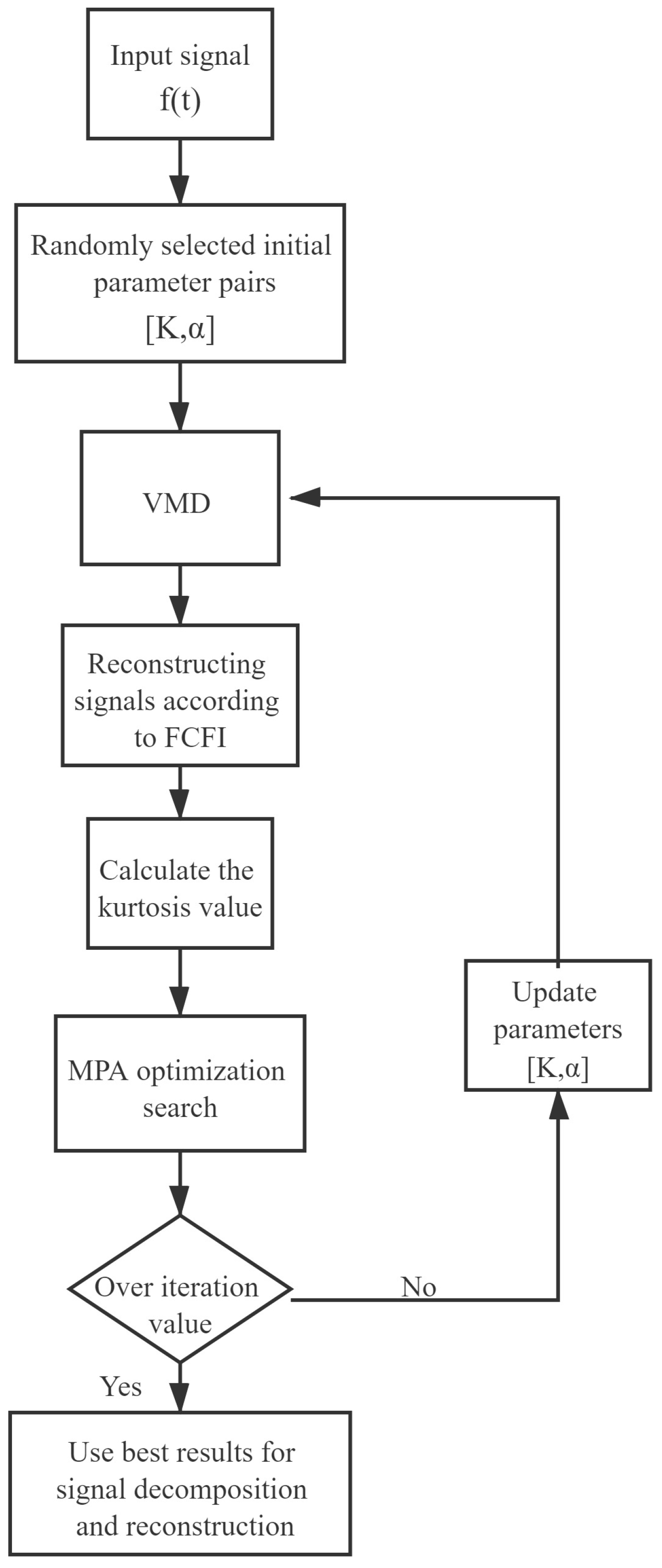
3.1. Algorithm Framework

The general framework of the multi-scale adaptive signal decomposition reconstruction method is shown in Figure 1. First, we randomly select 20 pairs of initial values [K,$\alpha$] and use them as parameters for VMD decomposition to generate 20 modules, each containing $k_i$ decomposition. Second, we classify each module based on FCFI metrics and reconstruct the gear and bearing failure signals. Then, we obtain the kurtosis value of the reconstructed signal by calculation. Third, we optimize the parameter selection by MPA algorithm with the objective of kurtosis minimization. Based on the currently solved parameter [K,$\alpha$], we iteratively loop the above steps to find the optimal parameter. Finally, we perform VMD decomposition, according to the optimal parameter results, and reconstruct the obtained components, according to FCFI. The following section details the VMD decomposition, module reconstruction, and MPA iterative optimization search methods.

3.2. VMD Decomposition and Reconfiguration

This section is divided into two parts, consisting of the decomposition and reconstruction of the composite signal.

3.2.1. Decomposition

First, the input signal ($f\left(t\right)$) is decomposed into K modal functions ($U_K\left(t\right)$). Then, a Hilbert variation is applied to each $U_K\left(t\right)$ to solve for the resolved signal and the predicted center frequency ($e^{-j{\omega }_{k}t}$). Next, we solve the variational problem to find $U_K\left(t\right)$, such that the sum of the estimated bandwidths of each mode is minimized, with the constraint that the sum of all $U_K\left(t\right)$ equals to the input signal $f\left(t\right)$.

$$\begin{array}{cc}\hfill & \underset{\left(U_k\right)\left({\omega }_k\right)}{min}\left\{\sum _k\left|\right|\partial t\left[\left(\delta \left(t\right)+\frac{j}{\pi t}\right)u_k\left(t\right)\right]e^{-j{\omega }_{k}t}{\left|\right|}_2^2\right\}\hfill \\ \hfill & s.t.\sum _{k=1}^K{u}_k=f\left(t\right)\hfill \end{array}$$

(2)

where $\partial t$ is the partial derivative of t, $\delta \left(t\right)$ is the shock function, and K is the number of modes obtained after decomposition.

With the Lagrange multiplier ($\gamma$) and quadratic penalty factor ($\alpha$), the transformation of Equation (2) leads to the Lagrange function of increasing type, as shown in Equation (3):

$$\begin{array}{cc}\hfill L(\left\{U_k\right\},\left\{{\omega }_k\right\},\gamma )& =\alpha \sum _k\left|\right|\partial t\left[\left(\delta \left(t\right)+\frac{j}{\pi t}\right)U_k\left(t\right)\right]e^{-j{\omega }_k\left(t\right)}{\left|\right|}_2^2\hfill \\ \hfill & +\left|\right|f\left(t\right)-\sum _k{U}_k\left(t\right){\left|\right|}_2^2+〈\gamma \left(t\right),f\left(t\right)-\sum _k{U}_k\left(t\right)〉.\hfill \end{array}$$

(3)

The modal components ($U_k$) and central frequency (${\omega }_k$), corresponding to the optimal solution of Equation (3), are given in Equation (4):

$$\begin{array}{cc}\hfill & {\widehat{U_k}}^{n+1}\left(\omega \right)=\frac{\widehat{f}\left(\omega \right)-{\displaystyle \sum _{i\ne k}}\widehat{U_i}\left(\omega \right)+\widehat{\lambda }\left(\omega \right)/2}{1+2\alpha {(\omega -{\omega }_k)}^2}\hfill \\ \hfill & {\omega }_k^{n+1}=\frac{{\int }_0^{\infty }\omega |\widehat{U_k}\left(\omega \right){|}^{2}d\omega }{{\int }_0^{\infty }|\widehat{U_k}\left(\omega \right){|}^{2}d\omega },\hfill \end{array}$$

(4)

where ${\widehat{U_k}}^{n+1}$ is the Wiener filter of the current residual, and $\widehat{f}(\omega )-{\displaystyle \sum _{i\ne k}}\widehat{U_i}\left(\omega \right)$, ${\omega }_k^{n+1}$ is the central frequency of the current modal function rate.

When the value of K is appropriate, the VMD can eliminate noise outside the frequency of each mode, thus highlighting the abrupt features of the signal and weakening the influence of the noise. When the value of $\alpha$ is appropriate, the VMD can guarantee the total signal bandwidth be the smallest possible, thus ensuring the accuracy of subsequent reconfigurations. Therefore, the selection of the correct and appropriate parameters is of great significance to the VMD decomposition results [18].

3.2.2. Reconfiguration

In order to obtain gear and bearing faults separately, this paper uses FCFI to identify the bearing fault information content in each model. The definition of FCFI is as follows:

$$FCFI=\sum _{i=1}^N(1/ran{k}_X(max\left(X\left(f\right){|}_{i\ast f_c-0.5bw⩽i\ast f_c+0.5bw}\right))),$$

(5)

where N denotes the order of the characteristic frequency of bearing failure, $ran{k}_X(•)$ denotes the index value in parentheses in the ranking after sorting the envelope spectrum amplitudes from largest to smallest, $max(•)$ denotes the maximum amplitude of the signal envelope spectrum $X\left(f\right)$ in the frequency range $i\ast f_c-0.5bw⩽i\ast f_c+0.5bw$, and $f_c$ denotes the bearing fault characteristic frequency.

3.3. MPA Algorithm

The modal number (K) and the penalty parameter ($\alpha$) have an important influence on the decomposition effect of VMD. However, there is no uniform or definite method for determining these two parameters. Intelligent optimization algorithms, such as the gray wolf [19] and genetic algorithms, were designed to achieve fast and efficient searches of global optimums. In order to achieve a better decomposition effect of VMD algorithm, this chapter uses the marine predator algorithm(MPA) to optimize the modal number (K) and penalty factor ($\alpha$) of VMD. MPA is one of the popular intelligent optimization algorithms, which is inspired by the survival of the fittest theory of the ocean. This algorithm has a stronger meritocracy and higher accuracy than other optimization algorithms [20].

Viswanathan [21] proposed that predators usually choose the optimal foraging strategy to maximize their contact rate with prey in their natural environment. In general, the next state or location of their foraging is dependent on the current state and transition probability to the next location. Similarly, in the ocean, many marine organisms follow the Levi’s flight pattern as the optimal foraging strategy [22]. It is a special type of stochastic swimming, characterized by many small steps, involving longer relocations, that come from probability distributions with power-law tails.

Similar to most heuristic optimization algorithms, MPA randomly initializes prey locations within the search space to initiate the optimization process. Each element ($x_{ij}$) of the prey matrix is initialized by:

$$x_{ij}=x_{min}+rand(x_{max}-x_{min}).$$

(6)

The final obtained prey matrix is of size $nd$, where n is the size of the population and d is the position of each dimension, i.e., the dimension of the solution to the problem. For each individual element in the prey matrix $x_i=\left[x_{i1},x_{i2},...,x_{id}\right]$, we calculate their fitness. Then n copies of the individual with the best result are used to form the Elite matrix.

Then we use three steps to complete the overall iterative process. First, when the number of iterations is less than one-third of the maximum number of iterations, we have

$$\begin{array}{cc}\hfill & s_i=R_B\otimes (Elit{e}_i-R_B\otimes Pre{y}_i),i=1...n\hfill \\ \hfill & Pre{y}_i=Pre{y}_i+P.R\otimes s_i,\hfill \end{array}$$

(7)

where $R_B$ is a vector, with dimension s, consisting of random numbers generated by using Brownian random walks, and d is the solution size of the problem; $s_i$ represents the step size of the move; P is a constant equal to 0.5; R is a vector consisting of uniformly distributed random numbers between 0 and 1 with dimension d; and $R_B$ obeys generalized Gaussian distribution. Each element ($R_{Bi}$) can be calculated by the following expression:

$${R_B}_i=\frac{1}{\sqrt{2\pi }}exp(-\frac{x^2}{2}).$$

(8)

Second, when the number of iterations is greater than one-third of the maximum number of iterations and less than two-thirds of it, we split the population into two parts for the operation. The first half of the population follows up the rules:

$$\begin{array}{cc}\hfill & s_i=R_L\otimes (Elit{e}_i-R_L\otimes Pre{y}_i),i=1...n/2\hfill \\ \hfill & Pre{y}_i=Pre{y}_i+P.R\otimes s_i,\hfill \end{array}$$

(9)

where $R_L$ is a vector coming out of the composition of the Levy distribution with dimension (d). Each element ($R_L$) can be calculated by the following expressions:

$$\begin{array}{cc}\hfill & R_{Li}=C\times \frac{x}{y^{1/a}},\hfill \\ \hfill & x=Normal(0,{{\sigma }_x}^2),{\sigma }_x={\left[\frac{\mathsf{\Gamma }(1+\beta )sin\left(\frac{\pi \beta }{2}\right)}{\mathsf{\Gamma }\left(\frac{1+\beta }{2}\right)\beta 2^{\frac{\beta -1}{2}}}\right]}^{1/\beta },\hfill \\ \hfill & y=Normal(0,{{\sigma }_y}^2),{\sigma }_y=1,\hfill \end{array}$$

(10)

where C and $\beta$ are constants equal to 0.05 and 1.5, respectively. The second half of the population update rule is as follows:

$$\begin{array}{cc}\hfill & s_i=R_B\otimes (R_B\otimes Elit{e}_i-Pre{y}_i),i=1...n/2\hfill \\ \hfill & Pre{y}_i=Elit{e}_i+P.CF\otimes s_i,\hfill \end{array}$$

(11)

where $CF$ is the adaptive parameter for the step size ($s_i$), which is defined as:

$$CF={(1-\frac{Iter}{Max\_Iter})}^{\left(2\frac{Iter}{Max\_Iter}\right)}.$$

(12)

Third, when the number of iterations is greater than two-thirds of the maximum number of iterations, the third stage is entered, and the population update rule are as follows:

$$\begin{array}{cc}\hfill & s_i=R_L\otimes (R_L\otimes Elit{e}_i-Pre{y}_i),i=1...n\hfill \\ \hfill & Pre{y}_i=Elit{e}_i+P.CF\otimes s_i.\hfill \end{array}$$

(13)

In the optimization process, we choose the inverse of the kurtosis as the judging criterion. We define that the main metric of the fault signal is the signal abrupt change degree. For mechanical transmission parts, kurtosis is one of the most commonly used indicators to characterize the degree of shock and sharpness of vibration signals, and it is a data statistic of the signal distribution characteristics [23]. For a discrete data set (x), its kurtosis is defined as:

$$Ku=\frac{E{(x-\mu )}^4}{{\sigma }^4},$$

(14)

where $E{(x-\mu )}^4$ is the fourth-order mathematical expectation, $\mu$ is the mean of x, and $\sigma$ is the standard deviation of x.

In our method, the specific steps of using MPA to find the optimal VMD decomposition parameters are as follows.

1. Set the algorithm parameters and initialize the population. To improve the computational efficiency and accuracy, the values of K and $\alpha$ are set to [1, 10] and [1000, 4000], respectively. Then we select 20 pairs of initial values from them as parameters for VMD decomposition, and then reconstruct the obtained components and calculate their signal kurtosis.

2. Calculate the fitness value, and record the optimal position.

3. According to the iterative phase, the predator updates its position by selecting the corresponding update method from Equations (7), (9), (11) and (13).

4. Calculate the fitness value, according to Equation (14), and update the optimal position.

5. Judge whether the stopping condition is satisfied, and if not, repeat steps 3–5; otherwise, output the optimal result of the algorithm.

4. Experiments and Results Analysis

In this section, we perform the experimental parameter setting, verify the convergence of the MPA algorithm, and analyze the results of the separation and reconstruction of the composite signal by the method in this paper. Finally, we quantitatively compare the performance of the tired different methods.

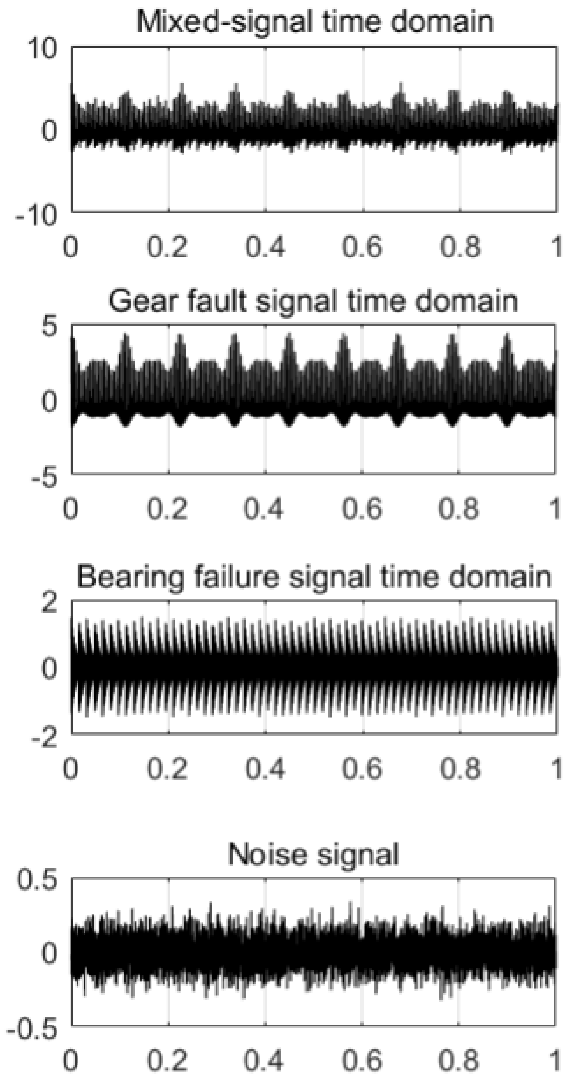
4.1. Experiment Settings

In this experiment, we simulated a signal with a duration of 1s and a sampling frequency of 6000 Hz, according to Equation (1), where the specific parameters were taken as shown in

Table 1. Compound fault signal simulation parameters.

Bearing Simulation Signal Parameters
Parameter Name	Numerical value
Resonant Frequency Order (I)	2
Resonant Frequency ($f_{ci}$)	[1600, 3000]
Gear Simulation Signal Parameters
Parameter Name	Numerical value
Engagement Frequency Order (P)	3
Magnitude Modulation Order (Q)	3
Engagement Frequency ($f_p$)	180
Engagement Frequency Amplitude ($A_p$)	[1, 1.2, 0.5]
Fault Frequency ($f_r$)	8.9
	[0.3, 0.15, 0.1]
Amplitude Modulation Factor ($B_q$)	[0.4, 0.25, 0.15]
	[0.2, 0.15, 0.05]
Outer Ring Fault Frequency ($f_o$)	62
Resonance Frequency Amplitude ($C_i$)	[1.5, 2]
Attenuation Coefficient (b)	100

. The time domain waveform of the simulated gear fault signal ($x_g\left(t\right)$), bearing fault signal ($x_b\left(t\right)$), multi-scale strong noise ($n\left(t\right)$), and mixed signal (main input signal) ($x\left(t\right)$) are, respectively, shown in Figure 2. From the Figure 2, it can be seen that the simulated gear and bearing fault signals have obvious modulation. However, it is difficult to find obvious modulation in the mixed signal after adding multi-scale strong noise.

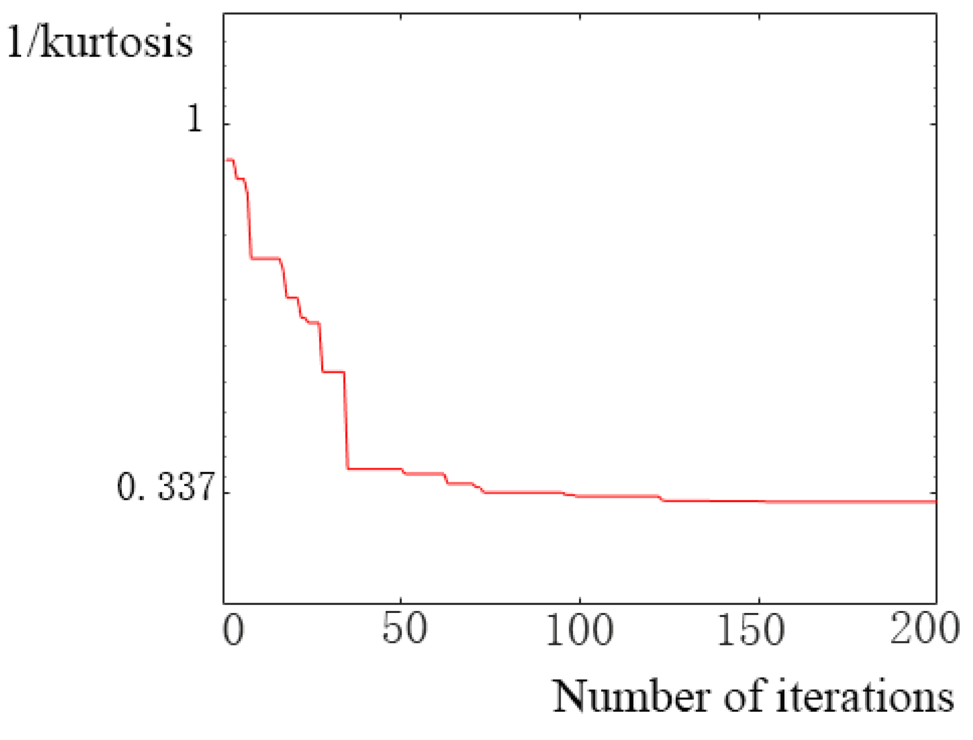
4.2. Parameter Optimization

VMD decomposition is performed on the main input signal ($f\left(t\right)$). The number of decomposition layers (K) ranges from [1, 10], and the traversal range of the penalty coefficient $\alpha$ is [1000, 4000]. The execution process of the MPA algorithm is shown in Figure 3. It can be seen from the figure that it gets the maximum kurtosis value of 2.97 that tends to converge. Meanwhile, it corresponds to K and $\alpha$ of 4 and 2200, respectively.

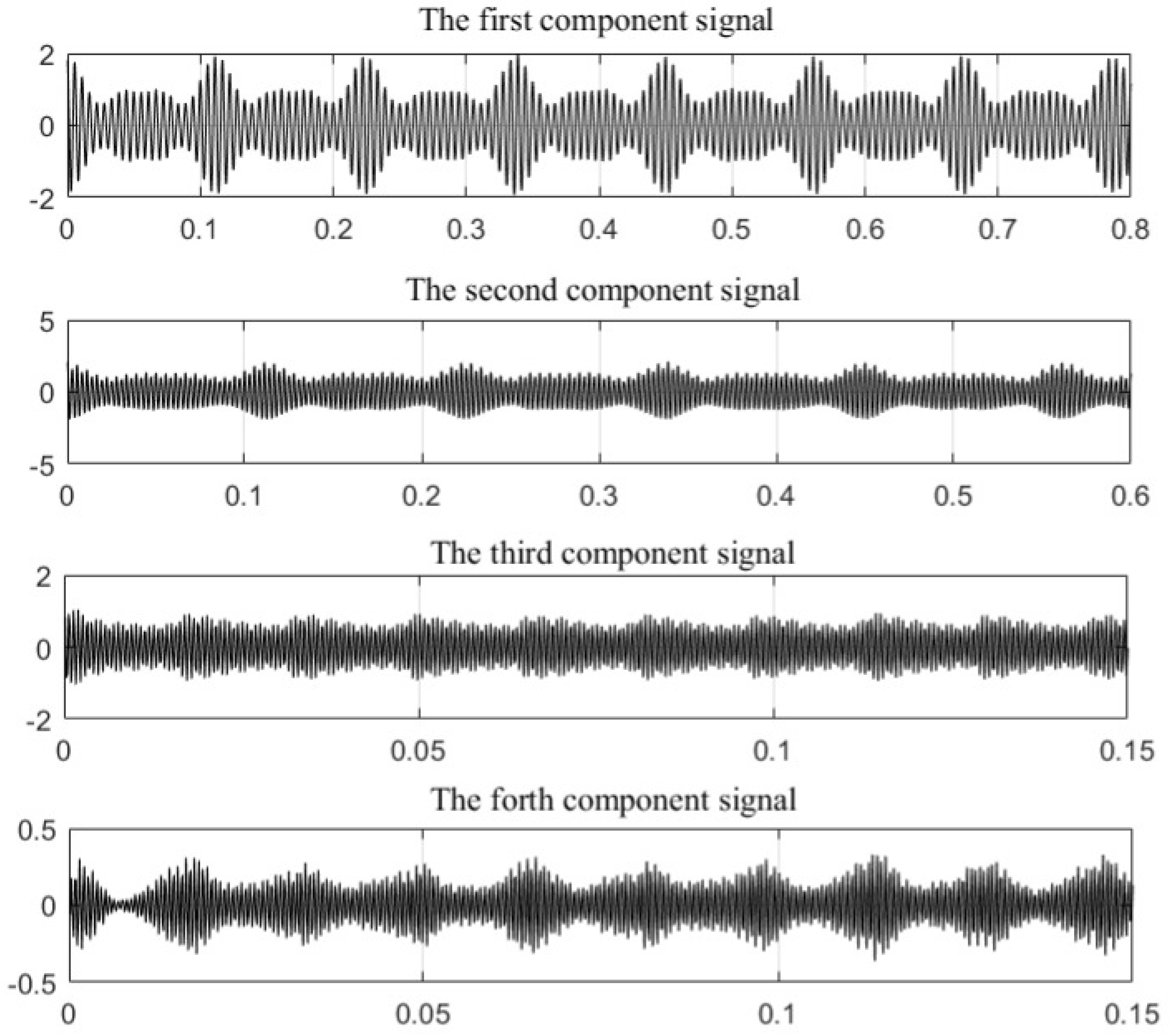
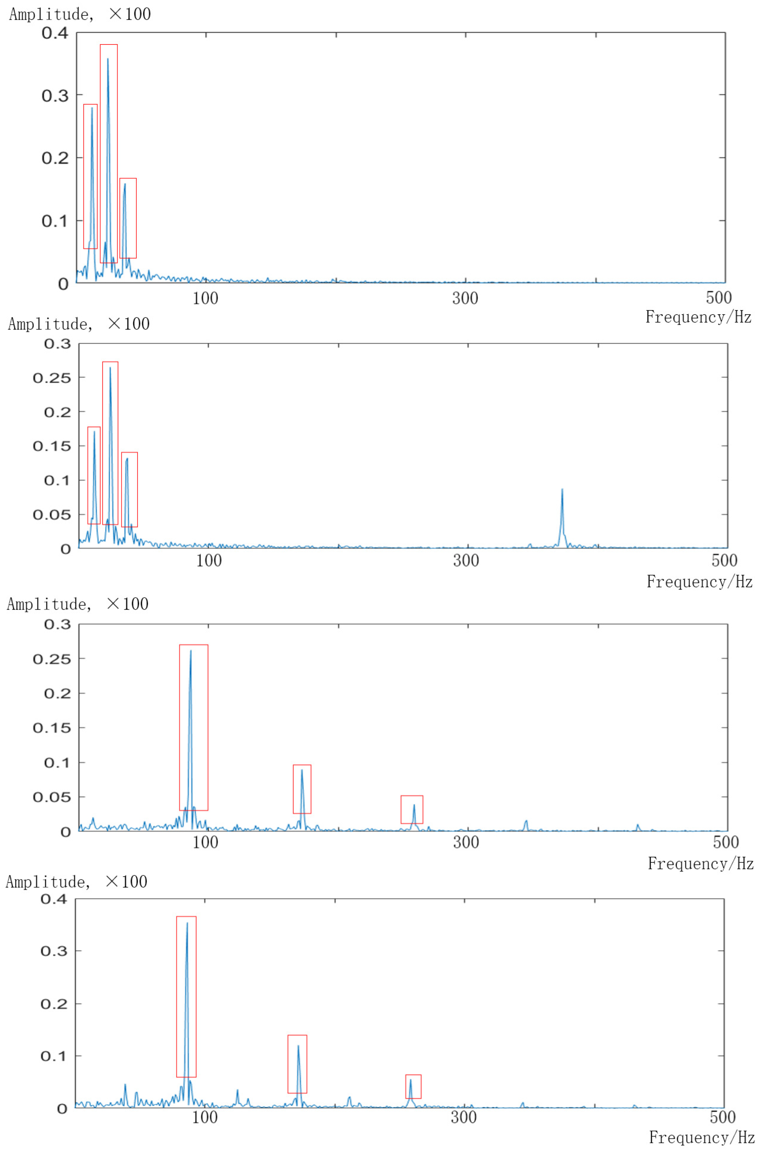
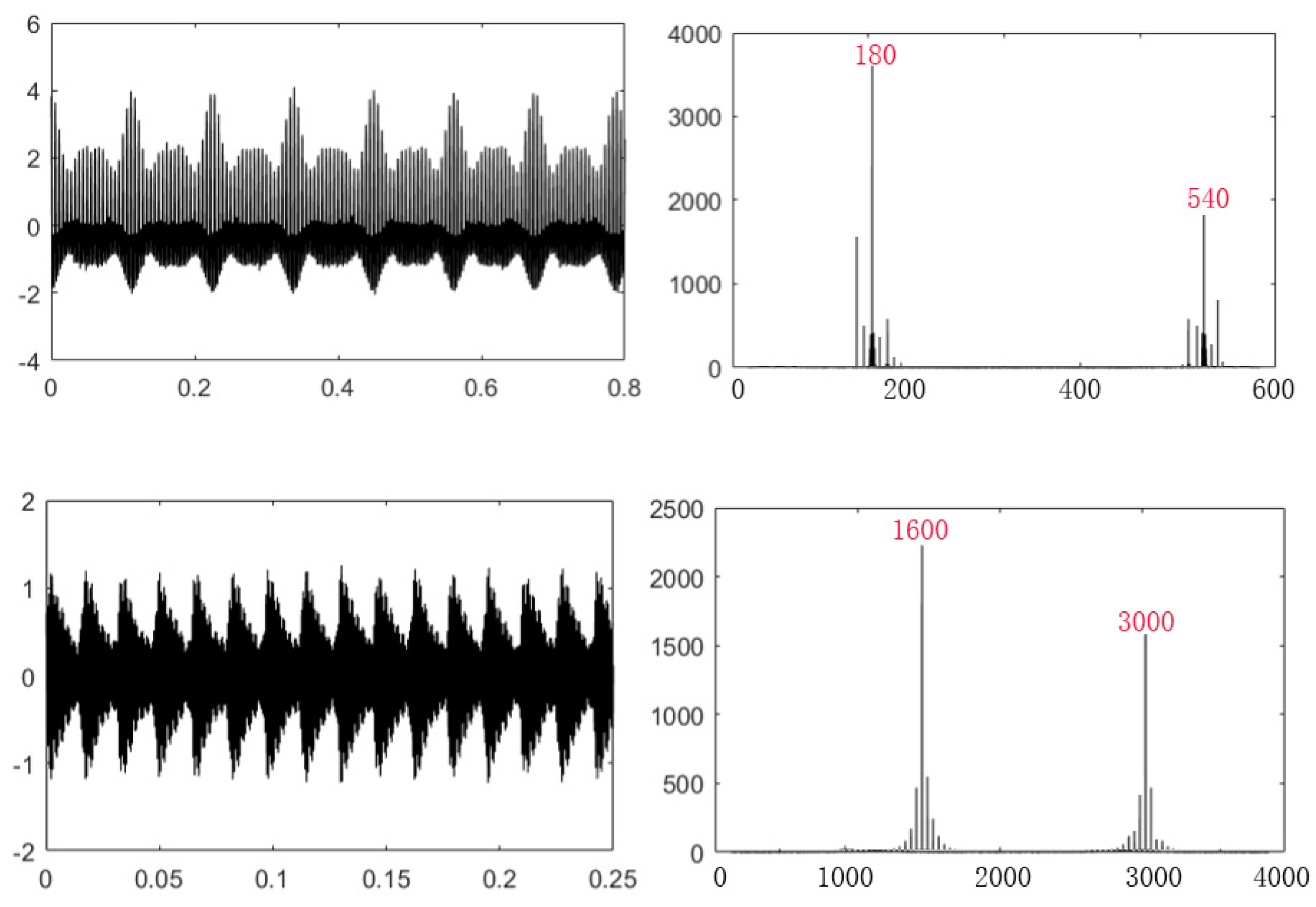
4.3. Decomposition and Reconstruction of Signals

The center frequency and bandwidth are obtained according to the optimal parameters, and the decomposed signals can be obtained by band-pass filtering of the main input signal; the decomposition results are shown in Figure 4.

For each component signal obtained by decomposition, the larger its FCFI, and the more bearing-sensitive it is. Otherwise, the component signal is considered to be insensitive. In Equation (5), N is set to 3 and $f_c$ is set to 10 for this experiment. All amplitudes of each component envelope spectrum obtained from the decomposition are arranged in descending order, and the results are shown in Figure 5.

The dashed boxes indicate the three frequency bands with a bandwidth of 10 Hz. From top to bottom of Figure 5, the calculated FCFI values for each of the four components are 0.33, 0.33, 1.83, and 1.83, respectively. It means that the latter two components contain the most bearing-related information. Therefore, the third and fourth components are reconstructed to obtain the bearing signal, and the remaining two components are reconstructed to obtain the gear signal. The results are shown in Figure 6.

It can be seen that the proposed method in this paper can effectively separate the gear-bearing composite fault signal. By observing the time domain, we can see a very obvious modulation phenomenon and shock component. From the frequency spectrum, we can clearly find the 1-fold and 3-fold engagement frequency $f_m$(180) of the gear signal, while the two resonant frequencies, $f_{c1}$(1600) and $f_{c2}$ (3000), of the bearing signal are also very clear.

4.4. Quantitative Analysis and Comparison

To further quantitatively compare the separation effect of the three methods on the composite fault signal, we introduce the average Pearson correlation coefficient [24] for judging, which is defined by the following equation:

$$\rho =\frac{1}{2}[\frac{{\sum }_{i=1}^L({x^{\prime }}_g-{{\overline{x}}^{\prime }}_g)(x_g-{\overline{x}}_g)}{\sqrt{{\sum }_{i=1}^L{({x^{\prime }}_g-{{\overline{x}}^{\prime }}_g)}^2}\sqrt{{\sum }_{i=1}^L{(x_g-{\overline{x}}_g)}^2}}+\frac{{\sum }_{i=1}^L({x^{\prime }}_b-{{\overline{x}}^{\prime }}_b)(x_b-{\overline{x}}_b)}{\sqrt{{\sum }_{i=1}^L{({x^{\prime }}_b-{{\overline{x}}^{\prime }}_b)}^2}\sqrt{{\sum }_{i=1}^L{(x_b-{\overline{x}}_b)}^2}}].$$

(15)

Larger average Pearson correlation coefficients indicate a better separation effect of methods. In Equation (15), L denotes the data length with the value of 6000. ${x^{\prime }}_g$ and $x_g$ denote the gear signal obtained by separation and the simulated original gear signal, respectively. ${x^{\prime }}_b$ and $x_b$ denote the separated bearing signals and simulated original bearing signals; ${{\overline{x}}^{\prime }}_g$, ${\overline{x}}_g$, ${{\overline{x}}^{\prime }}_b$, and ${\overline{x}}_b$ represent their mean values.

In the context of this paper, we composed three different decomposition methods, which are empirical mode decomposition (EMD) [25], VMD with parameters [3, 2000], and our variable scale adaptive decomposition method. The calculated Pearson correlation coefficients for the three methods are shown in

Table 2. Average Pearson correlation coefficients of the three methods.

	EMD	VMD Parameter as [3, 2000]	Our Method
Average Correlation Coefficient ($\rho$)	0.5232	0.4778	0.5914

. From the table, we can see that the correlation coefficients of the methods in this paper are improved, to different degrees, compared with the other two methods, which indicates better signal separation.

Furthermore, we compared the FCFI metrics of these three approaches, and the results are shown in Figure 7. From the Figure 7, we can see that the adaptive signal decomposition and reconstruction algorithm proposed in this paper obtains higher FCFI values. This result shows the superiority of our method in feature separation for gear-bearing composite fault signals, and indicates its superior differentiation of gear and bearing signals.

5. Conclusions

The fault monitoring and diagnosis of gears and rolling bearings play an important role in the health management of mechanical transmission equipment. However, the simultaneous occurrence of gear and bearing faults usually results in a composite fault signal, which makes diagnosis difficult. Therefore, we propose a variable-scale adaptive feature separation method, based on VMD and MPA algorithms, to deal with gear-bearing composite fault signals. In this method, we first use VMD to decompose the sensed composite fault signal into multiple modes. Then, we group the modes and reconstruct them into fault signals of gears and bearings. In addition, we introduce the intelligent algorithm MPA to improve feature separation ability. MPA takes the minimum kurtosis of the reconstructed signal as the optimization goal, and iteratively finds the optimal solution of the VMD parameters. Our experiments verify the convergence of the MPA algorithm and the feasibility of our decomposition and reconstruction scheme. Additionally, the superiority of our method has been verified.

References

1. Da Lpiaz, G.; Rivola, A.; Rubini, R. Effectiveness and Sensitivity of Vibration Processing Techniques. Mech. Syst. Signal Process. 2008, 10, 387–412. [Google Scholar]
2. Liu, J.; Tang, C.; Pan, G. Dynamic modeling and simulation of a flexible-rotor ball bearing system. J. VIib. Control 2021. [Google Scholar] [CrossRef]
3. Xia, C.; Wang, Z. Drivers analysis and empirical mode decomposition based forecasting of energy consumption structure—ScienceDirect. J. Clean. Prod. 2020, 254, 120107. [Google Scholar] [CrossRef]
4. Ghelardoni, L.; Ghio, A.; Anguita, D. Energy Load Forecasting Using Empirical Mode Decomposition and Support Vector Regression. IEEE Trans. Smart Grid 2013, 4, 549–556. [Google Scholar] [CrossRef]
5. Corizzo, R.; Ceci, M.; Fanaee-T, H. Multi-aspect Renewable Energy Forecasting. Inf. Sci. 2020, 546, 701–722. [Google Scholar] [CrossRef]
6. Zhang, Y.; Han, J.; Pan, G. A multi-stage predicting methodology based on data decomposition and error correction for ultra-short-term wind energy prediction. J. Clean. Prod. 2021, 292, 125981. [Google Scholar] [CrossRef]
7. Ceci, M.; Corizzo, R.; Japkowicz, N. ECHAD: Embedding-Based Change Detection from Multivariate Time Series in Smart Grids. IEEE Access 2020, 99, 156053–156066. [Google Scholar] [CrossRef]
8. Aubras, F.; Damour, C.; Benne, M. A Non-Intrusive Signal-Based Fault Diagnosis Method for Proton Exchange Membrane Water Electrolyzer Using Empirical Mode Decomposition. Energies 2021, 14, 4458. [Google Scholar] [CrossRef]
9. Soualhi, A.; El Yousfi, B.; Razik, H.; Wang, T. A Novel Feature Extraction Method for the Condition Monitoring of Bearings. Energies 2021, 14, 2322. [Google Scholar] [CrossRef]
10. Dragomiretskiy, K.; Zosso, D. Variational Mode Decomposition. IEEE Trans. Signal Process. 2014, 62, 531–544. [Google Scholar] [CrossRef]
11. Daubechies, I.; Lu, J.; Wu, H. Synchrosqueezed wavelet transforms: An empirical mode decomposition-like tool. Appl. Comput. Harmon. Anal. 2010, 30, 243–261. [Google Scholar] [CrossRef] [Green Version]
12. Huang, S.; Sun, H.; Wang, S. SSWT and VMD Linked Mode Identification and Time-of-Flight Extraction of Denoised SH Guided Waves. IEEE Sens. J. 2021, 21, 14709–14717. [Google Scholar] [CrossRef]
13. Zhong, J.; Gou, X.; Shu, Q. A FOD Detection Approach on Millimeter-Wave Radar Sensors Based on Optimal VMD and SVDD. Sensors 2021, 21, 997. [Google Scholar] [CrossRef]
14. Zhang, H.; Liu, D. Bearing Fault Diagnosis Based on BFA Optimized VMD Parameters. Modul. Mach. Tool Autom. Manuf. Tech. 2020, 555, 50–56. [Google Scholar]
15. Shanshan, W.; Guobing, H.; Bing, G. Variational Mode Decomposition(VMD) Based Method of Leakage Locating in Water Delivery Lines. Sensor Lett. 2016, 14, 846–851. [Google Scholar] [CrossRef]
16. Soman, K.P.; Poornach, P.; Athira, S. Recursive Variational Mode Decomposition Algorithm for Real Time Power Signal Decomposition. Procedia Technol. 2015, 21, 540–546. [Google Scholar] [CrossRef] [Green Version]
17. Yuan, Z.; Zhou, T.; Liu, J. Fault Diagnosis Approach for Rotating Machinery Based on Feature Importance Ranking and Selection. Shock Vib. 2021, 2021, 8899188. [Google Scholar] [CrossRef]
18. Sahani, M.; Dash, P.K. Variational mode decomposition and weighted online sequential extreme learning machine for power quality event patterns recognition. Neurocomputing 2018, 310, 10–17. [Google Scholar] [CrossRef]
19. Mirjalili, S.; Mirjalili, S.M.; Lewis, A. Grey Wolf Optimizer. Adv. Eng. Softw. 2014, 14, 46–61. [Google Scholar] [CrossRef] [Green Version]
20. Faramarzi, A.; Heidarinejad, M.; Mirjalili, S. Marine Predators Algorithm: A Nature-inspired Metaheuristic. Expert Syst. Appl. 2020, 152, 77–104. [Google Scholar] [CrossRef]
21. Viswanathan, G.M.; Buld, S.V. Optimizing the success of random searches. Nature 1999, 401, 911–914. [Google Scholar] [CrossRef] [PubMed]
22. Bartumeus, F.; Catalan, J.; Fulco, U.L. Optimizing the Encounter Rate in Biological Interactions: Lévy versus Brownian Strategies. Phys. Rev. Lett. 2002, 88, 16–19. [Google Scholar] [CrossRef] [PubMed]
23. Amarnath, M.; Krishna, I.R.P. Empirical mode decomposition of acoustic signals for diagnosis of faults in gears and rolling element bearings. IET Sci. Meas. Technol. 2012, 6, 279–287. [Google Scholar] [CrossRef]
24. Nahler, G. Pearson Correlation Coefficient; Springer: Vienna, Austria, 2009; Volume 1025, p. 132. [Google Scholar]
25. Huang, N.E.; Shen, Z.; Long, S.R. The empirical mode decomposition and the Hilbert spectrum for nonlinear and non-stationary time series analysis. Proc. Math. Phys. Eng. Sci. 1998, 454, 903–995. [Google Scholar] [CrossRef]
Figure 1. The overall framework diagram of the multi-scale adaptive signal decomposition reconstruction method.
Energies 14 07702 g001
Figure 2. Composite fault simulation signal.
Energies 14 07702 g002
Figure 3. The convergence result of the MPA algorithm.
Energies 14 07702 g003
Figure 4. The results of VMD decomposition.
Energies 14 07702 g004
Figure 5. Envelope spectrum of component signals.
Energies 14 07702 g005
Figure 6. Reconstructing signal time domain waveforms and spectra. (Top) gear signals; (Bottom) bearing signals.
Energies 14 07702 g006
Figure 7. Comparison of FCFI metrics for the three methods.
Energies 14 07702 g007