Heat Flux Based Optimization of Combined Heat and Power Thermoelectric Heat Exchanger

Abstract

We analyzed the potential of thermoelectrics for electricity generation in a combined heat and power (CHP) waste heat recovery system. The state-of-the-art organic Rankine cycle CHP system provides hot water and space heating while electricity is also generated with an efficiency of up to 12% at the MW scale. Thermoelectrics, in contrast, will serve smaller and distributed systems. Considering the limited heat flux from the waste heat source, we investigated a counterflow heat exchanger with an integrated thermoelectric module for maximum power, high efficiency, or low cost. Irreversible thermal resistances connected to the thermoelectric legs determine the energy conversion performance. The exit temperatures of fluids through the heat exchanger are important for the system efficiency to match the applications. Based on the analytic model for the thermoelectric integrated subsystem, the design for maximum power output with a given heat flux requires thermoelectric legs 40–70% longer than the case of fixed temperature reservoir boundary conditions. With existing thermoelectric materials, 300–400 W/m² electrical energy can be generated at a material cost of $3–4 per watt. The prospects of improvements in thermoelectric materials were also studied. While the combined system efficiency is nearly 100%, the balance between the hot and cold flow rates needs to be adjusted for the heat recovery applications.

1. Introduction

Up to two thirds of primary energy is unused or rejected in the U.S. [1] and worldwide [2]. Most of the energy loss is in the form of heat, which is the lowest quality of energy [3]. Minimizing this loss will save energy and help reduce the impact of global warming. A significant amount of heat energy is required for industry. For example, material processing involves large heat generation through furnaces, e.g., for melting glass [4] and steel [5], or electromagnetic heating for aluminum [6]. Most of the heat is rejected in the gas phase, e.g., with air, which minimizes the complexity of controlling the temperature of the process. The waste heat recovery system should extract useful energy from this hot gas. In the industrial sector, which consumes nearly a quarter of the total energy resources, the waste heat temperature distribution was reported in 2008 [7]; more than 54% of waste heat is in the temperature range of 100–200 °C, followed by more than 21% in the 200–300 °C temperature range (see Figure 1; a more detailed distribution is also shown in the reference pie chart [7]). Similar data are reported for European industries [8]. Large amounts of heat energy are rejected from automotive internal combustion engines as well as from furnaces in residential and commercial sectors. Most likely, the waste heat temperatures are in a similar range. This is because the combustion for chemical energy conversion has flame temperatures of over 1000 °C, up to about 2000 °C [9] under adiabatic combustion conditions, with an air mixing volumetric ratio of more than 1:10. Hence, we set the temperature of waste heat to 100–300 °C in this investigation [10].

Thermodynamically, low temperatures are not very desirable for full conversion into electricity, as exergy loss is relatively large compared to high temperature applications [11]. The combined heat and power (CHP) system represents a highly efficient pathway for waste heat energy recovery by providing heat with useful temperatures simultaneously. There are numerous heating needs in residential and commercial buildings. Especially in cold climate zones, such as northern Europe, some cities and towns are already built with hot air/water supply networks from large industrial factories. In this paper, we analyze a smaller-scale CHP system from a heat input of up to 1000 kW. Mechanical thermodynamic power generators have a limitation with respect to scaling down due to the increased heat loss as the surface-to-volume ratio increases. Among the variety of thermodynamic energy conversion technologies [12], especially for CHP systems with a relatively low temperature heat source, organic Rankine cycles (ORCs) have been intensively studied. For example, dynamic modeling of ORC [13] and experimental investigation for ceramic processes [14] have been performed. The efficiency of an ORC with a variety of working fluids was reported as 12% from a heat source of 1.3 MW_thermal at 145 °C [15]. However, the smaller the scale, the lower the efficiency. Uusitalo et al. [16] summarized the systematic test results of smaller-scale ORCs with a recuperation system rated at 67 kW_thermal input at 250 °C, which generated 3.2–5.9 kW (net efficiency of 4.2–7.7%). Therefore, we have investigated a novel CHP integrated thermoelectric system, which is scalable under 100 kW_thermal. One such example is residential heating applications.

The efficiency at the maximum power output of typical commercial thermoelectric generators is slightly over 5% with today’s non-dimensional material figure of merit (ZT), which is unity. The value is determined by $Z=\sigma S^2/k$, where $\sigma$ is electrical conductivity, $S$ is the Seebeck coefficient, and $k$ is thermal conductivity. T is the absolute temperature. The overall system efficiencies can be comparable with ORCs at this scale or smaller, according to our model [17]. In addition, thermoelectric modules have a flexible design and are distributed in nature. They allow integration inside heat exchangers and local optimization in a way that is not possible with ORCs or other thermodynamic engines. Considering the above, we explore the potential of thermoelectric energy conversion to generate power, along with heat for hot water supply and space heating. Optimizing the system for low temperature heat is important. We optimize the thermoelectric integrated heat exchanger subsystem and then discuss the applicability of the temperature range, which is a result of the design, but could be expanded in the future. The thermoelectric materials are simply considered as commercially available bismuth telluride (Bi₂Te₃) with ZT = 1. We use the logarithmic mean temperature difference (LMTD) between the two fluids, which is very commonly implemented during the design of heat exchangers and is useful for determining the “mean” performance of the heat exchanged between the fluids.

2. Materials and Methods

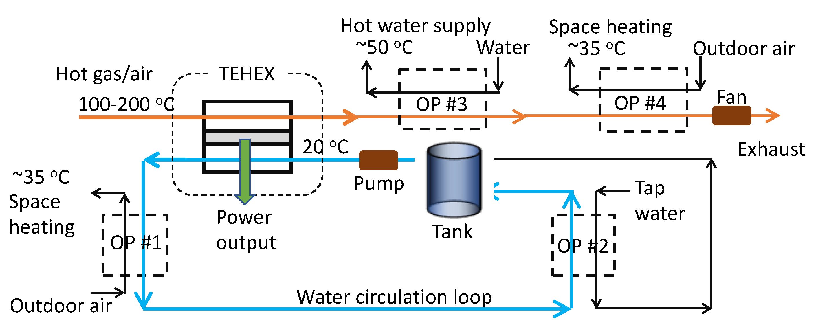
2.1. CHP System

The CHP system in this study is relatively small scale, with a heat source of a few 100 kW. In realistic systems, the feeding temperature of waste heat is a variable and not strictly given. The origin of the waste heat is a constant temperature combustion process, which means virtually infinite heat capacity. However, this is not the case for practical waste heat recovery systems. Instead, we must consider a given heat flux condition, hence the changes in the temperature of feeding hot gas depending on the thermal resistance of the downstream (drain) to the thermal ground. The heat flux can change depending on the upstream process, but we consider a quasi-steady state and we do not consider the dynamic response in this work. In order to analyze the performance with such boundary conditions, we investigated a heat flux-based model for thermoelectric (TE) integrated heat exchanger where the output hot gas and liquid is another source of heat energy. The ideal overall CHP system is shown in Figure 2.

In a distributed CHP system, the output power may likely be consumed locally. Hot water or gas pipelines are important for systems in buildings or at the community scale [18]. The cost and optimization of the heat energy distribution will be discussed in future work. We expect utilization of the CHP system for smaller-scale industrial processes in addition to residential and commercial buildings. There are many smaller-scale manufacturing facilities around the world, including in many developing countries. We expect this technology to be adaptable as a bottoming cycle to the exhaust heat harvesting from fuel-burning mechanical thermodynamic systems.

2.2. Thermoelectric Integrated Subsystems

The thermoelectric integrated heat exchanger subsystem (see Figure 3) is a key part of the above CHP system. Unlike commercial off-the-shelf thermoelectric modules, the subsystem does not have ceramic plates that hold the thermoelectric legs. Instead, channeled heat conduction plates hold the legs, with electrical insulator layers and printed/laminated interconnects. There are studies [19] on the direct mount of TE legs on the microchannel cold plate to minimize the interface thermal resistances to improve the heat transfer. The fundamental idea is the same, but this integrated subsystem is designed to co-optimize the total heat and power energy harvesting performance. This requires the design and local optimization of thermoelectric legs that varies with the hot-side gas flow and the cold-side water flow as the core of the CHP system.

In the following investigation, the electrical load connected to the TE system is always optimized. Electrical load must be adjusted to the input conditions, similarly to the maximum power point tracker [20] circuitry for photovoltaics. The matched load for finite thermal resistance with constant temperature heat source and heat sink is $R_{TE}\times \sqrt{1+ZT}$, where $R_{TE}$ is the intrinsic electrical resistance of the TE subsystem [21]. The internal resistance includes a total series resistance of legs, contacts, and electrical interconnects.

Temperatures across the subsystems are determined based upon the heat energy flow balance, as shown in the following. Note that all the energy and power terms are per unit area. In the hot-side gas flow, noted by subscript $g$, we have

$$Q_{g,in}={\dot{m}}_{g}C{p}_g\left(T_{g,in}-T_{g,out}\right)$$

(1)

$$Q_{g,out}={\dot{m}}_{g}C{p}_g\left(T_{g,out}-T_a\right)$$

(2)

In the cold-side water flow, noted by subscript $w$, we have

$$Q_{w,in}={\dot{m}}_{w}C{p}_w\left(T_{w,in}-T_a\right)$$

(3)

$$Q_{w,out}={\dot{m}}_{w}C{p}_w\left(T_{w,out}-T_{w,in}\right)$$

(4)

where $T_a$ is the ambient air temperature, which is the ultimate heat sink. It is also the temperature of tap water flowing into the system, considering that it is equal to the ambient temperature. The temperatures $T_g$ and $T_w$ are not equal to the hot- and cold-side temperatures of the thermoelectric legs, respectively. At each leg, a difference in temperature occurs due to the convective heat transfer from the fluid to the solid or vice versa. It is common to expect a logarithmic temperature gradient along the channels on both sides. An approximation can be found in heat transfer textbooks [22]. The power generated from thermoelectric conversion is a function of $T_h$ and $T_c$, which are the temperatures at the terminal nodes of a thermoelectric leg.

$$P_{TE}=N\frac{m\sigma S^{2}FA}{\left(1+m\right)d}\left(T_h-T_c\right)$$

(5)

where $N$ is the number of legs per unit area, $F$ is the fill factor, $A$ is the footprint area of the thermoelectric module, $d$ is the leg length, $\sigma$ is electrical conductivity, and $S$ is the Seeback coefficient. Here, $m$ is the ratio of external load over the internal resistance of the subsystem, and the optimum ratio for the maximum power output is determined as $m=\sqrt{1+ZT}$ for the thermoelectric factor, the same as for the electrical load matching factor [17]. This equation simply follows Ohm’s law with internal potential generation due to $V=S\left(T_h-T_c\right)$ for the thermoelectric leg.

We need to determine a set of fluid intermediate temperatures, which are the basis for heat transfer via convection or radiation with the channel wall. These are directly connected to the terminal temperatures. In order to investigate the simplest one-dimensional (1D) heat transfer, $T_h$ and $T_c$ are considered to be the representative temperatures of the hot- and cold-sides of the numerous legs, respectively ($N$ per unit area). An immediate challenge that can be noticed is that the fluid intermediate temperature must be quantified first to find $T_h$ and $T_c$. However, these are changed by the active thermal resistance through the thermoelectric leg when power is generated. Therefore, the temperature network must be solved iteratively until the energy balance is found. The temperature profile along the distance across the channel follows a natural logarithmic function. The log mean temperature difference (LMTD) is determined as

$$LMTD=\frac{\left(T_{g,in}-T_{w,out}\right)-\left(T_{g,out}-T_{w,in}\right)}{ln\left(T_{g,in}-T_{w,out}\right)-ln\left(T_{g,out}-T_{w,in}\right)}$$

(6)

$$T_{g,m}=T_{w,m}+LMTD$$

(7)

The modeled thermal profile in the thermoelectric integrated heat exchanger is shown in Figure 4. The total waste heat energy is determined by the temperature difference $\left(T_{g,in}-T_{w,in}\right)$.

Then, the convective heat transfer between the fluid and the wall is given as

$$Q_{TE,in}=h_{h,eff}\left(T_{g,m}-T_h\right)$$

(8)

$$Q_{TE,out}=h_{c,eff}\left(T_c-T_{w,m}\right)$$

(9)

where $h$ is effective heat transfer coefficient between the intermediate fluid temperature and the solid wall of channel. This coefficient is mainly a convective term but can include a non-liner radiation term if the absolute temperature is very large.

$$h_{eff}=h_{conv}+\sigma {\epsilon }_R{V}_f\left|\left(T_{fluid}{}^2-T_{wall}{}^2\right)\right|\left(T_{fluid}+T_{wall}\right)$$

(10)

$$h_{conv}=\frac{k_f}{D_h}Nu$$

(11)

where $\sigma$ is the Stefan–Boltzmann constant, ${\epsilon }_R$ is emissivity of radiation heat transfer, $V_f$ is the view factor, $k_f$ is thermal conductivity of the fluid, $D_h$ is the hydraulic diameter, and $Nu$ is the Nusselt number. In this work, we used the Sieder–Tate correlation [23] for the volumetric mean of fluid flow.

$$h_{conv}=\frac{k_f}{D_h}Nu$$

(12)

where $Pr$ is the Prandtl number of the fluid, $\frac{\mu }{{\mu }_w}$ is the ratio of viscosities of the bulk fluid to that of the section near the wall (for considering the temperature dependency), and $Re$ is the Reynolds number. This correlation is valid for both gas and water for sufficiently long channels and $Re>\mathrm{10,000}$.

$$Re=\rho \frac{D_h}{\mu }\frac{\dot{m}}{A_{ch}}$$

(13)

where $\rho$ is the density of fluid, $A_{ch}$ is the cross-sectional area of the channel, and $\dot{m}$ is the mass flow rate of the fluid. Due to the smaller cross section of the channels relative to the channel length on both sides, the flow regime and heat transfer characteristics follow the microchannel or minichannel heat transfer, which is considered to be fully developed flow.

From a system perspective, the energy recovered by heat convection in the subsystem from the hot gas is

$$E=\epsilon Q_{w,out}+P_{TEG}$$

(14)

where $Q_{w,out}$ is the drainage heat at a lower temperature that still remains a usable temperature for something else, $\epsilon$ is the effectiveness of the thermoelectric integrated heat exchanger, and $P_{TEG}$ is electrical power as the output of the thermoelectric generator. The energy supplied to the subsystem is $Q_{g,in}$. Therefore, the energy harvesting efficiency is given by

$$\eta =\frac{E}{Q_{g,in}}$$

(15)

The total energy that comes out from the subsystem must conserve the energy input. Therefore,

$$Q_{g,in}=\epsilon Q_{w,out}+Q_{g,out}+P_{TEG}$$

(16)

The exhaust gas from heat exchange $Q_{g,out}$ can be considered as being one of the heat energy outputs and a potential source of useful thermal energy. This gas exit temperature must satisfy the usable threshold $T_{g,usable}$:

$$T_{g,out}\ge T_{g,usable}$$

(17)

In this special case, the efficiency becomes

$$\eta =\frac{E^{\prime }}{Q_{g,in}}=\frac{\epsilon Q_{w,out}+Q_{g,out}+P_{TEG}}{Q_{g,in}}$$

(18)

As long as $T_{g,out}$ satisfies the threshold, the effectiveness of the heat exchanger can be smaller while maximizing $P_{TEG}$. If not, it is quite important to balance the effectiveness between the heat and electrical energy harvesting mix, depending on the electricity demand for the application.

The $P_{TEG}$ described here is equal to the intrinsic power out from the thermoelectric legs in the subsystem. However, for the whole CHP system, a tradeoff due to the power consumption of the fan ($P_{FAN}$) and the pump ($P_{PUMP}$) must be taken into account. Such power is necessary to obtain a certain level of energy harvesting performance.

$$P_{net}=P_{TEG}-P_{FAN}-P_{PUMP}$$

(19)

This net power output ($P_{net}$) replaces ($P_{TEG}$) in the above equation when the whole CHP is considered.

2.3. Working Fluids

Water is desirable as a working fluid in general since it has a large heat capacity to transfer the heat by mass transport. Conveniently, we can use tap water for the cold side to warm up the working fluid for use in space heating with or without a combined thermal storage tank. Furthermore, its higher thermal conductivity relative to the gases helps to make the heat exchanger compact. Regarding the energy payback by introducing fluid movers (fan and pump), the pump power is nearly proportional to the cube of flow rate, which is also proportional to the density and the kinematic viscosity. The fluid dynamic power is a product of pressure loss and volumetric flow rate, where pressure loss is mostly caused by wall friction with velocity square. Considering a circular pipe and pure laminar flow, the performance of heat transfer Q against the input fluid dynamic work W can be determined as Equation (20) below. The larger the value, the better the waste heat recovery applications. The last term in the equation only consists of fluid properties (k—thermal conductivity, C_p—specific heat, $\rho$—density, and $\nu$—viscosity), which we took as an index to compare various fluids. Clearly, water is a preferable fluid for a good payback time with high heat energy transfer. In comparison, Fluorinert FC72 (a fluorocarbon which is a popular working fluid for cooling electronics) has an index of 28.5 at 25 °C, as calculated from the specification data [24]. It is beneficial that the index for water increases at higher temperatures, but its use is limited at the cold side before boiling. Therefore, water is not suitable for the hot side. Air is abundantly available and requires no special high-cost hermetic seal, no concern for toxicity for safety, nor requires large pressures to maintain the properties. Therefore, we investigated the performance of the system with air for the hot-side fluid as the reference.

$$\frac{Q}{W}=\frac{C}{2}{\left(\frac{D_h{}^2}{u^3}\right)}^{0.4}{\left(\frac{k{C}_p{}^2}{\rho {\nu }^{4.4}}\right)}^{1.333}$$

(20)

In

Table 1. Fluid properties and heat transfer performance indexes.

	Temperature	Density	Specific Heat	Thermal Conductivity	Viscosity	Performance Index	Relative Index
	°C	kg/m3	J/(kg·K)	W/(m·K)	×10−6 m2/s
Air	20	1.166	1005	0.0257	15.6	3.16 × 108	1.00
	160	0.789	1017	0.0359	30.8	1.49 × 108	0.47
Steam	160	0.494	1984	0.0286	29.7	2.67 × 108	0.84
Water	20	998.2	4181	0.594	1.01	1.36 × 1010	43.0
	40	992.3	4177	0.628	0.667	2.54 × 1010	80.6
	60	983.2	4186	0.653	0.481	4.18 × 1010	132.5
	80	971.8	4198	0.672	0.367	6.32 × 1010	200.1

, these related typical material properties are summarized.

A moderate temperature is considered for the hot gas, in a range of 100–300 °C. The analytic model is applicable regardless of temperature regime, while properties of the fluid should be carefully chosen. For the hot-side heat transport, a working fluid at such a temperature is really challenging and cost ineffective; hence, gas is the natural selection. Convection heat transfer between the gas to the solid wall is much weaker than that of the cold-side water, as the thermal conductivity is much smaller. Hence, the hot-side heat transfer is most likely the limiting component of the heat energy flow through the subsystem, hence limiting the generation of thermoelectric power.

2.4. Thermoelectric Materials

The above imbalance between the hot- and cold-side thermal contacts will push the temperature profile across the thermoelectric leg to the lower side for maximum power output. In general, the temperature difference between the two nodes does not change as much as changing the asymmetric ratio, while the conversion efficiency changes due to the thermodynamic nature. The intrinsic energy conversion efficiency is given by

$$\eta =\left(1-\frac{T_c}{T_h}\right)\left(\frac{\sqrt{1+ZT}-1}{\sqrt{1+ZT}+\frac{T_c}{T_h}}\right)$$

(21)

If the same temperature difference across the leg remains, the efficiency increases slightly as the temperatures decrease. Hendricks et al. made the argument [25] that the ideal ratio of asymmetricity is around 10–20 times for conductance of the cold side against the hot side. Therefore, the hot-side fluid can conveniently be air or a mixed flue gas.

Considering that the mean temperature across the leg is the reference temperature of the material performance, the best thermoelectric material for this condition should have a ZT peak near the quarter of temperature difference, $T_{ref}\approx T_g+\left(T_g-T_w\right)/4$, or slightly lower than that. For example, if the heat source is 200 °C, the temperature of the ZT peak will be around 65 °C when the thermal heat sink is 20 °C. Therefore, among the available thermoelectric materials, Bi₂Te₃ reasonably fits this requirement, with a ZT of more than 1.0 (both for p-type and n-type), and is widely available in the market. In the following analyses, we used the temperature-independent material properties (absolute value) for the thermoelectric legs of both n-type and p-type. The values are as follows: Seebeck coefficient, 2.4 × 10⁻⁴ V/K; electrical conductivity, 1.5 × 10⁵ 1/($\mathsf{\Omega }$·m); and thermal conductivity, 3.0 W/(m·K). With a temperature of 74 °C, the ZT value is 1.0. Note that due to the fixed Z value, the ZT value is slightly larger at a higher temperature. In the cost and power analysis, potential material properties (ZT = 1, 2, 3 by changing the power factor or thermal conductivity) are considered for potential performance with future enhanced materials. However, the material prices are assumed to be the same as current ones. Bi₂Te₃ is inherently an expensive raw material, costing as much as $500/kg.

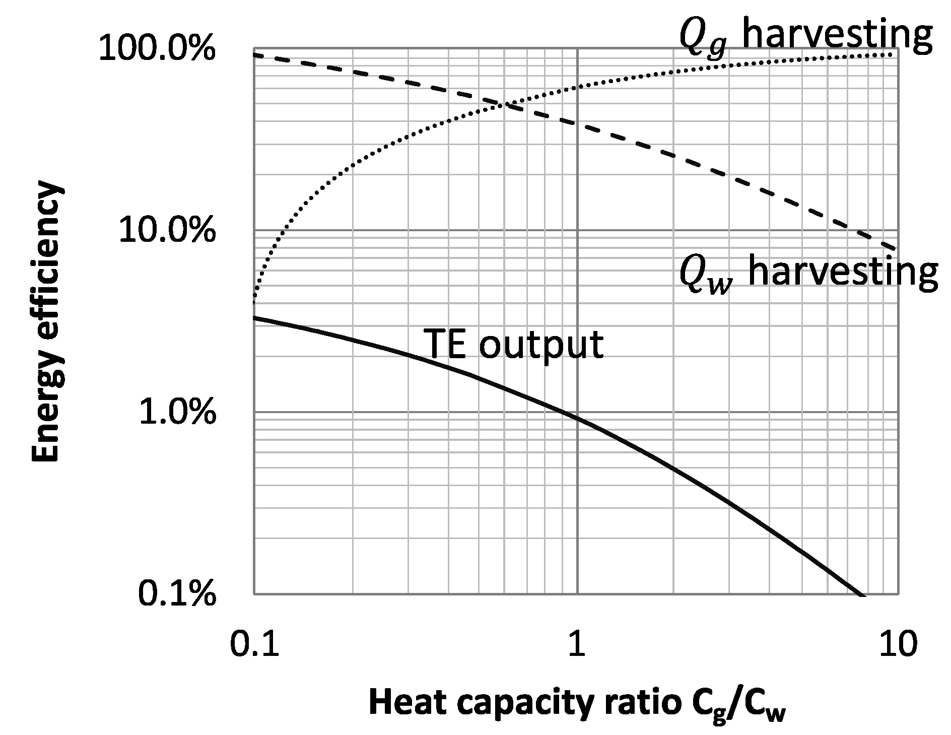
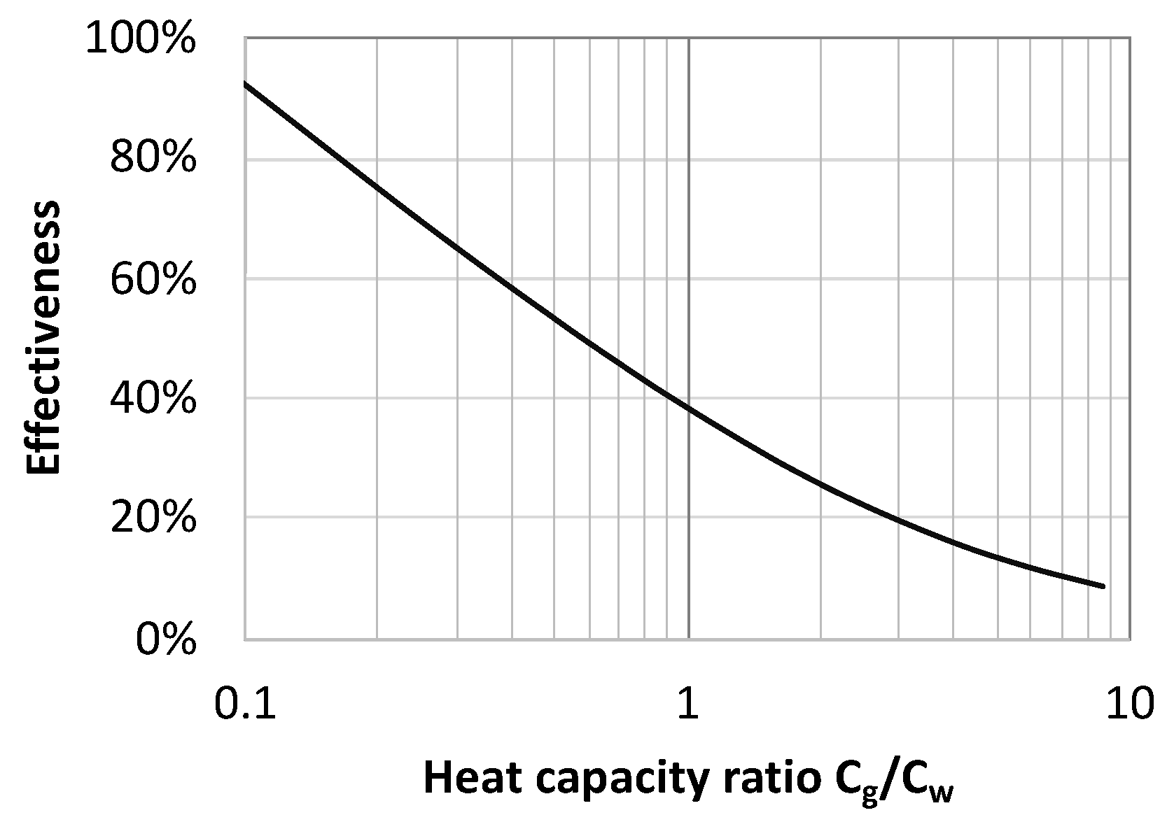
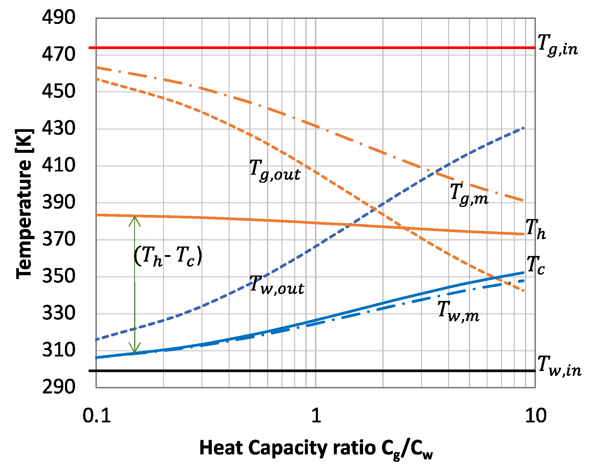
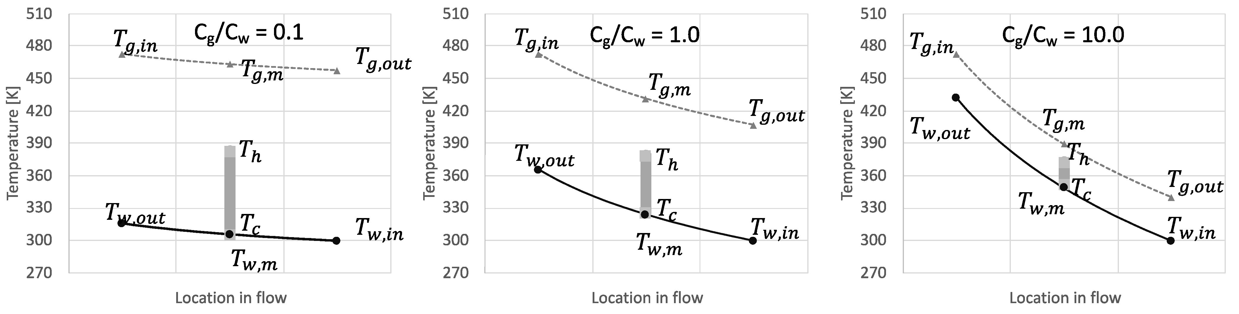
2.5. Effectiveness of Heat Exchanger

The heat transfer effectiveness of the thermoelectric integrated heat exchanger is an important measurement, as the outlet heat contained in the working fluids will be used in the downstream. This is particularly important, as the CHP system has a focus on the water temperature. A big assumption for the calculations is that heat energy removal through the thermoelectric conversion process is a fraction of the heat flow and could be negligible. This helps to eliminate the complexity. The conversion efficiency at the maximum power output (for the cost effectiveness) is 7.5% or less, so the assumption should be reasonable. The effectiveness (ε) is defined as the ratio between the heat capacities of hot- and cold-fluid flow.

$$\epsilon =\frac{\left(T_{w,out}-T_{w,in}\right)}{\left(T_{g,in}-T_{w,in}\right)}\frac{C_w}{C_g}$$

(22)

where $C_g$ and $C_w$ are heat capacity of the gas and water flow, respectively, determined by $C_g={\dot{m}}_{g}C{p}_g$ and $C_w={\dot{m}}_{w}C{p}_w$. Because of the significantly different properties, the channel diameter is designed differently. Including some reasonable design for manufacturing, we used channel dimensions of 2 mm diameter for the water passage and 10 mm diameter for the gas passage.

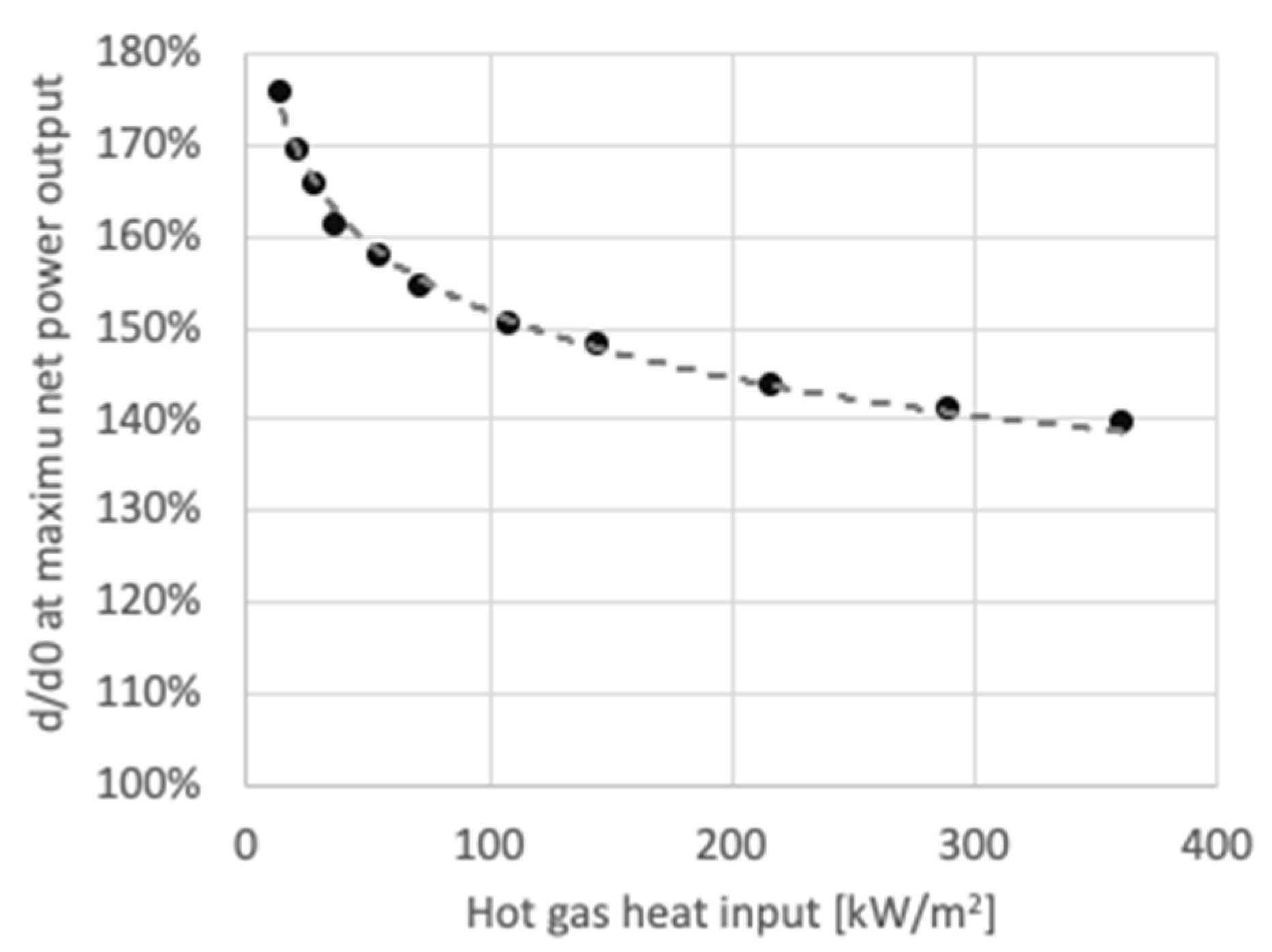
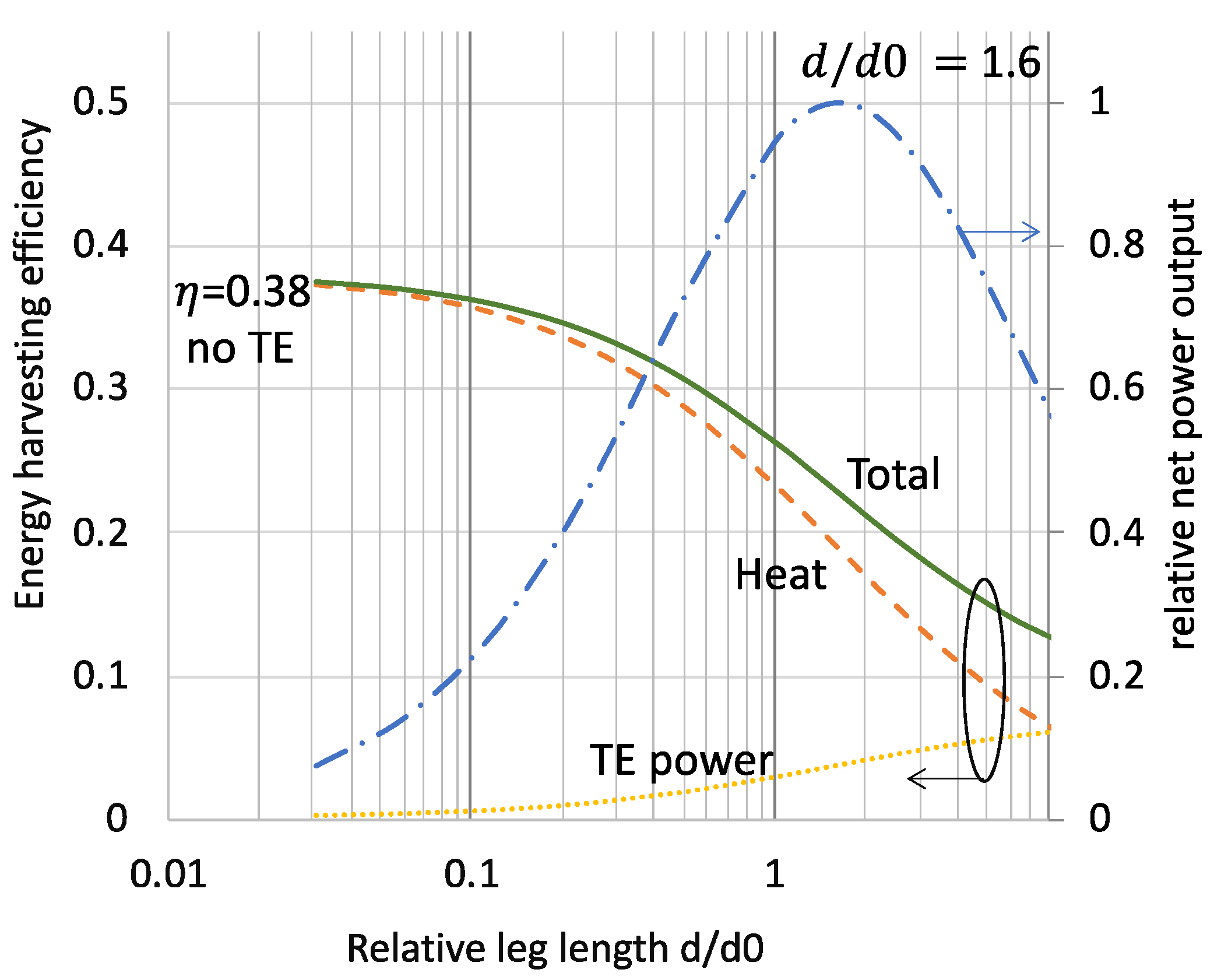
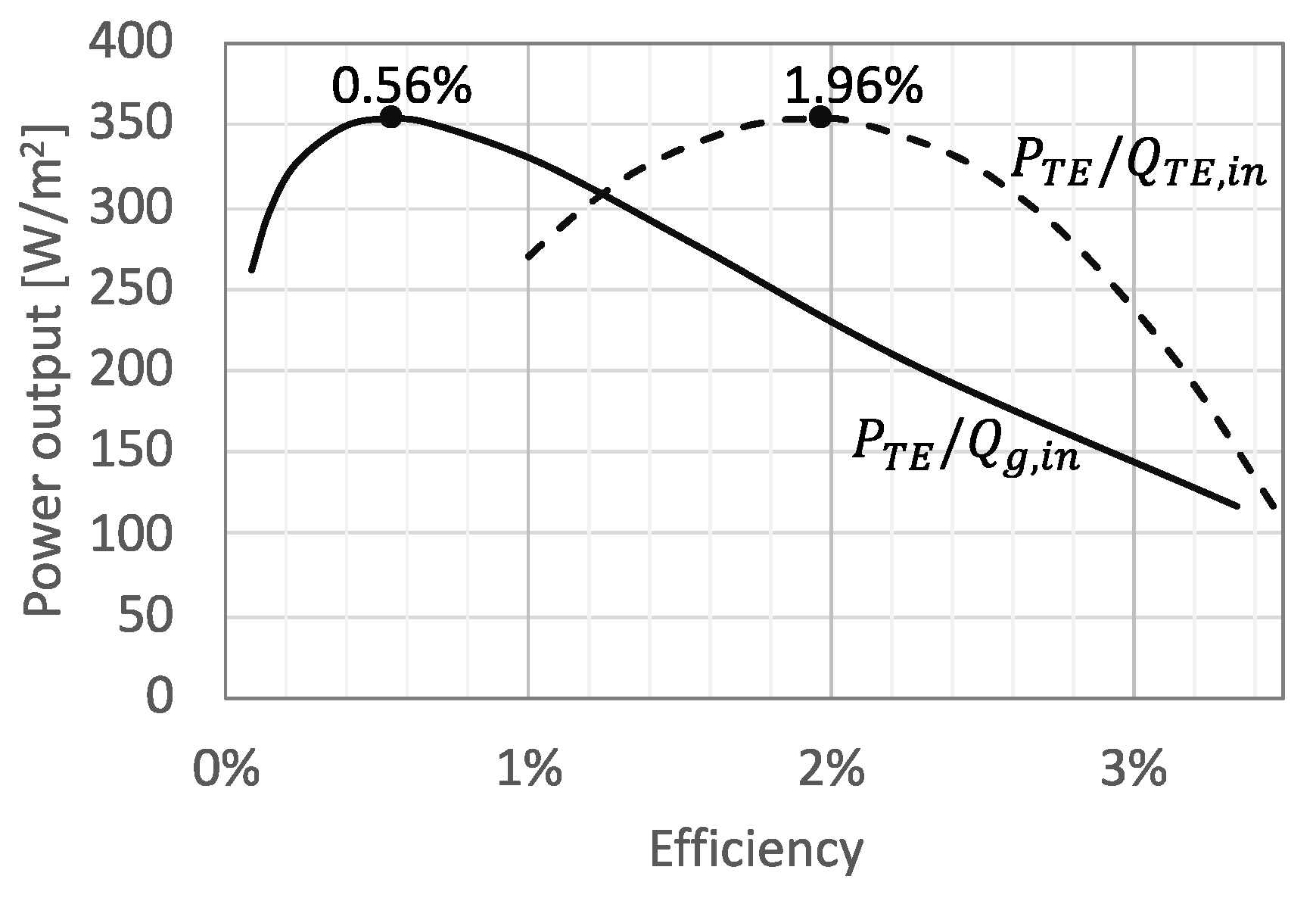
2.6. Thermoelectric Optimum Design

The length of the thermoelectric elements (legs) has been optimized with respect to a fixed cross-section area of 0.1 mm², with a fill factor of 10% and 1 × 10⁶ elements per 1 m². Relatively, this fill factor number is aggressively small, but it is helpful for a cost effective solution in addition to lowering the profile of the thermoelectric integrated heat exchanger. The optimum leg length for the maximum power output [26] can be determined as

$$d_{opt}=\frac{4}{{\alpha }^2}mkFA{\displaystyle \sum }\psi$$

(23)

where $k$ is the thermal conductivity, $F$ is the fill factor, $A$ is the cross-sectional area of the thermoelectric leg, and the thermal resistance $\psi$ at both the hot and cold terminals is calculated from the heat transfer coefficients. The variable $\alpha$ is the asymmetric factor of the thermal system; $\alpha =2$ when the system is perfectly symmetric. In the studied case, the system was highly asymmetric, as the ratio of the hot-side thermal resistance to that of the cold side ranged from 10 to several 100, depending on the flow rate. The $\alpha$ value varies between 1.95 and 1.99, according to the ratio. This factor is considered to be an insignificant factor and has thus been excluded from the results. The key investigation in this work is that the temperature at the node is not fixed, but a function of fluid flow.

2.7. Uncertainty

The sources of uncertainty for performance prediction lie in the material properties, especially their temperature-dependent characteristics, heat transfer coefficients, and some geometry-dependent properties such as contact interface resistance inside the thermoelectric module. In addition, the factors not taken into account in the presented analysis are the tolerance and allowance of manufacturing. As the physical device and the system have been designed with respect to a specific manufacturing process, the potential uncertainty can be determined.

3. Results and Discussion

3.1. Performance Analysis

An analytic thermoelectric performance model following Ref. [17] was used to evaluate the performance of the thermoelectric integrated heat exchanger subsystem. The calculation was conducted for a 200 °C heat source supplied by the mass flow of gas, as this is typical. As aforementioned, however, the temperature gradient across the thermoelectric legs is not given because the accessible fluid temperature changes according to flow rate and is partially converted to electricity. The heat input and output are constrained by the source and the sink heat capacities, which are the product of mass flow rate and specific heat. In order to identify an economically meaningful solution, we pursued the design for maximum power output. Figure 5 shows the ratio of the leg length relative to the one at maximum power output with fixed node temperatures. It can be seen that in the case of heat flux boundary conditions, the legs are longer than those for fixed-temperature reservoirs. The ratio changes depending on the hot-side heat input as the cold-side flow rate is kept constant. Figure 6 shows a detailed analysis of the impact of design (leg length) at the matched heat capacity between the hot gas and cold water ($C_g=C_w).$ A value of $d/d0=0$ virtually corresponds to a case of a heat exchanger without thermoelectric legs in place.

Figure 7 shows the potential energy harvesting from the two heat outputs (water and gas) as well as the thermoelectric power. In practice, different energy harvesting options need to be optimized. The thermoelectric module enables electrical power when it is needed, and the heat output must match the temperature of the application, such as water boiler or space heating, etc.

As we change the heat capacity ratio between the water and gas channels by changing the water flow rate alone, the power output and efficiency change (Figure 8).

With this behavior, there are two definitions of efficiency (Figure 9). The smaller efficiency is the one we already defined with Equation (15), which determines the power generation performance of the thermoelectric integrated heat exchanger. The other is an intrinsic conversion efficiency which only considers the heat flow through the thermoelectric legs. This is most often used as the thermoelectric subsystem conversion efficiency.

In this configuration, the peak power is observed at $Q_{g,out}$ equal to 71% of $Q_{g,in}$. As a heat exchanger, the performance of heat transfer by contacting two fluids is measured by effectiveness [27], which can be found in the heat exchanger books as

$$\epsilon =\frac{T_{w,out}-T_{w,in}}{T_{g,in}-T_{w,in}}\frac{C_w}{C_g}$$

(24)

This is an index of what ratio of heat is extracted through contact via a thermally conductive separator. Figure 10 shows the effectiveness as a function of the ratio of the heat capacities in the hot gas and cold water channels. From an experimental perspective, the effectiveness is also given by

$$\epsilon =\frac{T_{g,out}-T_{g,in}}{T_{g,in}-T_{w,in}}\frac{C_g}{C_g}=\frac{T_{g,in}-T_{g,out}}{T_{g,in}-T_{w,in}}$$

(25)

This number is used to determine whether the exhaust gas is valuable for harvesting the contained heat. Based on the second law of thermodynamics, low temperatures do not have much potential to generate work.

In the calculation, it is important to find the temperature at the nodes of the thermoelectric leg and the temperatures of exiting fluids. Figure 11 shows the temperature distribution depending on the flow rate. Figure 12 shows the temperature profiles along with the working fluid flow for three different heat capacity ratios.

According to the power vs efficiency analysis, it was found that the maximum power output was found at a heat capacity ratio of 7.2. In this case, the water outlet temperature likely exceeds the boiling point temperature under atmospheric pressure, which brings in another modeling concern, namely “phase-change”, causing this analysis to become no longer valid. However, this result suggests a potential application of useful boiling heat.

3.2. Cost Analysis

In practical applications, the cost for power or the cost for heat harvesting are important metrics to determine economic viability. In this cost analysis, only the material cost (e.g., mass (kg)) was included, based on the dimensions and density and using the market price ($/kg). Power output for a given material mass was calculated, adding the thermoelectric material, the cold plate with water passage, and another plate with gas passage. The cost for the heat transfer section draws upon data for the mass per thermal resistance for both the hot- and cold-side plates [28]. Figure 13 shows the cost as a function of the flow rate of the working fluid. Figure 14 shows similar but as a function of heat capacity ratio.

Based on the US national average end-user electricity cost of $0.1165 per watt for all sectors in August 2021 [29], the return-on-investment (ROI) time of 3.97 years is calculated at the design point of $C_g=C_w$. The minimum ROI time was found to be 1.24 years at ${\dot{m}}_g$ = 2.0 kg/s and ${\dot{m}}_w$ = 0.05 kg/s, where both are per unit energy harvesting area.

The impact of the material’s figure of merit (ZT value) on the cost and power is an important factor. Figure 15 shows the performance with respect to design (leg length $d/d0$) for the cases with potentially improved properties (increasing the power factor or decreasing the thermal conductivity by factors of 2 and 3). As expected, the enhancement of material properties has a non-linear and substantial impact on both power and cost. Figure 15a shows the case of increasing the power factor alone, while Figure 15b shows the case of decreasing the thermal conductivity alone.

4. Conclusions

Waste heat recovery from heat sources at low temperatures (from 100 °C to 300 °C) is crucial since such low-grade heat contains more than half of the unused energy from primary resources, e.g., fossil fuels. We investigated a thermoelectric integrated heat exchanger subsystem for CHP waste heat recovery. Optimization of the subsystem allows a low cost per power value of 3–4 $/W and a fast return of initial investment, as low as 1.24 years for electricity alone, even with using off-the-shelf thermoelectric materials (ZT = 1). The above calculations consider only the material cost, which is the limiting factor for high volume production. At moderate volumes, system cost may be about triple the material cost (e.g., an ROI of about 4 years is estimated). Future improvements can be more than doubled with advances in TE materials (ZT = 1, 2, 3). As part of a CHP waste heat recovery in distributed and small-scale systems, the thermoelectric integrated heat exchanger provides a heat source at appropriate temperatures for various applications. The downstream of both the gas and water flow can be a source of warm water, boiler input, or space heating. The flow rate of the hot-side gas affects the system performance and cost more than the flow of cold water. Therefore, the moderate electro-thermal conversion efficiency is not a stand-alone factor, but must be considered as a design factor depending on the demand for electrical energy harvesting in the CHP system. The exhaust temperature is a key metric for such heat usage.

In our method, the previously developed analytic model and the classical heat exchanger model are combined to calculate the temperature difference across the thermoelectric legs along a counterflow heat exchanger. Our analysis shows that the optimum design of the thermoelectric leg must be longer than those required for fixed temperature heat reservoirs. The optimum design is different since the practical heat sources at both the hot and cold outlets are finite heat energy reservoirs. We found that the optimum leg length for the maximum power output is 1.4–1.7 times longer than the leg design for the fixed temperature case. This is due to the additional thermal resistances involved due to the convective heat transfer and mass energy transport across the heat exchanger channels. The maximum power output does not match the cost minimum ($/W) due to the requirement of longer legs, which corresponds to a greater mass of expensive thermoelectric material.

References

1. Lawrence Livermore National Laboratory, Energy Flow Chart, US 2020. 2021. Available online: https://flowcharts.llnl.gov/content/assets/images/charts/Energy/Energy_2020_United-States.png (accessed on 27 October 2021).
2. IEA World Balance Chart. 2018. Available online: https://www.iea.org/sankey/#?c=World&s=Balance (accessed on 27 October 2021).
3. Gundersen, T. An Introduction to the Concept of Exergy and Energy Quality, 4th ed.; Department of Energy and Process Engineering Norwegian University of Science and Technology: Trondheim, Norway, 2011. [Google Scholar]
4. Yazawa, K.; Shakouri, A.; Hendricks, T.J. Thermoelectric heat recovery from glass melt processes. Energy 2017, 118, 1035–1043. [Google Scholar] [CrossRef]
5. Kaşka, Ö. Energy and exergy analysis of an organic Rankine for power generation from waste heat recovery in steel industry. Energy Convers. Manag. 2014, 77, 108–117. [Google Scholar] [CrossRef]
6. Nowicki, C.; Gosselin, L. An overview of opportunities for waste heat recovery and thermal integration in the primary aluminum industry. JOM 2012, 64, 990–996. [Google Scholar] [CrossRef]
7. Johnson, I.; Choate, W.T.; Davidson, A. Waste Heat Recovery—Technology and Opportunities in US Industry; BCS, Inc.: Laurel, MD, USA, 2008. [Google Scholar]
8. Bianchi, G.; Panayiotou, G.P.; Aresti, L.; Kalogirou, S.A.; Florides, G.A.; Tsamos, K.; Tassou, S.A.; Christodoulides, P. Estimating the waste heat recovery in the European Union Industry. Energy Ecol. Environ. 2019, 4, 211–221. [Google Scholar]
9. Glaude, P.-A.; Fournet, R.; Bounaceur, R.; Molière, M. Adiabatic flame temperature from biofuels and fossil fuels and derived effect on NOx emissions. Fuel Process. Technol. 2010, 91, 229–235. [Google Scholar] [CrossRef]
10. Camacho, J.; Singh, A.V.; Wang, W.; Shan, R.; Yapp, E.K.Y.; Chen, D.; Kraft, M.; Wang, H. Soot particle size distributions in premixed stretch-stabilized flat ethylene–oxygen–argon flames. Proc. Combust. Inst. 2017, 36, 1001–1009. [Google Scholar] [CrossRef]
11. Yazawa, K.; Shakouri, A. Exergy analysis and entropy generation minimization of thermoelectric waste heat recovery for electronics. In Proceedings of the 2011 International Electronic Packaging Technical Conference and Exhibition, Portland, OR, USA, 6–8 July 2011; Volume 44618, pp. 741–747. [Google Scholar]
12. Tassou, S.A. Waste heat recovery technologies and applications. Therm. Sci. Eng. Prog. 2018, 6, 268–289. [Google Scholar]
13. Lecompte, S.; Huisseune, H.; van den Broek, M.; De Paepe, M. Methodical thermodynamic analysis and regression models of organic Rankine cycle architectures for waste heat recovery. Energy 2015, 87, 60–76. [Google Scholar] [CrossRef]
14. Peris, B.; Navarro-Esbrí, J.; Molés, F.; Mota-Babiloni, A. Experimental study of an ORC (organic Rankine cycle) for low grade waste heat recovery in a ceramic industry. Energy 2015, 85, 534–542. [Google Scholar] [CrossRef]
15. Dai, Y.; Wang, J.; Gao, L. Parametric optimization and comparative study of organic Rankine cycle (ORC) for low grade waste heat recovery. Energy Convers. Manag. 2009, 50, 576–582. [Google Scholar] [CrossRef]
16. Uusitalo, A.; Turunen-Saaresti, T.; Honkatukia, J.; Dhanasegaran, R. Experimental study of small scale and high expansion ratio ORC for recovering high temperature waste heat. Energy 2020, 208, 118321. [Google Scholar] [CrossRef]
17. Yazawa, K.; Shakouri, A. Cost-efficiency trade-off and the design of thermoelectric power generators. Environ. Sci. Technol. 2011, 45, 7548–7553. [Google Scholar] [CrossRef] [PubMed]
18. Bühler, F.; Petrović, S.; Karlsson, K.; Elmegaard, B. Industrial excess heat for district heating in Denmark. Applied Energy 2017, 205, 991–1001. [Google Scholar] [CrossRef] [Green Version]
19. Rezania, A.; Yazawa, K.; Rosendahl, L.A.; Shakouri, A. Co-optimized design of microchannel heat exchangers and thermoelectric generators. Int. J. Therm. Sci. 2013, 72, 73–81. [Google Scholar] [CrossRef]
20. El-Shibini, M.A.; Rakha, H.H. Maximum power point tracking technique. In Proceedings of the IEEE Electrotechnical Conference Integrating Research, Industry and Education in Energy and Communication Engineering, Lisbon, Portugal, 11–13 April 1989; pp. 21–24. [Google Scholar]
21. Yazawa, K.; Shakouri, A. Optimization of power and efficiency of thermoelectric devices with asymmetric thermal contacts. J. Appl. Phys. 2012, 111, 024509. [Google Scholar] [CrossRef] [Green Version]
22. Kay, J.M.; Nedderman, R.M. Fluid Mechanics and Transfer Processes; CUP Archive: Cambridge, UK, 1985. [Google Scholar]
23. Incropera, F.P.; DeWitt, D.P. Fundamentals of Heat and Mass Transfer, 4th ed.; Wiley: New York, NY, USA, 2000; p. 493. [Google Scholar]
24. 3M. 3M FluorinertTM Electronic Liquid FC72 Technical Data; 3M: St. Paul, MN, USA, 2019; Available online: https://multimedia.3m.com/mws/media/64892O/3m-fluorinert-electronic-liquid-fc72-en.pdf (accessed on 15 November 2021).
25. Hendricks, T.J.; Yee, S.K.; LeBlanc, S. Cost scaling of a real-world exhaust waste heat recovery thermoelectric generator: A deeper dive. J. Electron. Mater. 2016, 45, 1751–1761. [Google Scholar] [CrossRef]
26. Yazawa, K.; Bahk, J.-H.; Shakouri, A. Thermoelectric Energy Conversion Devices and Systems; World Scientific: Singapore, 2021. [Google Scholar]
27. Kays, W.W.; London, A.L. Compact Heat Exchangers, 3rd ed.; Krieger: Florida, FL, USA, 1984; p. 18. [Google Scholar]
28. Juhasz, A. A Mass Computation Model for Light Weight Brayton Cycle Regenerator Heat Exchangers. In Proceedings of the 8th Annual International Energy Conversion Engineering Conference, Nashville, TN, USA, 25–28 July 2010; p. 7087. [Google Scholar]
29. EIA, Electric Power Monthly, US Total All Sector Average for August 2021. Available online: https://www.eia.gov/electricity/monthly/epm_table_grapher.php?t=epmt_5_6_a (accessed on 15 November 2021).
Figure 1. Waste heat temperature distribution from industrial processes in the U.S. in 2008, adopted from Table 20 in the Ref. [7].
Energies 14 07791 g001
Figure 2. Conceptual CHP system with a thermoelectric integrated heat exchanger (TEHEX) where the thermoelectric legs generate electrical power. There is a set of options (#1 and #2 heat exchangers) for heat energy harvesting for the cooling water loop. Also, there is another set of options (#3 and #4 heat exchangers) for the exiting gas that remains low-grade heat but at a sufficient temperature for generating hot water, preheating tap water for a boiler, or space heating. Note that pump and fan are the components that require some electrical power input; thus, there is a tradeoff in obtaining net power output from the TE system.
Energies 14 07791 g002
Figure 3. Concept sketch of thermoelectric integrated heat exchanger. The TE legs are n- and p-type semiconductors, located next to each other. They are electrically connected in series and placed thermally in parallel.
Energies 14 07791 g003
Figure 4. Temperature profile in the flow direction across the working fluid passage channels in the thermoelectric integrated heat exchanger. The LMTD helps to quantify the reference temperature of hot gas and water flows. There are ways to harvest heat energy either from exit gas, warmed up water, or both.
Energies 14 07791 g004
Figure 5. Optimum thermoelectric leg length d relative to the optimum d0 for the constant temperature case. All data points are the results for the matched heat capacity between the hot gas and cold water ( C g = C w ) . Cold-side temperature T c is nearly the same as T a due to the very high heat transfer coefficient at the cold side (water cooling) compared to the hot gas.
Energies 14 07791 g005
Figure 6. Energy harvesting efficiency from the thermoelectric integrated heat exchanger. The optimum design for the thermoelectric leg length d is 1.6 times longer than the optimum d0 for constant temperature boundary conditions. All data points are the results for the matched heat capacity condition between the hot gas and cold water ( C g = C w ) , where m ˙ g = 0.21 kg/s and m ˙ w = 0.05 kg/s; both are for per unit area (1 m2) of the footprint of the thermoelectric integrated heat exchanger. A longer leg design provides a large temperature gradient across the thermoelectric legs, which increases the electrical power output and drastically decreases the heat harvesting due to the low thermoelectric conversion efficiency.
Energies 14 07791 g006
Figure 7. Energy harvesting efficiency as a function of heat capacity ratio, with a constant flow rate for water of C w = 0.05 kg/s per unit footprint (1 m2). This figure shows the maximum harvesting potential through the CHP system. TE output represents the electrical power output and Q represents the maximum potential of heat harvesting, where subscript g is hot gas and w is cold water. The actual heat harvesting depends on heat exchangers and the required temperature for each application.
Energies 14 07791 g007
Figure 8. Power output and TE conversion efficiency as a function of the heat capacity ratio between the water and gas, with the water flow rate fixed at C w = 0.05 kg/s.
Energies 14 07791 g008
Figure 9. Power output vs efficiency. The dashed curve shows the efficiency with respect to the net heat input to the thermoelectric legs and the solid curve shows the efficiency with respect to the overall heat input to the CHP system. In this particular case, the maximum power output was 355 W/m2, with a hot gas flow rate of 0.36 kg/s and water flow rate of 0.05 kg/s.
Energies 14 07791 g009
Figure 10. Effectiveness of the thermoelectric integrated heat exchanger. This number suggests that the hot-side gas exhaust will be valuable for heat energy harvesting. However, a smaller value suggests that electrical power and cold-side heat harvesting can become more fruitful.
Energies 14 07791 g010
Figure 11. Temperature distribution vs heat capacity ratio. The temperatures of water inlet and hot-gas inlet are constant. As hot-gas heat capacity increases, the entire temperature decreases on the hot-gas side and increases on the water side. At some point, the outlet temperature of gas and water switched over. Therefore, around that point, the heat harvesting strategy may change, and most of the hot-gas heat is transferred to the water.
Energies 14 07791 g011
Figure 12. Temperature profile across the heat exchanger channels for the cases of Cg/Cw = 0.1, 1, and 10.
Energies 14 07791 g012
Figure 13. Subsystem material cost ($/W) vs flow rate. The flow rate of either the hot gas ( m ˙ g ) or the cold water ( m ˙ w ) is variable. The cost contains the materials needed to make the substructure system. In particular, the thermoelectric material cost ($500/kg) is a major factor. This calculation assumes an aggressively small fill factor of 10%.
Energies 14 07791 g013
Figure 14. Subsystem material cost ($/W) vs heat capacity ratio C g / C w.
Energies 14 07791 g014
Figure 15. Subsystem cost ($/W) and power output vs leg design ( d / d 0 ) with varying ZT value. This result shows the case of matching heat capacities ( C g = C w ). Power output hits its peak at around 1.6 × d 0 , as previously mentioned, while system cost ($/W) hits its minimum at around 0.25 × d 0 . The cost per power improves significantly by reducing thermal conductivity alone compared to changing the power factor by benefitting from reducing the mass of thermoelectric material at the maximum power output design.
Energies 14 07791 g015