1. Introduction
The advent of the automobile has boosted economic development and improved people’s lives. The automotive industry has become a pillar industry in the world’s major industrialized countries and is one of the critical indicators of modernization. With the increase in vehicle production and ownership, emissions from traditional fossil-fuel-based vehicles have become an essential factor affecting the climate and urban environment, given the rise in the requirement for the economy of vehicles and the strengthening of the concept of environmental protection. The future automobiles will move in high efficiency and cleanliness, and the power system of traditional fossil-fuel-based vehicles will gradually transition to hybrid power [
1,
2]. Electric vehicles are showing an accelerated development trend as environmentally-friendly and energy-efficient vehicles with low carbon emissions and diversified energy use. They will have a profound impact on high-tech, emerging industries, and economic development. As a key technical solution of new energy vehicles, the fuel cell electric vehicle (FCEV) is significant in reducing traffic and stabilizing energy supply and sustainable development of the automotive industry.
New energy vehicles mainly consist of hybrid electric vehicles, pure electric vehicles, and FCEV. The only emission of the FCEV is water without pollutant emission, and it also has the characteristics of low noise, fast fuel replenishment, long driving range, and high energy conversion efficiency. Hence, FCEV has become a hot spot and one of the most promising development directions. However, the FCEV still faces a long way to go in terms of cost for commercialization. However, the FCEV has unparalleled performance as one kind of electric vehicle [
3]. A comparison of different types of FCs is indicated in
Table 1.
Research by Demirdöven and Deutch [
5] and the EU JRC [
6] has shown that the performance of current FC powertrains is comparable to that of parallel hybrid powertrains and that FC powertrains have greater potential to reduce emissions and lower pollution. Not considered in these studies is the tandem hybrid drivetrain, in which the internal combustion engine is treated as a power generator only, and the electric motor drives the wheels. The tandem hybrid system can be an alternative to both the regular car and the parallel hybrid vehicle. It avoids the limited range and charging problems of electric vehicles, the expensive fuel cells, and the lack of infrastructure to refuel hydrogen vehicles. It is an intermediate stage in the move towards fully electric or fuel cell vehicles. The percentage of the subitem cost of the FC is shown in
Table 2.
Although the emission of FCEVs during driving is zero, the emission of hydrogen production and FCEV manufacturing is not able to be ignored. Martin et al. [
8] found that the production of platinum catalyst and bipolar plate in the fuel cell manufacturing process had an impact on the environment. Hussain et al. [
9] found that the energy consumption and greenhouse gas emissions in the life cycle of manufacturing fuel cells were about 2.3 times and 2.6 times those of traditional internal combustion engines, respectively. Sara et al. [
10] have shown that the environmental impact of FCEVs is higher than that of internal combustion engine vehicles and pure electric vehicles. Zhu et al. [
11] found that hydrogen production from coke oven gas in factories currently has the lowest greenhouse gas emissions and energy consumption. Other studies have also shown that the energy consumption of fuel cells comes mainly from the production of platinum and hydrogen. Meanwhile, greenhouse gas emissions primarily result from fossil energy consumption in hydrogen production [
12].
The high cost of FCEV remains a significant constraint for its large-scale development. A study demonstrated that when the annual production of fuel cell systems is 500,000 units, the system manufacturing cost is
$44.93/kW [
13]. For the exact weight of the vehicle, the price of a FCEV and a purely electric vehicle will be
$34,800 and
$15,700 in 2020, respectively and will fall to
$11,500 and
$10,500 [
14,
15,
16,
17,
18]. In terms of hydrogen cost, Wen et al. [
19] proposed the most economical route to hydrogen production is onboard methanol-reforming. Kong et al. [
20] concluded the cost for future FCEVs would undoubtedly be lower than that for internal combustion engine vehicles. The comparison of prices and carbon emissions for different hydrogen production methods is listed in
Table 3.
Fuel cell vehicles have many vital technologies, such as the basic structure of fuel cell vehicles, economic analysis, fuel cell stacks (FCS), health state diagnosis, energy management, characterization, motor control, electronic control, testing, and system optimization [
21,
22,
23,
24,
25,
26,
27,
28]. The increasing link between the on-site generation of renewable energy and electric mobility, in particular, maximizes the advantages of hydrogen as a carrier and a means of energy storage to meet hydrogen demand. The residential electricity demand through new clean microgrids will significantly leverage the techno-economic viability of renewable hydrogen generation [
29,
30]. The analysis of the economics of fuel cell vehicles has thus become particularly important [
31]. The fuel cell industry in China is in its initial stages, and research on the life cycle evaluation of FCEVs is still immature [
32,
33,
34,
35]. This paper tests and analyses the differences in control strategies and fuel economy of two fuel cell vehicles, test vehicles A and B, to provide reference data for studying the economics of the operational phase of an FCEV, which consists of proton exchange membrane fuel cell (PEMFC) in China.
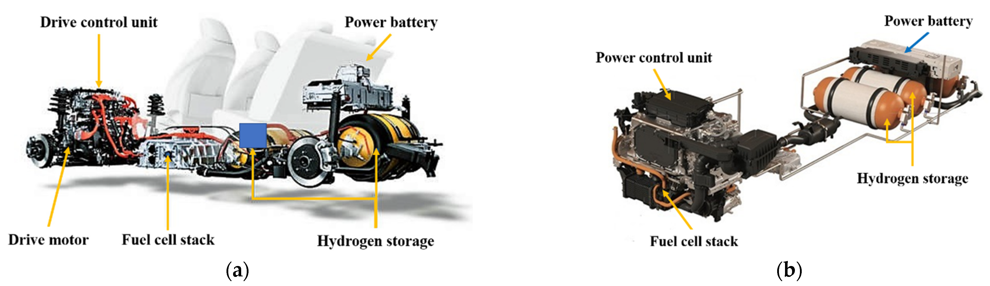
As the world’s first manufacturer to mass-produce FCEVs, test vehicle A was loaded with the first-generation fuel cells (with 114 kW power of electric reactor, 122.4 L hydrogen storage bottle capacity, 1.586 kWh power battery capacity, and 650 KM NEDC cycle) in 2014 and the second generation with higher performance in 2020 [
36,
37]. The power of the electric reactor is 128 kW, and it enables the second-generation test vehicle A to reach a range of 700 km on a 142.2 L hydrogen charge (World Light Vehicle Test Procedure, WLTP). Test vehicle B, to be released in 2019, has a system power of 95 kW and a power cell charge of 1.56 kWh, enabling a performance of 800 km (New European Driving Cycle, NEDC) with a range of 156.6 L of hydrogen. Hydrogen consumption per 100 km is an essential dimension in evaluating the performance of FCEVs, a reflection of the economic performance of the vehicle during operation, and one of the most critical technical priorities in the advancement of FCEV industrialization.
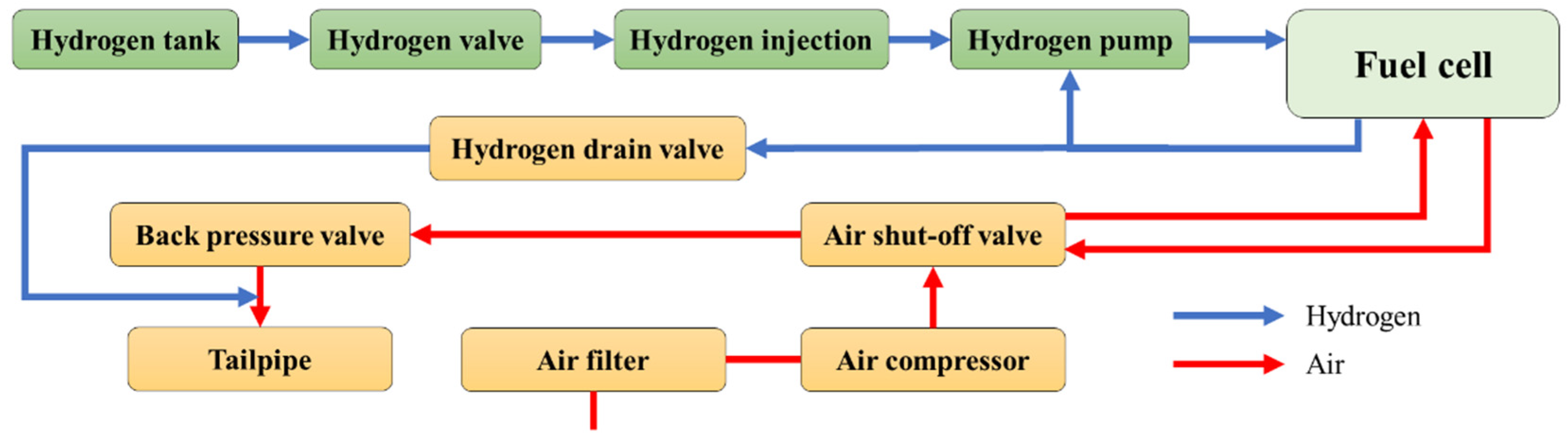
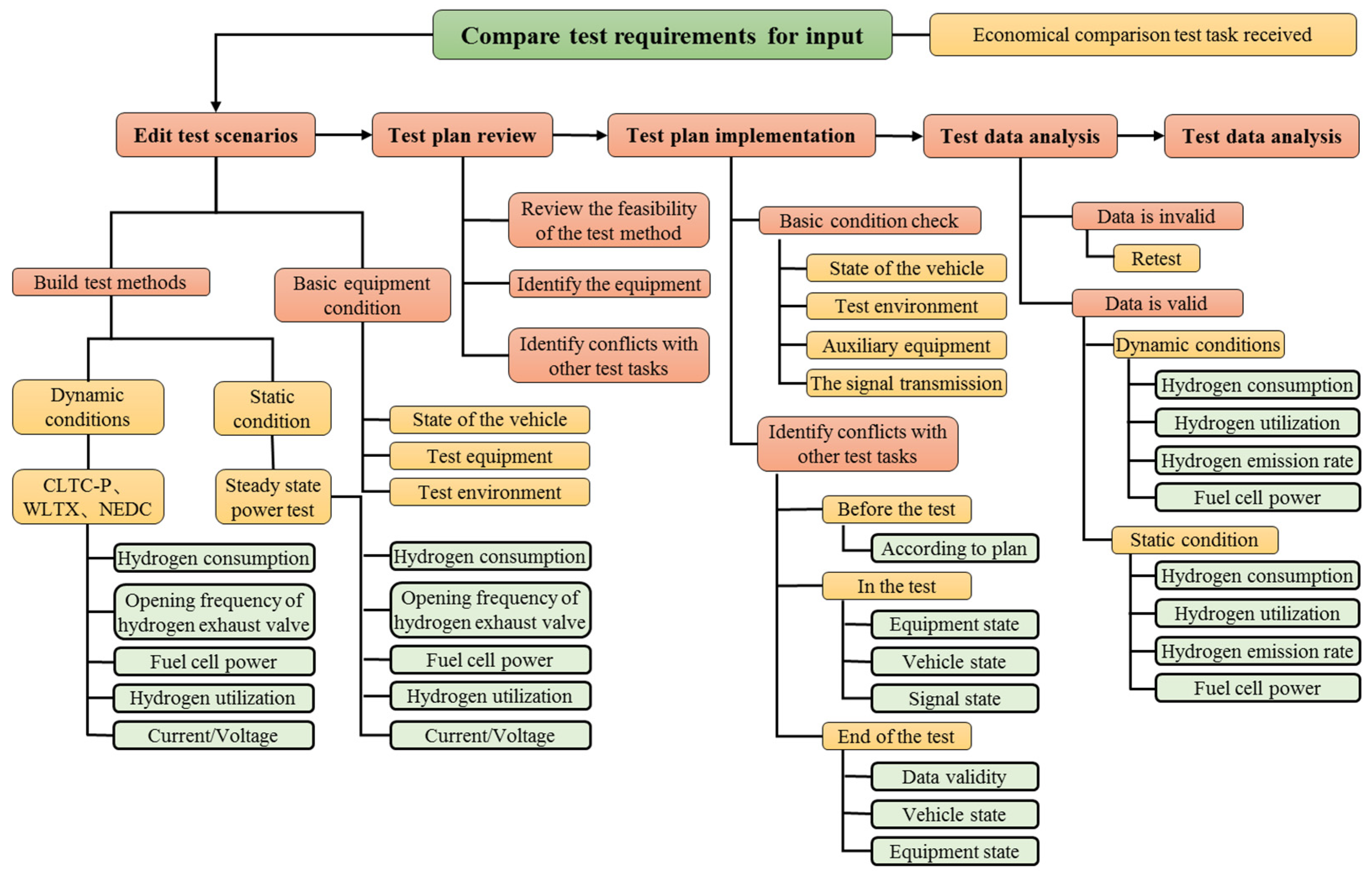
The hydrogen system piping arrangement at the fuel cell system level of the first-generation test vehicles A and B is analyzed in this study, particularly the hydrogen drain valve piping position. Additionally, it tests the Chinese Vehicle Driving Conditions-Passenger Car (CLTC-P) cycle, hydrogen consumption at different steady-state powers, and hydrogen emission rates from the FCS.
4. Results and Discussion
Referring to the test method of GB/T24554-2009 “Fuel Cell Engine Performance Test Method”, the output power was selected for both models and tested at 10 kW, 20 kW, 30 kW, 40 kW, 50 kW, 60 kW, 70 kW, and 80 kW, respectively. During the testing, the actual hydrogen flow consumption, the percentage of time the hydrogen discharge valve was open, and the change of hydrogen emission rate was observed at steady-state power. Since the steady-state power control of the fuel cell reactors fluctuates within a range, the actual output power of test vehicles A and B reactors is not strictly the set power at the operating point. So, to increase the comparability of the data, the hydrogen consumption per unit of energy is compared below.
Referring to the three hydrogen measurement methods given in GB/T35178-2017 “Fuel Cell Electric Vehicle Hydrogen Consumption Measurement Methods”, test vehicle A can use easier flow method to calculate the actual hydrogen consumption due to the bypass line installed in the fuel cell system. The value is measured by the mass flow meter installed in the supply line. The actual hydrogen consumption of the vehicle can only be calculated by using the temperature and pressure of the hydrogen storage tank before and after the test combined with the total volume of the high-pressure part of the onboard storage system due to the inconvenience of dismantling the bypass line of the vehicle. For test vehicle B, it should be noted that this method is different from GB/T35178-2017 “Fuel Cell Electric Vehicle Hydrogen Consumption Measurement Method”. It should be noted that this method is not strictly consistent with the external hydrogen storage tank required in the standard Pressure-Temperature Method.
4.1. Comparations of Hydrogen Consumption and Utilization under Steady-State Conditions
4.1.1. Comparative Analysis of Hydrogen Consumption
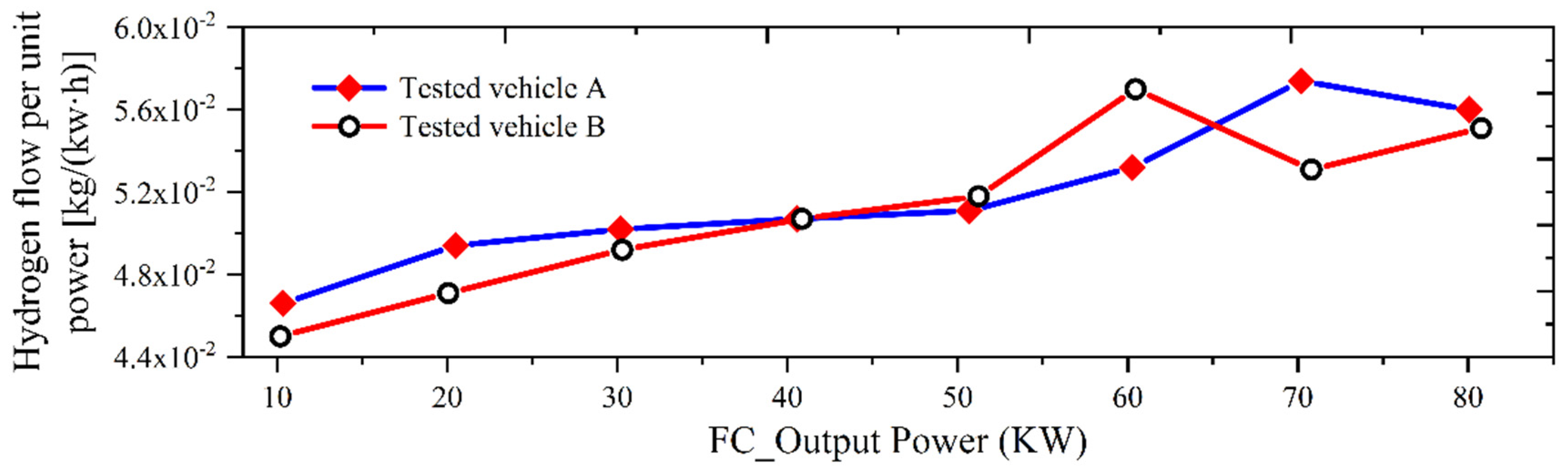
The actual hydrogen flow consumption of the fuel cell reactors of test vehicles A and B at different power steady-state conditions are shown in
Table 7. The hydrogen flow rate trend per unit power at steady-state power for test vehicles A and B are indicated in
Figure 8.
Figure 8 shows that the hydrogen consumption per unit power of test vehicle A is higher than that of test vehicle B when the reactor output is below 40 kW, higher than that of test vehicle A when the reactor output is between 40 kW and 60 kW, and higher than that of test vehicle B when the reactor output is between 70 kW and 80 kW. It is concluded that the fuel economy of test vehicle A is slightly lower than that of test vehicle B in steady-state at low power output (10 kW to 30 kW). The fuel economy of test vehicles A and B in steady-state operation at power output greater than 40 kW (50 kW to 80 kW) is better and worse.
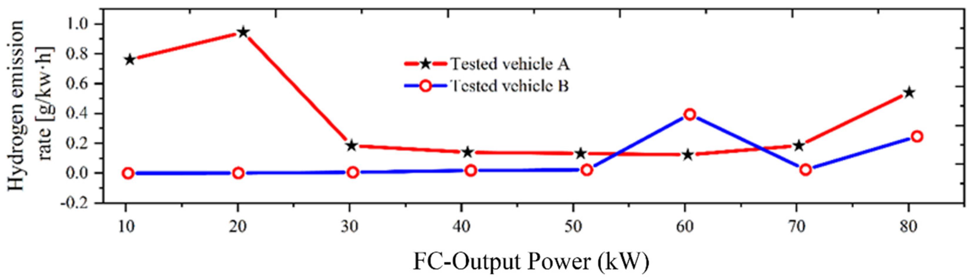
4.1.2. Comparison of Hydrogen Emission Rates at Steady-State Power
The actual hydrogen emission rates for the fuel cell reactors of test vehicles A and B models at different power steady-state operating conditions are compared in
Table 8. The trend of hydrogen emission rate per unit power for test vehicles A and B at steady-state power depending on different power is shown in
Figure 9.
It can be seen from
Figure 9 that the hydrogen emission rate of test vehicle B is better than that of test vehicle A at low power output (10 kW to 50 kW). At higher power output (60 kW to 80 kW), the hydrogen emission rate of test vehicle A is better than that of test vehicle B at 60 kW output. In contrast, at 70 kW and 80 kW output, the hydrogen emission rate of test vehicle B is better than that of test vehicle A. It can be concluded that the hydrogen emission rate of test vehicle B is better than that of test vehicle A at steady-state power conditions.
4.1.3. Subsubsection
The comparison of the actual hydrogen discharge valve opening time ratio between test vehicles A and B fuel cell reactors under different power steady-state operating conditions is shown in
Table 9.
The trend of the percentage of hydrogen discharge valve opening time per unit power for test vehicles A and B at steady-state power according to different power is shown in
Figure 10:
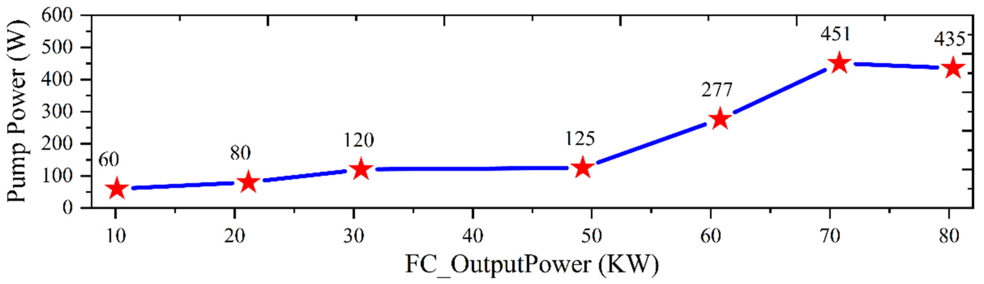
In terms of the opening timeshare of the hydrogen drain valve for steady-state power, the data on the opening timeshare of the hydrogen drain valve differs significantly between test vehicles A and B due to the difference in drain valve construction (vehicle A has an integrated drain function, while vehicle B only has a hydrogen drain function). The percentage of time that the hydrogen drain valve is open increases gradually with the output power of the reactor for both models. For test vehicle B, the rate of time that the hydrogen drain valve is available increases slowly when the output power of the reactor is less than 70 kW and increases rapidly when the output power of the reactor is greater than 70 kW. For test vehicle A, the percentage of time the hydrogen drain valve is open changes slowly when the output power is 10 kW and 20 kW and changes slowly when the output power is greater than 20 kW. After the power output is more significant than 20 kW, the percentage of time the hydrogen drain valve is open may be affected by the amount of water generated and proliferates.
4.2. Comparisons of Operating Characteristics under CLTC-P Cycle Conditions
The range of test vehicles A and B is based on the NEDC and WLTP conditions, respectively, and the content of test vehicle B is based on the NEDC conditions. The range of test vehicles A and B are tested for the first time in China under CLTC-P conditions. 13 CLTC-P cycle tests were carried out on the two models to fully accumulate test samples and observe more comprehensive test results. Consider that test car B cannot connect to the hydrogen flow measurement system on the laboratory test stand. The actual hydrogen emissions were calculated from the actual hydrogen consumption of the vehicle during each CLTC-P cycle and the theoretical hydrogen consumption measured by the mass flowmeter on the bypass line of test vehicle A and the actual hydrogen consumption of test vehicle B. The actual hydrogen emission was calculated by the temperature and pressure changes before and after the vehicle hydrogen storage bottle test combined with the volume of the hydrogen storage bottle. Theoretical hydrogen consumption is calculated according to the number of single cells in the stack and the instantaneous current of the stack. The actual hydrogen emission is obtained by subtracting the theoretical hydrogen consumption from the actual hydrogen consumption. The actual hydrogen emission rate is the ratio of the actual hydrogen emission to time.
4.2.1. Analysis of the Operating Characteristics of Test Vehicle A under Cyclic Conditions
The operating parameters of test vehicle A in 13 CLTC-P cycles are listed in
Table 10. In the 13 CLTC-P cycles, the distribution of mileage, actual hydrogen consumption, actual hydrogen consumption per unit mile, theoretical hydrogen consumption, theoretical hydrogen consumption per unit mile, hydrogen emission rate, and the percentage of hydrogen discharge valve opening time for each cycle are demonstrated.
For the 13 CLTC-P tests conducted by test vehicle A, the average driving range was 14.44 kM, the highest driving range was 14.6 kM (cycle 6), and the lowest driving range was 14.4 kM (cycle 7). The average actual hydrogen consumption was 141.093 g, the highest was 146.4 g (cycle 5), and the lowest was 134.8 g (cycle 8). In terms of actual hydrogen consumption per unit mile, the average hydrogen consumption per unit mile was 9.7723 g/kM, the highest value was 10.1667 g/kM (cycle 5), and the lowest value was 9.3611 g/kM (cycle 8). In terms of hydrogen emission rate, the average hydrogen emission rate was 1.556 g/(kW·h), the highest value of hydrogen emission rate was 1.988 g/(kW·h) (cycle 3), and the lowest value of hydrogen emission rate was 1.106 g/(kW·h) (cycle 2). Regarding the hydrogen vent opening time percentage, the average value of the hydrogen vent opening time percentage was 2.79%, the highest value was 3.11% (cycle 11), and the lowest value was 2.53% (cycle 6).
4.2.2. Analysis of Test Vehicle B Operating Characteristics under Cyclic Conditions
The mileage distribution, actual hydrogen consumption, actual hydrogen consumption per unit mile, theoretical hydrogen consumption, theoretical hydrogen consumption per unit mile, hydrogen emission rate, and the percentage of hydrogen discharge valve opening time for each of the 13 CLTC-P cycles are shown in
Table 11.
In the 13 CLTC-P tests conducted by test vehicle B, the authors used two methods to calculate hydrogen consumption per unit mile, theoretical hydrogen consumption, theoretical hydrogen consumption per unit mile, and hydrogen emission rate. The first method calculated the above parameters using the pressure and temperature at the beginning/ending of each cycle. The average value of actual hydrogen consumption was calculated as 119.0038 g. The average hydrogen consumption per unit mile was 8.2772 g/kM. The average hydrogen emission rate was 5.3967 g/kW·h, and the available hydrogen discharge valve percentage was 0.68%. In the second method, by recording the starting temperature and pressure of the first cycle of 13 CLTC-P cycles and the temperature and pressure at the end of the thirteenth cycle, the total mileage driven in 13 CLTC-P cycles was calculated as 186.9 kM, the total hydrogen consumption was 1476.6712 g, and the hydrogen consumption per unit mileage was 7.9009 g/kM. This is the total theoretical hydrogen consumption. The authors believe that the hydrogen consumption per unit mileage from the second calculation method is closer to the actual value, so the second algorithm is also used for the 100 km hydrogen consumption mentioned below.
4.2.3. Comparative Analysis of the Operating Characteristics of the Two Tested Vehicles
The test results show that vehicle A has a lower hydrogen emission rate while vehicle B has a lower hydrogen consumption rate. The actual hydrogen consumptions rates of vehicles A and B are 9.77 g/kM and 8.28 g/kM, respectively. The average hydrogen emission rates for vehicles A and B are 1.56 g/(kW·h) and 2.91 g/(kW·h) (since the error in the first method is too large, the conclusion of the second method is quoted), respectively, as shown in
Figure 11. Besides, the opening frequency of test vehicle A hydrogen drain valve is higher than that of test vehicle B, as the opening frequencies of the hydrogen drain valve for vehicle A and vehicle B are 2.79% and 0.68%, respectively.
The operating characteristics comparison of different vehicles is listed in
Table 12. FCEVs have fewer performance advantages but a more extended driving range than the current mainstream FCEVs and pure electric vehicles.
5. Conclusions
Through the analysis of hydrogen flow consumption at steady-state power, hydrogen flow consumption per unit power, hydrogen emission rate, and the percentage of time the hydrogen drain valve is open, the overall performance parameters of test vehicle B are better than those of test vehicle A. Test vehicle B’s hydrogen emission rate is higher than that of test vehicle A. However, test vehicle B’s hydrogen consumption per 100 km is still lower than that of test vehicle A, mainly due to the influence of the reactor performance, the hydrogen discharge valve opening strategy, and the performance of the brake energy recovery function.
Both test vehicles A and B consume similar amounts of hydrogen at the same steady-state power, with test vehicle B outperforming test vehicle A in terms of fuel economy in steady-state conditions at low power output (10 kW to 30 kW) and in steady-state conditions at power outputs more significant than 40 kW (50 kW to 80 kW). The hydrogen emission rate of test vehicle B is better than that of test vehicle A at steady-state power. In contrast, the actual hydrogen consumption of test vehicle B is approximately 7.90 g/km in the CLTC-P cycle and 9.77.23 g/km in test vehicle A, which is a significant difference.
In the 13 CLTC-P tests, the hydrogen consumption of vehicle B was erratic and jumped between individual cycles. In contrast, the hydrogen consumption of vehicle A was stable over a given cycle, with more minor variations between cycles. As vehicle A uses a hydrogen flow meter as the measurement method for hydrogen consumption, while vehicle B uses the temperature-pressure method for calculations, it can be concluded that the measurement method for hydrogen consumption has a significant influence on the experimental results. At the same time, the temperature-pressure method of the hydrogen consumption algorithm still has some shortcomings.


