
Nonlinear Vibration Analysis of Curved Piezoelectric-Layered Nanotube Resonator

Department of Mechanical and Industrial Engineering, University of Toronto, Toronto, ON M5S 3G8, Canada
Energies 2021, 14(23), 8031; https://doi.org/10.3390/en14238031
Submission received: 3 November 2021
/
Revised: 22 November 2021
/
Accepted: 22 November 2021
/
Published: 1 December 2021
(This article belongs to the Special Issue Novel Smart Materials and Structures for Energy Harvesting and Self-Powered Sensing)
Abstract
:Piezoelectric-based nano resonators are smart structures that can be used for mechanical sensors and actuators in miniature systems. In this study, the nonlinear vibration behavior of a curved piezoelectric-layered nanotube resonator was investigated. The curved structure comprises a core nanotube and a slender layer of piezoelectric material covering the inner nanotube where a harmonic voltage is applied to the piezoelectric layer. Applying the energy method and Hamiltonian principle in association with non-local theories, the governing equations of motion of the targeted system are obtained. Then, the problem is solved using the Galerkin and multiple scales methods, and the system responses under external excitation and parametric load are found. Various resonance conditions are investigated including primary and parametric resonances, and the frequency responses are obtained considering steady state motions. The effects of different parameters such as applied voltage, piezoelectric thickness, and structural curvature on the system responses are investigated. It is shown that the applied harmonic voltage to the piezoelectric layer can cause a parametric resonance in the structural vibration, and the applied harmonic point load to the structure can cause a primary resonance in the vibration response. Considering two structural curvatures including quadratic and cubic curves, it is also found that the waviness and curve shape parameters can tune the nonlinear hardening and softening behaviors of the system and at specific curve shapes, the vibration response of the targeted structure acts similar to that of a linear system. This study can be targeted toward the design of curved piezoelectric nano-resonators in small-scale sensing and actuation systems.
1. Introduction
Nano resonators are emerging materials and structures to be used for sensing and actuation in microelectromechanical (MEMS) and nanoelectromechanical systems (NEMS). The role of nanotubes can be widely observed in the baseline of nano resonators due to their brilliant properties since their discovery in recent decades [1,2]. One of the main aspects of nanotube behaviors for mechanical sensing and actuation is their vibrational response, and therefore the research of nanotubes vibrations has been observed in various studies using different methods, such as experimental methods, molecular dynamics, and continuum mechanic theories [3,4,5,6]. Although the two first methods are more costly and time consuming, continuum theories are more convenient in modeling the dynamics of aforementioned structures [6]. However, the classical continuum theories are not fully reliable due to the effects of small sizes [6]. This is because, at scales of small lengths, the material’s microstructure, including the lattice formation of atomic configuration and internal atomic forces, play an important role and consequently, the discrete microstructure cannot be standardized as a continuum model [6]. Thus, non-classical theories have been recently developed and utilized for understanding the behavior of nano-sized systems [6]. One of the important non-classical theories is Eringen’s non-local theory, which briefly indicates that the stress at a reference point is dependent on the strain field at every point in the body [7,8,9]. Thus, the stress tensor at a specific point is the function of strain tensors at all points, whereas in classical models the stress and strain tensors are uniquely dependent on each other at the same point [9]. The non-local theory considers a range of internal microstructure forces in the constitutive equations, which can potentially be used for modeling nano systems. Therefore, this theory has extensively been used in studying various nano structures [9,10,11,12,13].
By comparison, a piezoelectric material basically refers to a type of solid state material that shows a coupling between its electrical, mechanical, and thermal states by applying mechanical stress to dielectric crystals [14]. It was revealed that when an electric field is applied to these materials, mechanical stress or strain are generated in their structures and, furthermore, applying mechanical stress leads to electric charge generation through the structure [14]. The outstanding properties of piezoelectric materials and their significant application in small scale electromechanical structures have attracted scientists to investigate the dynamics and vibrational behaviors of piezoelectric-based nanostructures [15,16,17]. For example, the vibrational behavior of zinc oxide-carbon nanotubes as pressure stress sensors was studied by Wang and Chew [18]. These structures were fabricated by coating the piezoelectric material on the nanotube and linear assumptions were developed for modeling the corresponding vibration [18]. In this respect, the vibration of piezoelectric-layered nano beams, non-local instability behavior of piezoelectric-layer nanotubes, and the vibration of piezoelectric-based nano plates have been studied recently [19,20,21].
In the design of nanotube-based resonators, the structure may possess a curvature of its shape which can be due to the natural geometrical properties or may be intentionally formed to obtain specific mechanical properties for the system. This curvature can play a critical role in the system’s mechanical behavior. Thus, investigating the effect of structural curvature on the nanotube mechanical behavior has been a fascinating research direction in recent years. In one of the pioneer works, Berhan et al. investigated the effects of the non-straight shapes on the mechanical properties of nano structures [22]. Their modeling showed that the Young’s moduli in nanotube ropes is directly dependent on the waviness of these structures [22]. Zare et al. incorporated non-local strain gradient theory to study the vibrations of shell-like nanotubes with structural curvature [23]. Plastic buckling of curved nanotubes was also investigated by Malekian, where the static stability response of curved carbon nanotubes under elastoplastic behavior was studied [24]. In another paper, the dynamic characteristics of a curved fluid-conveying nanotube considering the size-dependency were investigated [25]. The vibration analysis of functionally graded porous curved nanotubes was carried out using strain gradient theory [26]. In another study, a unified approach was developed to model the vibration of curved nanotubes by means of the Non-Uniform Rational B-Spline method (NURBS) [27].
In this study, the vibration behavior of a curved piezoelectric-layered nanotube was modeled and solved. Applying the energy method, the Lagrangian formula, and the Hamiltonian principle associated with non-local theories, the governing equation of motion of the corresponding system was determined. In the next step, the problem was solved using the Galerkin and multiple scales methods, and the system responses under external excitation and parametric load were found [28]. The piezoelectric layer is taken to be slender and the applied voltage is a harmonic function of time. Two cases of resonance condition were evaluated, known as primary and parametric resonances, and the frequency responses were obtained for steady state motion for each case. The effects of different parameters, such as applied voltage, piezoelectric thickness, and the shape of the structure’s curvature on the system responses, were investigated. For the last item, two typical types of curves, namely, quadratic and cubic shapes, were considered for the structure, and the influence of changing the shape on the frequency–amplitude responses are plotted and discussed. Overall, this study is useful for the design and analysis of piezoelectric-based nano resonators with structural curvature, for application to mechanical sensing and actuation systems in the small scale.
2. Mathematical Modeling
Figure 1 schematically represents a piezoelectric-layered nanotube with a general two-dimensional curvature along the structure under a general external force .
The outer layer shown in dark is the piezoelectric layer surrounding the inner nanotube. For modeling the dynamic behavior of the system, one can consider the use of the Euler–Bernoulli beam theory in which the displacement fields and corresponding strain are written in the following general form [29]:
where and indicate the transverse and longitudinal displacements, respectively. refers to the deflection of the beam model centroid axis along the system as a function of the horizontal axis x. In addition, the constitutive equations for the slender piezoelectric layer along the beam-type model is written as the following reduced form [30]:
Where and are the respective von Karman stress and the strain along the structure. indicates the electric field in the axial direction such that and is the electric potential [30]. shows the electrical displacement in axial direction. Additionally, the constants , and refer to the linear elastic constant of piezoelectric, piezoelectric constant, and the dielectric constant, respectively [30]. It should be noted that due to the symmetry and slenderness of the beam-type model of piezoelectric layer, the electrical effects on the other directions do not exist in the corresponding constitutive equations. In addition, the following relationships hold for the strains, bending moments, and shear forces of each layer:
where and correspond to the outer piezoelectric layer and the inner nanotube, respectively. In addition, , , and indicate the cross-section area, bending moment, and shear force along the beam, respectively. The energy method and Hamiltonian principle are used here to obtain the governing equation of motion of the system. Thus, the equations of strain energy, kinetic energy, and external force work should be carried out. Accordingly, the strain energy of the proposed system is presented by the following formulation:
Substituting Equations (3)–(5) into the above equation gives:
The kinetic energy and the external force work are respectively written as:
To obtain the governing equation, the Lagrangian function of the system is written as:
Such that T, U and W denote the total kinetic energy, potential energy, and the external force work, respectively. By means of the Variational approach, the variation in the Lagrangian function in a period of time would be zero, and consequently one can set:
Thus, using the boundary conditions’ properties and setting the coefficients of the variations equal to zero, one can obtain:
To add the influence of the nano size effect, the non-local theory is applied to the bending moment of the system. Hence, the following equation is taken for the structure bending moment according to Eringen’s theory [9]:
In which E and I show the modulus of elasticity and cross-sectional moment of inertia for the nanotube, respectively, and denotes the nonlocal parameter originated from the small scale size of the nano structure. Applying the above equation to Equation (12), the governing equations of motion for the vibration of the structure are:
Additionally, the relationship between transversal and longitudinal displacement for the system with curvature with immovable ends is approximated as [27]:
In order to facilitate the solution procedure, the following dimensionless parameters are defined and, consequently, the obtained results are determined in the dimensionless form:
where is the harmonic voltage amplitude and is the dimensionless structure curvature.
3. Solution Procedures
In this section, the Galerkin method is utilized for simplifying the obtained equation of motion from the previous section [28]. The discretized form of transversal vibration for the fundamental mode has been considered here. The applied voltage is taken to be a harmonic function of time with the frequency , and an external load of is considered to be as a harmonic point load with the amplitude of and frequency of imposed at an arbitrary distancealong the structure as:
After applying the Galerkin method and the concept of normal modes’ orthogonality, the ordinary differential equation of the system’s first mode time response is obtained as:
where the linear frequency , and the constant coefficients and in the above equation are presented in Appendix A, based on the physical and geometrical properties of the curved structure. The multiple scales method is now employed for solving the nonlinear differential equation presented Equation (20) [28]. For this purpose, a small damping term µ is added to the equation, and in order to insert the effect of nonlinear terms and external forces, the corresponding coefficients should be properly ordered by inserting a small dimensionless perturbation parameter known as ε [28]. Accordingly, the equation is rewritten as:
According to the basic idea of the multiple scales method, the following time scales are introduced [28]:
where the independent variable indicates the time scale [28]. Therefore, the derivatives with respect to are the expansions in terms of the partial derivatives with respect to as [28]:
where . The considered solution of Equation (21) can be written as the following expansion form [28]:
Then, the solution can be approximated up to the second order of the above expression requiring and only [28]. Thus, by substituting Equations (23) and (24) into Equation (21), and equating the terms with the same power of ε, gives:
The general solution of Equation (25) can be obtained as:
where is an unknown complex function and is the complex conjugate of [28]. Substituting Equation (28) into (26), one obtains:
where CC is the complex conjugate of the terms. The elimination of secular terms from the above equation requires:
which means that the amplitude is independent from or . Then, the solution of Equation (29) considering both private and homogenous solutions is equal to:
Now Equations (28) and (31) are substituted into Equation (27) which, after some mathematical simplification and considering the elimination of the terms correspond to , leads to:
where the superscript prime in Equation (32) indicates the derivative with respect to . From the above equation, it can be seen that three different resonances may occur in the system, including two primary resonances when or , and one parametric resonance when . In addition, simultaneous resonances may be seen when or . Here, two important resonances are investigated for the proposed model in the following sections.
3.1. Case A:
This case investigates a parametric resonance condition caused by the external harmonic voltage applied to the piezoelectric layer. Note that a detuning parameter is introduced to quantitatively describe the nearness of the applied voltage frequency to the natural frequency of the system , as presented by [28]. Considering such a parametric resonance condition due to the harmonic applied voltage, and eliminating the secular terms from Equation (32), gives:
In solving the above differential equation, one can write in a polar form where the amplitude and the phase are real functions of [28]. Applying the polar form in the above equation and separating the real and imaginary parts gives:
Where . For the steady-state motion of the parametric resonance, one should set [28]. Thus:
Solving the above system gives the relationship between the amplitude of vibration and the detuning parameter , i.e., the nearness of the external voltage frequency to in this parametric resonance case. Accordingly, the parameter defines the relationship between the applied voltage frequency and the amplitude of vibration. Such a relationship, which is known as the frequency–amplitude relationship of the steady-state motion, is obtained as:
The above equation shows the frequency response of the structure for the considered resonance case. In addition, the conditions of having solutions for Equation (36) can be easily obtained by setting the terms under square roots to be greater than zero. According to the above equation, it can be found that the first condition required to obtain a solution is when . Additionally, positive requires , and when is negative, is required to obtain a solution.
3.2. Case B:
This case is a primary resonance condition that occurs due to the external harmonic point load applied to the structure. In this case, the detuning parameter is also defined to quantitatively express the nearness of the external excitation frequency to the linear natural frequency of the system as . For this primary resonance, the elimination of secular terms from Equation (32) leads to:
Using a similar procedure to the previous case when using the polar form , the frequency–amplitude relationship of the steady state motion is obtained as [28]:
The above equation shows the relationship between the amplitude of vibration and the detuning parameter , i.e., the nearness of the external force frequency to the natural frequency in this primary resonance case. In fact, the value of relates the amplitude of vibration to the frequency of the external load. As seen, the effects of all nonlinear terms appear on the response relationships of this case, and the condition for the existence of solution is , where the peak value of amplitude is obtained from Equation (38). The first approximate solution also becomes:
Where , and shows the higher order terms.
4. Results and Discussion
In this section, the vibration behavior of the targeted curved nano structure is analyzed by computing the obtained solution relationships using numerical values. For this purpose, the physical and geometrical properties of the carbon nanotube structure and ZnO piezoelectric layer were selected based on the references [27,30]. As the model considers a general form of planar curvature, two types of curvature, namely, quadratic and cubic, are examined for this purpose. Accordingly, the frequency–amplitude responses under the external and parametric resonances are studied for both curves, and the effects of the piezoelectric layer and the shape waviness are investigated in the results. Figure 2 represents the considered quadratic curves of the piezoelectric layer nanotube studied in the previous section. As shown, different degrees of waviness are considered for this case. It should be noted that the waviness parameter r indicates the ratio between the vertical position of the nanotube middle point and the horizontal distance of the two ends. Thus, the influence of changing r is investigated as an important parameter of the structure’s quadratic shape. Additionally, different formations of cubic curves are represented in Figure 3. In order to study and compare different types of this curve type, the maximum vertical position of the structure is kept constant and the horizontal position of this peak point , is varied from the left end to the middle, and the effect of this variation is taken into the account for the results. The detailed mathematical expressions of the considered curvatures and the descriptions of the quadratic waviness parameter r and the cubic curve shape parameter are presented in Appendix B.
The responses of the structure under parametric resonance are represented in Figure 4, Figure 5 and Figure 6 for the aforementioned quadratic and cubic curves. A typical frequency–amplitude response of the structure under parametric resonance is depicted in Figure 4a, such that the dashed line indicates the unstable solution which does not occur in the physical behavior of the system [28]. The jump phenomena may occur in the system when the voltage frequency approaches the natural frequency from the right side by decreasing the detuning parameter and, accordingly, a sudden shift occurs in the amplitude of vibration to the upper curve, following the arrows [28]. Figure 4b is known as the response curve and depicts the influence of varying amplitude of parametric excitation on the vibration amplitude, which can be assessed by changing the amplitude of the applied harmonic voltage. The dashed line denotes the unstable solution and again, the jump phenomenon is observed by the red arrows depending on increasing or decreasing the excitation amplitude [28].
The frequency responses of the quadratic curve with different waviness are shown in Figure 5a. Accordingly, for the lower waviness, the hardening behavior is observed and by increasing this parameter, the system response moves to the left, at which the system becomes softer. The system response for a special quadratic curvature is also shown in Figure 4, which is called the critical quadratic curvature. As is obvious, no nonlinearity is observed for the parametric resonance in the critical quadratic curvature. The response curve, which is the variation of the vibration amplitude with respect to changing the parametric excitation amplitude, is represented in Figure 5b for different degrees of quadratic curve waviness. Note that the amplitude of parametric excitation can be varied by changing the harmonic applied voltage. Additionally, it is obvious that the increase in the waviness reduces the amplitude of vibration and the jump in the system.
The frequency response of the structure with a cubic curve due to parametric resonance is depicted in Figure 6a, and the effect of peak point position is studied here. It is clear that when the position is at the very end, the system is extremely hard, whereas when the position approaches the middle, the system shows a softening response. It should be noted that for the critical cubic curvature, i.e., around , the linear behavior of the system is represented by dashed purple lines. The response curve of the cubic curvature and the effect of the maximum point position is represented in Figure 6b. Accordingly, the more the peak point moves toward the middle, the lower the amplitude of vibration and jump occur in the system. Thus, this peak position can be taken as an important parameter to understand the vibration behavior, and can be used to find the required response in terms of vibration amplitude, hardening–softening, and even linear behavior for the structure with a cubic curvature.
The frequency responses of the curved system under primary resonance are represented in Figure 7 and Figure 8 for both aforementioned curvatures. The effect of quadratic curve waviness on the hardening–softening behavior of the quadratic curve structure is seen in Figure 7a. Accordingly, for small waviness, the system behavior is extremely hard, whereas by increasing the waviness the system tends to be close to the linear behavior, and then bends to the left side, which results in softening behavior. This shift also reduces the structure’s amplitude of vibration. Thus, the curve waviness can be considered as a control parameter in order to find the desirable behavior whether it is soft, hard, or even linear for such a nonlinear nano system. As shown by the dashed red curves in Figure 7a, for the critical structure curvature , the frequency–amplitude relationship is linear, which as an important finding of this study. As a typical parameter study, the effect of piezoelectric layer thickness on the frequency response is shown in Figure 7b in which for a higher thickness, the amplitude of vibration considerably decreases.
The effect of the peak point position on the frequency response of the structure with cubic curvature is investigated in Figure 8a for the primary resonance. When the position of this point is close to the structure’s end, the system’s nonlinear behavior is hard. As the position moves toward the middle, not only does softening behavior appears, but the vibration amplitude also decreases, which is an interesting result to be used in the prediction and also the design of such a curved system. In Figure 8b, the piezoelectric thickness effect is analyzed when the maximum point position is close to the end or to the middle. For both hard and soft behaviors caused by the peak point position, the thickness growth lowers the amplitude, and the amplitude is smaller for the softening behavior in comparison with the harder one. Again, for the frequency response of the critical curvature in which , the system shows a linear vibration in spite of the presence of nonlinear terms in the general equation, which is a very important finding.
5. Conclusions
Nonlinear vibrations of a piezoelectric-layered nanotube under an applied harmonic voltage were studied in this work. The governing equations of motion were developed by means of the energy method and non-local theory considering the effect of structure curvature. The Galerkin approach and the multiple scales method were then employed to solve the equations. The vibration responses and frequency–amplitude relationships were obtained analytically for two important resonance cases, namely, primary and parametric resonances. The effects of physical and geometrical parameters on the vibration behavior and frequency responses of the proposed system were studied. Two important curvatures, namely, quadratic and cubic shapes, were investigated for the structure, and the influences of the corresponding curves on the nonlinear behavior of the system were studied. It was shown that the hardening, softening, and linear behaviors of the system could be achieved depending on the waviness of the structure’s curve. This study can be utilized for the analysis of curved nanostructures comprising piezoelectric layers to identify the desirable linear or nonlinear behaviors, for the design of micro/nano scale smart sensors and actuators.
Funding
This research received no external funding.
Institutional Review Board Statement
Not applicable.
Informed Consent Statement
Not applicable.
Data Availability Statement
The data presented in this study are available on request from the corresponding author.
Acknowledgments
The author would like to appreciate Ebrahim Esmailzadeh for his help and advice in preparing this manuscript.
Conflicts of Interest
The author declares no conflict of interest.
Appendix A
The linear natural frequency and the constant coefficients of Equation (20) are found as:
Appendix B
The mathematical expression for the quadratic curves of Figure 2 can be written as:
where is the vertical position of the nanotube middle point, and indicates the horizontal distance of the two ends of the structure. The quadratic waviness has been defined as the ratio between the vertical position of nanotube middle point and the horizontal distance of the two ends or . Knowing that, for the dimensionless model developed here, , the equation of the quadratic curves in terms of can be simplified as:
Additionally, the mathematical expression for the cubic curves shown in Figure 3 can be given in the following dimensionless form:
The maximum vertical position of the structure was considered to be a constant which is located at an arbitrary horizontal position of defined as the cubic curve shape parameter. At this point, the slope of the curve is also zero, as shown in Figure 3. Note that the vertical position of the curve is also zero at the two ends of the structure. Therefore, the unknown coefficients of the above equation , can be easily calculated by solving the following system of linear algebraic equations for a given :
References
- Coleman, J.N.; Khan, U.; Blau, W.J.; Gun’ko, Y.K. Small but strong: A review of the mechanical properties of carbon nanotube–polymer composites. Carbon 2006, 44, 1624–1652. [Google Scholar] [CrossRef]
- Baughman, R.H.; Zakhidov, A.A.; De Heer, W.A. Carbon nanotubes--the route toward applications. Science 2002, 297, 787–792. [Google Scholar] [CrossRef] [PubMed] [Green Version]
- Abadal, G.; Davis, Z.J.; Borrisé, X.; Hansen, O.; Boisen, A.; Barniol, N.; Pérez-Murano, F.; Serra, F. Atomic force microscope characterization of a resonating nanocantilever. Ultramicroscopy 2003, 97, 127–133. [Google Scholar] [CrossRef]
- Kim, J.; Park, S.; Park, J.; Lee, J. Molecular dynamics simulation of elastic properties of silicon nanocantilevers. Nanoscale Microscale Thermophys. Eng. 2006, 10, 55–65. [Google Scholar] [CrossRef]
- Roudbari, M.A.; Jorshari, T.D.; Lü, C.; Ansari, R.; Kouzani, A.Z.; Amabili, M. A review of size-dependent continuum mechanics models for micro-and nano-structures. Thin-Walled Struct. 2022, 170, 108562. [Google Scholar] [CrossRef]
- Sudak, L. Column buckling of multiwalled carbon nanotubes using nonlocal continuum mechanics. J. Appl. Phys. 2003, 94, 7281–7287. [Google Scholar] [CrossRef]
- Eringen, A.C. Nonlocal Polar Field Models; Academic: New York, NY USA, 1976. [Google Scholar]
- Eringen, A.C.; Edelen, D. On nonlocal elasticity. Int. J. Eng. Sci. 1972, 10, 233–248. [Google Scholar] [CrossRef]
- Eringen, A.C. On differential equations of nonlocal elasticity and solutions of screw dislocation and surface waves. J. Appl. Phys. 1983, 54, 4703–4710. [Google Scholar] [CrossRef]
- Evgrafov, A.; Bellido, J.C. From non-local Eringen’s model to fractional elasticity. Math. Mech. Solids 2019, 24, 1935–1953. [Google Scholar] [CrossRef] [Green Version]
- Gonçalves, E.H.; Ribeiro, P. Modes of vibration of single- and double-walled CNTs with an attached mass by a non-local shell model. J. Vib. Eng. Technol. 2021, 1–9. Available online: https://link.springer.com/article/10.1007%2Fs42417-021-00381-z (accessed on 2 November 2021). [CrossRef]
- Vantadori, S.; Luciano, R.; Scorza, D.; Darban, H. Fracture analysis of nanobeams based on the stress-driven non-local theory of elasticity. Mech. Adv. Mater. Struct. 2020, 1–10. Available online: https://www.tandfonline.com/doi/full/10.1080/15376494.2020.1846231 (accessed on 2 November 2021). [CrossRef]
- Babaei, A. Forced vibration analysis of non-local strain gradient rod subjected to harmonic excitations. Microsyst. Technol. 2021, 27, 821–831. [Google Scholar] [CrossRef]
- Jalili, N. Piezoelectric-Based Vibration Control: From Macro to Micro/Nano Scale Systems; Springer Science and Business Media: Boston, MA, USA, 2009. [Google Scholar]
- Ke, L.L.; Wang, Y.S.; Wang, Z.D. Nonlinear vibration of the piezoelectric nanobeams based on the nonlocal theory. Compos. Struct. 2012, 94, 2038–2047. [Google Scholar] [CrossRef]
- Yan, Z.; Jiang, L. The vibrational and buckling behaviors of piezoelectric nanobeams with surface effects. Nanotechnology 2011, 22, 245703. [Google Scholar] [CrossRef] [PubMed]
- Ke, L.L.; Wang, Y.S. Thermoelectric-mechanical vibration of piezoelectric nanobeams based on the nonlocal theory. Smart Mater. Struct. 2012, 21, 025018. [Google Scholar] [CrossRef]
- Wang, C.; Li, L.; Chew, Z. Vibrating ZnO–CNT nanotubes as pressure/stress sensors. Physica E Low Dimens. Syst. Nanostruct. 2011, 43, 1288–1293. [Google Scholar] [CrossRef]
- Nazemizadeh, M.; Bakhtiari-Nejad, F.; Assadi, A. Nonlinear vibration of piezoelectric laminated nanobeams at higher modes based on nonlocal piezoelectric theory. Acta Mech. 2020, 231, 4259–4274. [Google Scholar] [CrossRef]
- Hosseini, M.; Bahaadini, R.; Jamali, B. Nonlocal instability of cantilever piezoelectric carbon nanotubes by considering surface effects subjected to axial flow. J. Vib. Control 2018, 24, 1809–1825. [Google Scholar] [CrossRef]
- Ebrahimi, F.; Hosseini, S.H.S. Nonlinear dynamic modeling of smart graphene/piezoelectric composite nanoplates subjected to dual frequency excitation. Eng. Res. Express 2020, 2, 025019. [Google Scholar] [CrossRef]
- Berhan, L.; Yi, Y.; Sastry, A. Effect of nanorope waviness on the effective moduli of nanotube sheets. J. Appl. Phys. 2004, 95, 5027–5034. [Google Scholar] [CrossRef] [Green Version]
- Zare, J.; Shateri, A.; Beni, Y.T.; Ahmadi, A. Vibration analysis of shell-like curved carbon nanotubes using nonlocal strain gradient theory. Math. Methods Appl. Sci. 2020. Available online: https://onlinelibrary.wiley.com/doi/10.1002/mma.6599 (accessed on 2 November 2021). [CrossRef]
- Malikan, M. On the plastic buckling of curved carbon nanotubes. Theor. Appl. Mech. Lett. 2020, 10, 46–56. [Google Scholar] [CrossRef]
- Dini, A.; Hosseini, M.; Nematollahi, M.A. On the size-dependent dynamics of curved single-walled carbon nanotubes conveying fluid based on nonlocal theory. Acta Mech. 2021, 1–17. Available online: https://link.springer.com/article/10.1007%2Fs00707-021-03081-7 (accessed on 2 November 2021). [CrossRef]
- Babaei, H. Nonlinear analysis of size-dependent frequencies in porous FG curved nanotubes based on nonlocal strain gradient theory. Eng. Comput. 2021, 1–18. Available online: https://link.springer.com/article/10.1007%2Fs00366-021-01317-7 (accessed on 2 November 2021). [CrossRef]
- Askari, H. Nonlinear vibration and chaotic motion of uniform and non-uniform carbon nanotube resonators. Master’s Thesis, University of Ontario Institute of Technology, Oshawa, ON, Canada, 2014. [Google Scholar]
- Nayfeh, A.H.; Mook, D.T. Nonlinear Oscillations; Wiley VCH: Weinheim, Germany, 2008. [Google Scholar]
- Reddy, J.; Singh, I. Large deflections and large-amplitude free vibrations of straight and curved beams. Int. J. Numer. Methods Eng. 1981, 17, 829–852. [Google Scholar] [CrossRef]
- Zhang, J.; Wang, R.; Wang, C. Piezoelectric ZnO-CNT nanotubes under axial strain and electrical voltage. Physica E Low Dimens. Syst. Nanostruct. 2012, 46, 105–112. [Google Scholar] [CrossRef]
Figure 1.
Schematic model of the curved nanotube with slender piezoelectric layer.

Figure 2.
The quadratic curve with different waviness considered for the structure.

Figure 3.
The effect of the cubic curve shape parameter on the structural curvature.
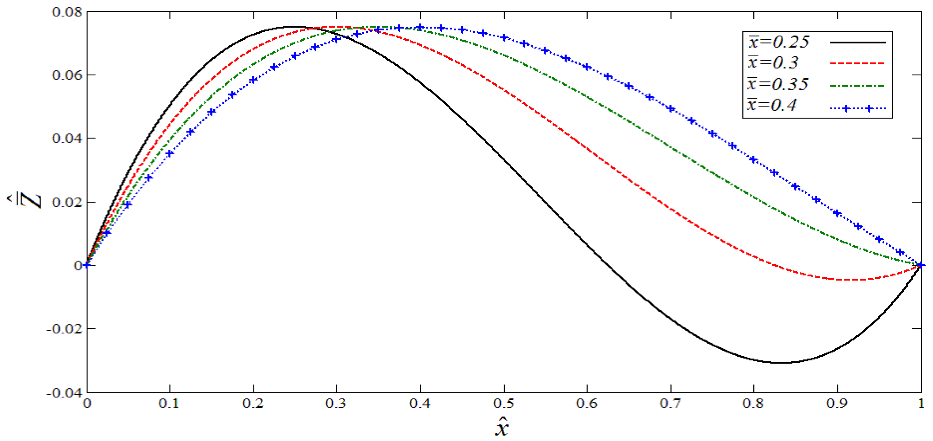
Figure 4.
(a) A typical frequency–amplitude response of the system for the parametric resonance; (b) a typical response curve of the system for the parametric resonance.
Figure 4.
(a) A typical frequency–amplitude response of the system for the parametric resonance; (b) a typical response curve of the system for the parametric resonance.

Figure 5.
(a) Quadratic curvature waviness effect on the frequency response in the parametric resonance; (b) quadratic curvature waviness effect on the response curve in the parametric resonance.
Figure 5.
(a) Quadratic curvature waviness effect on the frequency response in the parametric resonance; (b) quadratic curvature waviness effect on the response curve in the parametric resonance.

Figure 6.
(a) Cubic curvature shape effect on the frequency response of the parametric resonance; (b) cubic curvature shape effect on the response curve of the parametric resonance.
Figure 6.
(a) Cubic curvature shape effect on the frequency response of the parametric resonance; (b) cubic curvature shape effect on the response curve of the parametric resonance.

Figure 7.
(a) Quadratic curvature waviness effect on the response of the primary resonance; (b) piezoelectric thickness effect on the response of the quadratic curve primary resonance.
Figure 7.
(a) Quadratic curvature waviness effect on the response of the primary resonance; (b) piezoelectric thickness effect on the response of the quadratic curve primary resonance.

Figure 8.
(a) Cubic curve shape effect on the frequency response of the primary resonance; (b) piezoelectric thickness effect on the response of the cubic curve primary resonance.
Figure 8.
(a) Cubic curve shape effect on the frequency response of the primary resonance; (b) piezoelectric thickness effect on the response of the cubic curve primary resonance.

Publisher’s Note: MDPI stays neutral with regard to jurisdictional claims in published maps and institutional affiliations. |
© 2021 by the author. Licensee MDPI, Basel, Switzerland. This article is an open access article distributed under the terms and conditions of the Creative Commons Attribution (CC BY) license (https://creativecommons.org/licenses/by/4.0/).
Share and Cite
MDPI and ACS Style
Saadatnia, Z. Nonlinear Vibration Analysis of Curved Piezoelectric-Layered Nanotube Resonator. Energies 2021, 14, 8031. https://doi.org/10.3390/en14238031
AMA Style
Saadatnia Z. Nonlinear Vibration Analysis of Curved Piezoelectric-Layered Nanotube Resonator. Energies. 2021; 14(23):8031. https://doi.org/10.3390/en14238031
Chicago/Turabian StyleSaadatnia, Zia. 2021. "Nonlinear Vibration Analysis of Curved Piezoelectric-Layered Nanotube Resonator" Energies 14, no. 23: 8031. https://doi.org/10.3390/en14238031
Note that from the first issue of 2016, this journal uses article numbers instead of page numbers. See further details here.